Асимптоты графика функции
Часто задание на нахождение асимптот функции встречается в курсе математического анализа, в частности при решении задач на тему исследования функции. Для того, чтобы успешно ответить на вопрос: как найти асимптоты функции? необходимо уметь вычислять пределы, понимать что они собой представляют, знать основные методы решения пределов. Если всё это вы умеете на должном уровне, тогда найти асимптоты для вас не будет проблемой. Итак, что такое асимптота? Асимптота это линия, к которой бесконечно приближается ветвь графика функции. Чтобы было наглядно, посмотрите на изображения представленные ниже.
Обратите внимание, что соприкосновения между асимптотой и графиками нет, и не должно быть. Асимптота бесконечно приближается к графику функции. Давайте рассмотрим какие виды асимптоты функции бывают и как их находить, но о последнем будет рассказано далее.
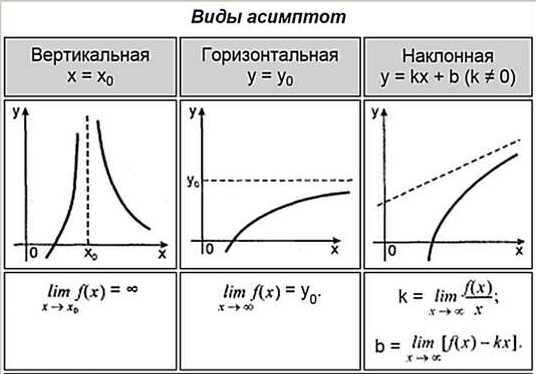
Из таблицы узнаем, что асимптоты у функции бывают трех видов: вертикальные, горизонтальные, наклонные. Каждую найти асимптоту функции нужно по своему. Для этого нужны лимиты. Сколько бывает асимптот всего у функции? Ответ: ни одной, одна, две, три… и бесконечно много. У каждой функции по разному.
Вертикальные асимптоты
Чтобы найти данный вид асимптот необходимо найти область определения заданной функции и отметить точки разрыва. В этих точках предел функции будет равен бесконечности, а это значит, что функция в этой точке бесконечно приближается к линии асимптоты.
Горизонтальные асимптоты
Необходимо устремить аргумент лимита функции к бесконечности. Если предел существует и равен числу, то горизонтальная асимптота будет найдена и равна $ y=y_0 $ как показано во втором столбце таблицы
Наклонные асимптоты
Наклонная асимптота представляется в виде $ y = kx+b $. Где $ k $ — это коэффициент наклона асимптоты. Сначала находится коэффициент $ k $, затем $ b $. Если какой либо из них равен $ infty $, тогда наклонной асимптоты нет. А если $ k = 0 $, то получаем горизонтальную асимптоту. Так что для экономии времени лучше сразу находить наклонную асимптоту, а горизонтальная проявится сама собой в случае её существования.
Примеры решений
| Пример 1 |
| Найти все асимптоты графика функции $$ f(x) = frac{5x}{3x+2} $$ |
| Решение |
|
Для начала решения найдем вертикальные асимптоты, но прежде найдем область определения функции $ f(x) $. По определению знаменатель не должен быть равен нулю. Поэтому имеем, $ 3x+2 neq 0; 3x neq -2; x neq -frac{2}{3} $. Получили точку разрыва $ x = -frac{2}{3} $. Вычислим в ней предел функции и убедимся окончательно, что вертикальная асимптота это $ x = -frac{2}{3} $. $$ limlimits_{{x rightarrow -frac{2}{3}}} frac{5x}{3x+2} = (-frac{10}{infty}) = -infty $$. Теперь найдем горизонтальные асимптоты, но прежде рассчитаем коэффициенты $ k $ и $ b $. $$ k = limlimits_{x rightarrow infty} frac{f(x)}{x} =limlimits_{x rightarrow infty} frac{5}{3x+2}=frac{5}{infty}=0 $$ Так как $ k = 0 $, то мы уже понимаем то, что наклонных асимптот нет, а есть горизонтальные. Найдем теперь коэффициент $ b $. $$ b = limlimits_{x rightarrow infty} [f(x)-kx] = limlimits_{x rightarrow infty} frac{5x}{3x+2} = frac{infty}{infty} =frac{5}{3} $$ Подставляем найденные коэффициенты в формулу $ y = kx + b $, получаем, что $ y = frac{5}{3} $ — горизонтальная асимптота. Если не получается решить свою задачу, то присылайте её к нам. Мы предоставим подробное решение онлайн. Вы сможете ознакомиться с ходом вычисления и почерпнуть информацию. Это поможет своевременно получить зачёт у преподавателя! |
| Ответ |
| $$ y = frac{5}{3} $$ |
| Пример 2 |
| Найти все асимптоты графика функции $ f(x) = frac{1}{1-x} $ |
| Решение |
|
Найдем область определения данного примера, чтобы определить вертикальные асимптоты. $ 1-x neq 0; x neq 1; $. Точка разрыва $ x = 1 $, а это значит что это и есть вертикальная асимптота. Найдем для доказательства предположения предел в этой точке. $$ limlimits_{x rightarrow 1} frac{1}{1-x} = frac{1}{0} = infty $$ Приступим к поиску наклонных асимптот. $$ k = limlimits_{x rightarrow infty}frac{f(x)}{x}=limlimits_{x rightarrow infty}frac{1}{x(1-x)} = frac{1}{infty}=0 $$ $$ b =limlimits_{x rightarrow infty}[f(x)-kx]=limlimits_{x rightarrow infty}frac{1}{1-x} = frac{1}{infty}=0 $$ Итого, $ y=0 $ — горизонтальная асимптота. |
| Ответ |
| $$ y=0 $$ |
| Пример 3 |
| Найти все асимптоты графика функции $ f(x) = frac{x^3}{3x^2+5} $ |
| Решение |
|
Замечаем, что знаменатель не обращается в ноль при любом значении икса. А это значит, что нет точек разрыва и следовательно нет вертикальных асимптот. Остается найти горизонтальные асимптоты. $$ k = limlimits_{x rightarrow infty} frac{f(x)}{x} =limlimits_{x rightarrow infty}frac{x^2}{3x^2+5} =limlimits_{x rightarrow infty} frac{2x}{6x} = frac{1}{3} $$ Так как $ k $ конечное число, не равное $ 0 $ или бесконечности, то существует наклонная асимптота. Вычислим недостающее число $ b $. $$ b =limlimits_{x rightarrow infty} [f(x)-kx] =limlimits_{x rightarrow infty} [frac{x^3}{3x^2+5}-frac{x}{3}] =limlimits_{x rightarrow infty} -frac{5x}{3(3x^2+5)}= $$ $$ = -frac{5}{3}limlimits_{x rightarrow infty} frac{x}{3x^2+5} =-frac{5}{3}limlimits_{x rightarrow infty} frac{1}{6x} =-frac{5}{3}frac{1}{infty} = 0 $$ $ y =frac{1}{3}x $ — наклонная асимптота к функции с углом наклона одна третья. |
| Ответ |
| $$ y =frac{1}{3}x $$ |
| Пример 4 |
| Найти асимптоты $ f(x) = xe^{-x} $ |
| Решение |
|
Нет точек разрыва, а это значит, нет вертикальных асимптот. $$ k=limlimits_{x rightarrow infty} frac{1}{e^x} = frac{1}{infty} = 0 $$ $$ b=limlimits_{x rightarrow infty} frac{x}{e^x} =limlimits_{x rightarrow infty} frac{1}{e^x} = frac{1}{infty} = 0 $$ $ y = 0 $ — горизонтальная асимптота |
| Ответ |
| $$ y = 0 $$ |
Если в задачах даются элементарные функции, то заранее известно сколько и есть ли асимптоты. Например, у параболы, кубической параболы, синусоиды вообще нет никаких. У графиков функций таких как логарифмическая или экспоненциальная есть по одной. А у функций тангенса и котангенса бесчисленное множество асимптот, но арктангенс и арккатангенс имеет по две штуки.
Во всех приведенных примерах пределы вычислялись с помощью правило Лопиталя, которое очень ускоряет процесс вычисления и создает меньше ошибок.
Построение графика
функции значительно облегчается, если
знать его асимптоты.
Определение.
Асимптотой
кривой называется прямая, расстояние
до которой от точки, лежащей на кривой,
стремится к нулю при неограниченном
удалении от начала координат этой точки
по кривой (рис.5.10).
Асимптоты бывают
вертикальные (параллельные оси Оу),
горизонтальные (параллельные оси Ох)
и наклонные.
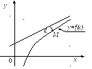
Рис. 5.10
Вертикальные асимптоты
Определение.
Прямая
![]() называетсявертикальной
называетсявертикальной
асимптотой графика
функции
![]() ,
,
если выполнено одно из условий:
![]() или
или
![]() (рис.5.11)
(рис.5.11)
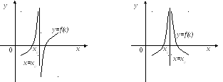
Рис. 5.11
Вертикальные
асимптоты, уравнение которых х=x0
, следует
искать в точках, где функция терпит
разрыв второго рода, или на концах ее
области определения, если концы не равны
![]() .
.
Если таких точек нет, то нет и вертикальных
асимптот.
Например, для
кривой
![]() ,
,
вертикальной асимптотой будет прямая![]() ,
,
так как![]() ,
,![]() .
.
Вертикальной асимптотой графика функции![]() является прямая
является прямая![]() (осьОу),
(осьОу),
поскольку
![]() .
.
Горизонтальные асимптоты
Определение.
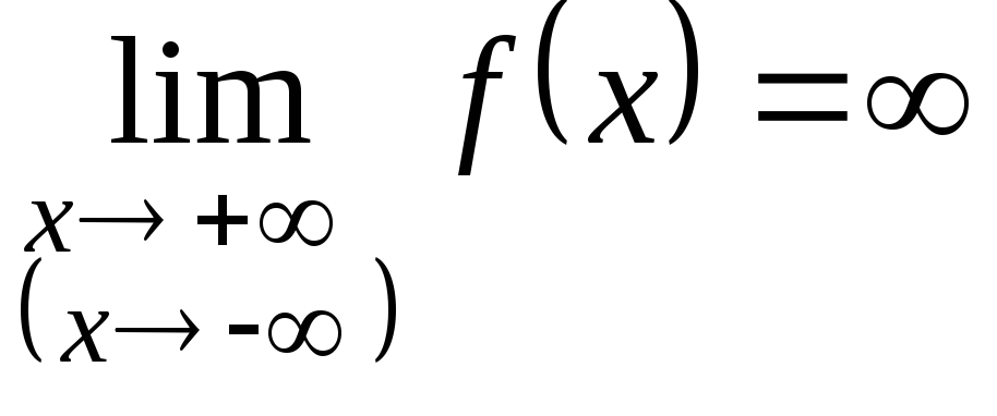
Если при
![]() (
(![]() )
)
функция![]() имеет конечный предел, равный числуb:
имеет конечный предел, равный числуb:
 ,
,
то прямая
![]() есть горизонтальная асимптота графика
есть горизонтальная асимптота графика
функции![]() .
.
Например, для
функции
![]() имеем
имеем
![]() ,
,
![]() .
.
Соответственно,
прямая
![]() − горизонтальная асимптота для правой
− горизонтальная асимптота для правой
ветви графика функции![]() ,
,
а прямая![]() − для левой ветви.
− для левой ветви.
В том случае, если
 ,
,
график функции не
имеет горизонтальных асимптот, но может
иметь наклонные.
Наклонные асимптоты
Определение.
Прямая
![]() называетсянаклонной
называетсянаклонной
асимптотой
графика функции
![]() при
при![]() (
(![]() ),
),
если выполняется равенство
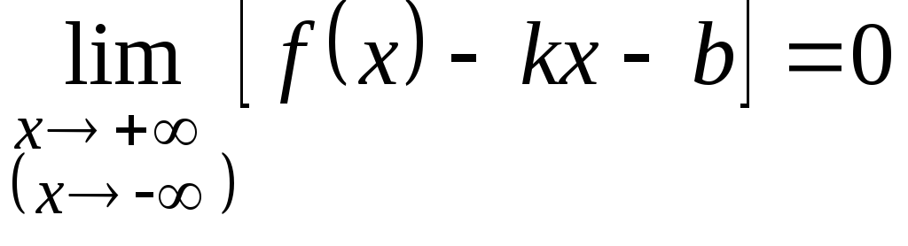 .
.
Наличие наклонной
асимптоты устанавливают с помощью
следующей теоремы.
Теорема.
Для того, чтобы
график функции
![]() имел при
имел при![]() (
(![]() )
)
наклонную асимптоту![]() ,
,
необходимо и достаточно, чтобы существовали
конечные пределы
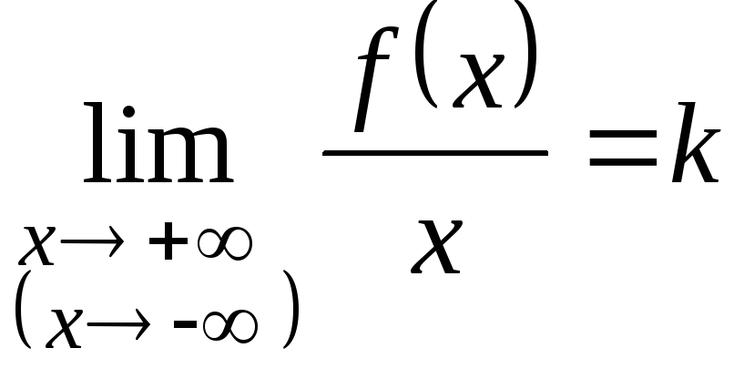 и
и
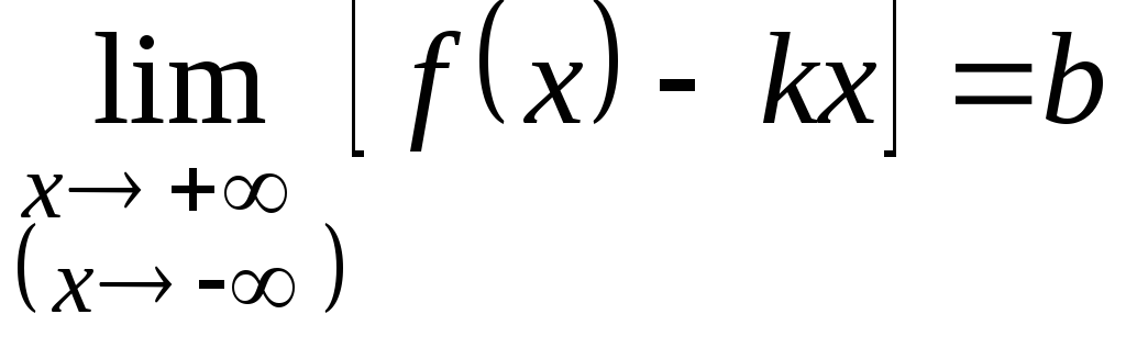 .
.
Если хотя бы один
из этих пределов не существует или равен
бесконечности, то кривая
![]() наклонной асимптоты не имеет.
наклонной асимптоты не имеет.
Замечания.
1. При отыскании
асимптот следует отдельно рассматривать
случаи
![]() и
и![]() .
.
2. Если
 и
и
 ,
,
то график функции
![]() имеет горизонтальную асимптоту
имеет горизонтальную асимптоту![]() .
.
3. Если
 и
и
 ,
,
то прямая
![]() (осьОх)
(осьОх)
является горизонтальной асимптотой
графика функции
![]() .
.
Из замечаний
следует, что горизонтальную асимптоту
можно рассматривать как частный случай
наклонной асимптоты при
![]() .
.
Поэтому при отыскании асимптот графика
функции рассматривают лишь два случая:
1) вертикальные
асимптоты,
2) наклонные
асимптоты.
Пример
Найти асимптоты
графика функции
![]() .
.
![]() .
.
1)
![]() − точка разрыва второго рода:
− точка разрыва второго рода:
![]() ,
,
![]() .
.
Прямая
![]() − вертикальная асимптота.
− вертикальная асимптота.
2)
![]() ,
,
![]() ,
,
![]() .
.
Прямая
![]() − горизонтальная асимптота. Наклонной
− горизонтальная асимптота. Наклонной
асимптоты нет.
5.6. Общая схема исследования функции и построение графика
В предыдущих
параграфах было показано, как с помощью
производных двух первых порядков
изучаются общие свойства функции.
Пользуясь результатами этого изучения,
можно составить представление о характере
функции и, в частности, построить ее
график.
Исследование
функции
![]() целесообразно проводить по следующей
целесообразно проводить по следующей
схеме.
-
Найти область
определения функции. -
Исследовать
функцию на четность и нечетность. -
Исследовать
функцию на периодичность. -
Найти точки
пересечения графика функции с осями
координат. -
Найти интервалы
знакопостоянства функции (интервалы,
на которых
 или).
или). -
Найти асимптоты
графика функции. -
Найти интервалы
монотонности и точки экстремума функции. -
Найти интервалы
выпуклости и вогнутости и точки перегиба
графика функции. -
Построить график
функции.
Пример
Исследовать функцию
![]() и построить ее график.
и построить ее график.
-
Область определения
функции
 .
. -
Функция нечетная:
 .
.
График функции симметричен относительно
начала координат -
Функция
непериодическая. -
Точки пересечения
с осями координат:
С осью Оу:
![]() ,
,
точка![]() .
.
С осью Ох:
![]() ,
,![]() ,
,![]() ,
,![]() .
.
-
Точки
 ,
, и
и разбивают осьОх
на четыре интервала.
![]() при
при
![]() ;
;
![]() при
при
![]() ;
;
![]() при
при
![]() ;
;
![]() при
при
![]() .
.
-
Так как функция
является непрерывной, то ее график не
имеет вертикальных асимптот.
![]() .
.
Наклонной и
горизонтальной асимптот нет.
-
 ,
,
![]() ,
,
![]() ,
,![]() − критические точки.
− критические точки.
![]() для
для
![]() «↑»,
«↑»,
![]() для
для
![]() «↓»,
«↓»,
![]() для
для
![]() «↑».
«↑».
Сведем данные в
таблицу.
|
х |
|
-1 |
|
1 |
|
|
|
+ |
0 |
− |
0 |
+ |
|
|
↑ (возрастает) |
mах 2 |
↓ (убывает) |
min -2 |
↑ (возрастает) |
![]() ,
,
![]() ;
;
точка
![]() − максимум;
− максимум;
точка
![]() − минимум.
− минимум.
-
 ,
,
 ,
, ,
, .
.
![]() при
при
![]() «
«![]() »;
»;
![]() при
при
![]() «
«![]() ».
».
|
х |
|
0 |
|
|
|
− |
0 |
+ |
|
|
(выпуклый) |
0 (точка перегиба) |
(вогнутый) |
Точка
![]() − точка перегиба.
− точка перегиба.
-
График функции
 (рис.5.12)
Рис. 5.12
Соседние файлы в предмете [НЕСОРТИРОВАННОЕ]
- #
- #
- #
- #
- #
- #
- #
- #
- #
- #
- #
- Понятие асимптоты
- Вертикальная асимптота
- Горизонтальная асимптота
- Наклонная асимптота
- Алгоритм исследования асимптотического поведения функции
- Примеры
п.1. Понятие асимптоты
Асимптота прямая, расстояние от которой до точки кривой стремится к нулю при удалении точки вдоль ветви кривой на бесконечность.
Различают вертикальные, горизонтальные и наклонные асимптоты.
Например:
п.2. Вертикальная асимптота
Вертикальная асимптота кривой (y=f(x)) имеет вид: (x=a)
где (a) — точка разрыва 2-го рода функции (f(x)), для которой хотя бы один односторонний предел существует и равен бесконечности.
Таким образом, практически каждой точке разрыва 2-го рода (см. §40 данного справочника) соответствует вертикальная асимптота.
Вертикальных асимптот может быть сколько угодно, в том числе, бесконечное множество (например, как у тангенса – см. §6 данного справочника).
Например:
Исследуем непрерывность функции (y=frac{1}{(x-1)(x+3)})
ОДЗ: (xne left{-3;1right})
(left{x_0=-3, x_1=1right}notin D) — точки не входят в ОДЗ, подозрительные на разрыв.
Исследуем (x_0=-3). Найдем односторонние пределы: begin{gather*} lim_{xrightarrow -3 -0}frac{1}{(x-1)(x+3)}=frac{1}{(-3-0-1)(-3-0+3)}=frac{1}{-4cdot(-0)}=+infty\ lim_{xrightarrow -3 +0}frac{1}{(x-1)(x+3)}=frac{1}{(-3+0-1)(-3+0+3)}=frac{1}{-4cdot(+0)}=-infty end{gather*} Односторонние пределы не равны и бесконечны.
Точка (x_0=-3) — точка разрыва 2-го рода.
Исследуем (x_1=1). Найдем односторонние пределы: begin{gather*} lim_{xrightarrow 1 -0}frac{1}{(x-1)(x+3)}=frac{1}{(1-0-1)(1-0+3)}=frac{1}{-0cdot 4}=-infty\ lim_{xrightarrow 1 +0}frac{1}{(x-1)(x+3)}=frac{1}{(1+0-1)(1+0+3)}=frac{1}{+0cdot 4}=+infty end{gather*} Односторонние пределы не равны и бесконечны.
Точка (x_1=1) — точка разрыва 2-го рода.
Вывод: у функции (y=frac{1}{(x-1)(x+3)}) две точки разрыва 2-го рода (left{x_0=-3, x_1=1right}), соответственно – две вертикальные асимптоты с уравнениями (x=-3) и (x=1).
п.3. Горизонтальная асимптота
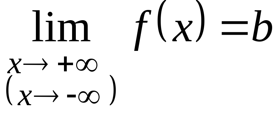
Горизонтальная асимптота кривой (y=f(x)) имеет вид: (y=b)
где (b) — конечный предел функции (f(x)) на бесконечности: (b=lim{xrightarrow pminfty}f(x), bneinfty)
Число горизонтальных асимптот не может быть больше двух.
Например:
Исследуем наличие горизонтальных асимптот у функции (y=frac{1}{(x-1)(x+3)})
Ищем предел функции на минус бесконечности: begin{gather*} lim_{xrightarrow -infty}frac{1}{(x-1)(x+3)}=frac{1}{(-infty)(-infty)}=+0 end{gather*} На минус бесконечности функция имеет конечный предел (b=0) и стремится к нему сверху (о чем свидетельствует символическая запись +0).
Ищем предел функции на плюс бесконечности: begin{gather*} lim_{xrightarrow +infty}frac{1}{(x-1)(x+3)}=frac{1}{(+infty)(+infty)}=+0 end{gather*} На плюс бесконечности функция имеет тот же конечный предел (b=0) и также стремится к нему сверху.
Вывод: у функции (y=frac{1}{(x-1)(x+3)}) одна горизонтальная асимптота (y=0). На плюс и минус бесконечности функция стремится к асимптоте сверху.
Итоговый график асимптотического поведения функции (y=frac{1}{(x-1)(x+3)}): 
п.4. Наклонная асимптота
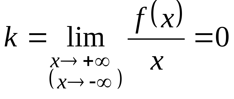
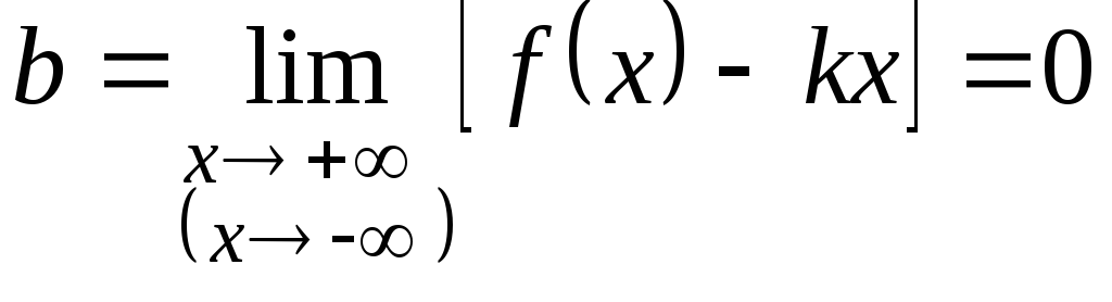
Наклонная асимптота кривой (y=f(x)) имеет вид: (y=kx+b) begin{gather*} k=lim_{xrightarrow pminfty}frac{f(x)}{x}, kne 0, kneinfty\ b=lim_{xrightarrow pminfty}(f(x)=kx) end{gather*}
Число наклонных асимптот не может быть больше двух.
Например:
Исследуем наличие наклонных асимптот у функции (y=frac{x^2+3}{x-1})
Найдем угловой коэффициент: begin{gather*} k_1=lim_{xrightarrow -infty}frac{y}{x}=lim_{xrightarrow -infty}frac{x^2+3}{x(x-1)}= lim_{xrightarrow -infty}frac{x^2+3}{x^2-x}=left[frac{infty}{infty}right]= lim_{xrightarrow -infty}frac{x^2left(1+frac{3}{x^2}right)}{x^2left(1-frac 1xright)}=\ =lim_{xrightarrow -infty}frac{1+frac{3}{x^2}}{1-frac1x}=frac{1+0}{1-0}=1\ k_2=lim_{xrightarrow +infty}frac{y}{x}=lim_{xrightarrow +infty}frac{x^2+3}{x(x-1)}=k_1=1 end{gather*} На плюс и минус бесконечности отношение функции к аргументу имеет один и тот же конечный предел (k=1).
Найдем свободный член: begin{gather*} b=lim_{xrightarrow pminfty}(y-kx)=lim_{xrightarrow pminfty}left(frac{x^2+3}{x-1}-1cdot xright)= lim_{xrightarrow pminfty}left(frac{x^2+3-x(x-1)}{x-1}right)=\ =lim_{xrightarrow pminfty}frac{x+3}{x-1}=left[frac{infty}{infty}right]=lim_{xrightarrow pminfty}frac{xleft(1+frac3xright)}{xleft(1-frac1xright)}=frac{1+0}{1-0}=1 end{gather*} Вывод: у функции (y=frac{x^2+3}{x-1}) одна наклонная асимптота (y=x+1). Функция стремится к асимптоте на плюс и минус бесконечности.
Чтобы построить график асимптотического поведения, заметим, что у функции (y=frac{x^2+3}{x-1}), очевидно, есть вертикальная асимптота x=1. При этом: begin{gather*} lim_{xrightarrow -1-0}frac{x^2+3}{x-1}=-infty, lim_{xrightarrow -1+0}frac{x^2+3}{x-1}=+infty end{gather*}
График асимптотического поведения функции (y=frac{x^2+3}{x-1}): 
п.5. Алгоритм исследования асимптотического поведения функции
На входе: функция (y=f(x))
Шаг 1. Поиск вертикальных асимптот
Исследовать функцию на непрерывность. Если обнаружены точки разрыва 2-го рода, у которых хотя бы один односторонний предел существует и бесконечен, сопоставить каждой такой точке вертикальную асимптоту. Если таких точек не обнаружено, вертикальных асимптот нет.
Шаг 2. Поиск горизонтальных асимптот
Найти пределы функции на плюс и минус бесконечности. Каждому конечному пределу сопоставить горизонтальную асимптоту. Если оба предела конечны и равны, у функции одна горизонтальная асимптота. Если оба предела бесконечны, горизонтальных асимптот нет.
Шаг 3. Поиск наклонных асимптот
Найти пределы отношения функции к аргументу на плюс и минус бесконечности.
Каждому конечному пределу k сопоставить наклонную асимптоту, найти b. Если только один предел конечен, у функции одна наклонная асимптота. Если оба значения k конечны и равны, и оба значения b равны, у функции одна наклонная асимптота. Если оба предела для k бесконечны, наклонных асимптот нет .
На выходе: множество всех асимптот данной функции.
п.6. Примеры
Пример 1. Исследовать асимптотическое поведение функции и построить схематический график:
a) ( y=frac{4x}{x^2-1} )
1) Вертикальные асимптоты
Точки, подозрительные на разрыв: (x=pm 1)
Односторонние пределы в точке (x=-1) begin{gather*} lim_{xrightarrow -1-0}frac{4x}{(x+1)(x-1)}=frac{4(-1-0)}{(-1-0+1)(-1-0-1)}=frac{-4}{-0cdot(-2)}=-infty\ lim_{xrightarrow -1+0}frac{4x}{(x+1)(x-1)}=frac{4(-1+0)}{(-1+0+1)(-1+0-1)}=frac{-4}{+0cdot(-2)}=+infty end{gather*} Точка (x=-1) — точка разрыва 2-го рода
Односторонние пределы в точке (x=1) begin{gather*} lim_{xrightarrow -1-0}frac{4x}{(x+1)(x-1)}=frac{4(1-0)}{(1-0+1)(1-0-1)}=frac{4}{2cdot(-0)}=-infty\ lim_{xrightarrow -1+0}frac{4x}{(x+1)(x-1)}=frac{4(1+0)}{(1+0+1)(1+0-1)}=frac{4}{2cdot(+0)}=+infty end{gather*} Точка (x=1) — точка разрыва 2-го рода
Функция имеет две вертикальные асимптоты (x=pm 1)
2) Горизонтальные асимптоты
Пределы функции на бесконечности: begin{gather*} b_1=lim_{xrightarrow -infty}frac{4x}{x^2-1}=left[frac{infty}{infty}right]=lim_{xrightarrow -infty}frac{x^2cdot frac4x}{x^2(1-frac{1}{x^2})}=lim_{xrightarrow -infty}frac{frac4x}{1-frac{1}{x^2}}=frac{-0}{1}=-0\ b_2=lim_{xrightarrow +infty}frac{4x}{x^2-1}=left[frac{infty}{infty}right]=lim_{xrightarrow +infty}frac{frac4x}{1-frac{1}{x^2}}=frac{+0}{1}=+0 end{gather*} Функция имеет одну горизонтальную асимптоту (y=0). На минус бесконечности функция стремится к асимптоте снизу, не плюс бесконечности – сверху.
3) Наклонные асимптоты
Ищем угловые коэффициенты: begin{gather*} k=lim_{xrightarrow pminfty}frac{4x}{x(x^2-1)}=lim_{xrightarrow pminfty}frac{4}{x^2-1}=frac{4}{infty}=0 end{gather*} Наклонных асимптот нет.
График асимптотического поведения функции (y=frac{4x}{x^2-1})
б) ( y=e^{frac{1}{x+3}} )
1) Вертикальные асимптоты
Точка, подозрительная на разрыв: (x=-3)
Односторонние пределы: begin{gather*} lim_{xrightarrow -3-0}e^{frac{1}{x+3}}=e^{frac{1}{-3-0)+3}}=e^{frac{1}{-0}}=e^infty=0\ lim_{xrightarrow -3+0}e^{frac{1}{x+3}}=e^{frac{1}{-3+0)+3}}=e^{frac{1}{+0}}=e^{+infty}=+infty end{gather*} Точка (x=-3) — точка разрыва 2-го рода
Функция имеет одну вертикальную асимптоту (x=2)
2) Горизонтальные асимптоты
Пределы функции на бесконечности: begin{gather*} b_1=lim_{xrightarrow -infty}e^{frac{1}{x+3}}=e^0=1\ b_2=lim_{xrightarrow +infty}e^{frac{1}{x+3}}=e^0=1\ b=b_1=b_2=1 end{gather*} Функция имеет одну горизонтальную асимптоту (y=1). Функция стремится к этой асимптоте на минус и плюс бесконечности.
3) Наклонные асимптоты
Ищем угловые коэффициенты: begin{gather*} k_1=lim_{xrightarrow -infty}frac{e^{frac{1}{x+3}}}{x}=frac{e^0}{-infty}=0\ k_2=lim_{xrightarrow +infty}frac{e^{frac{1}{x+3}}}{x}=frac{e^0}{+infty}=0 end{gather*} Наклонных асимптот нет.
График асимптотического поведения функции (y=e^{frac{1}{x+3}})
в) ( y=frac{x^3+x^2+x+1}{x^2-1} )
Заметим, что ( frac{x^3+x^2+x+1}{x^2-1}=frac{x^2(x+1)+(x+1)}{(x+1)(x-1)}=frac{(x^2)(x+1)}{(x+1)(x-1)}=frac{x^2+1}{x-1} ) $$ y=frac{x^3+x^2+x+1}{x^2-1}Leftrightarrow begin{cases} y=frac{x^2+1}{x-1}\ xne -1 end{cases} $$ График исходной функции совпадает с графиком функции (y=frac{x^2+1}{x-1}), из которого необходимо выколоть точку c абсциссой (x=-1).
1) Вертикальные асимптоты
Точки, подозрительные на разрыв: (x=pm 1)
Односторонние пределы в точке (x=-1) begin{gather*} lim_{xrightarrow -1-0}frac{x^3+x^2+x+1}{x^2-1}=lim_{xrightarrow -1-0}frac{x^2+1}{x-1}=frac{2}{-2}=-1\ lim_{xrightarrow -1+0}frac{x^3+x^2+x+1}{x^2-1}=lim_{xrightarrow -1-0}frac{x^2+1}{x-1}=frac{2}{-2}=-1 end{gather*} Точка (x=-1) — точка разрыва 1-го рода, устранимый разрыв («выколотая» точка).
Односторонние пределы в точке (x=1) begin{gather*} lim_{xrightarrow 1-0}frac{x^3+x^2+x+1}{x^2-1}=lim_{xrightarrow 1-0}frac{x^2+1}{x-1}=frac{2}{1-0-1}=frac{2}{-0}=-infty\ lim_{xrightarrow 1-0}frac{x^3+x^2+x+1}{x^2-1}=lim_{xrightarrow 1-0}frac{x^2+1}{x-1}=frac{2}{1+0-1}=frac{2}{+0}=+infty end{gather*} Точка (x=1) — точка разрыва 2-го рода
Функция имеет одну вертикальную асимптоту (x=1)
2) Горизонтальные асимптоты
Пределы функции на бесконечности: begin{gather*} b_1=lim_{xrightarrow -infty}frac{x^2+1}{x-1}=left[frac{infty}{infty}right]=lim_{xrightarrow -infty}frac{x^2left(1+frac{1}{x^2}right)}{x^2left(frac1x-frac{1}{x^2}right)}=frac{1+0}{-0-0}=-infty\ b_2=lim_{xrightarrow +infty}frac{x^2+1}{x-1}=left[frac{infty}{infty}right]=lim_{xrightarrow +infty}frac{x^2left(1+frac{1}{x^2}right)}{x^2left(frac1x-frac{1}{x^2}right)}=frac{1+0}{0-0}=+infty end{gather*} Оба предела бесконечны.
Функция не имеет горизонтальных асимптот.
3) Наклонные асимптоты
Ищем угловые коэффициенты: begin{gather*} k_1=lim_{xrightarrow -infty}frac{x^2+1}{x(x-1)}=left[frac{infty}{infty}right]=lim_{xrightarrow -infty}frac{x^2left(1+frac{1}{x^2}right)}{x^2left(1-frac1xright)}=frac{1+0}{1-0}=1\ k_2=lim_{xrightarrow +infty}frac{x^2+1}{x(x-1)}=left[frac{infty}{infty}right]=lim_{xrightarrow +infty}frac{x^2left(1+frac{1}{x^2}right)}{x^2left(1-frac1xright)}=frac{1+0}{1-0}=1\ k=k_1=k_2=1 end{gather*} У функции есть одна наклонная асимптота с (k=1).
Ищем свободный член: begin{gather*} b=lim_{xrightarrow infty}(y-kx)= lim_{xrightarrow infty}left(frac{x^2+1}{x-1}-2right)= lim_{xrightarrow infty}frac{x^2+1-x^2+x}{x-1}= lim_{xrightarrow infty}frac{x+1}{x-1}=left[frac{infty}{infty}right]=\ =lim_{xrightarrow infty}frac{xleft(1+frac1xright)}{xleft(1-frac1xright)}=frac{1+0}{1-0}=1 end{gather*} Функция имеет одну наклонную асимптоту (y=x+1).
График асимптотического поведения функции (y=frac{x^3+x^2+x+1}{x^2-1})
г*) ( y=xe^{frac{1}{2-x}} )
1) Вертикальные асимптоты
Точка, подозрительная на разрыв: (x=2)
Односторонние пределы: begin{gather*} lim_{xrightarrow 2-0}xe^{frac{1}{2-x}}=(2-0)e^{frac{1}{2-(2-0)}}=2e^{frac{1}{+0}}=2e^{+infty}=+infty\ lim_{xrightarrow 2+0}xe^{frac{1}{2-x}}=(2+0)e^{frac{1}{2-(2+0)}}=2e^{frac{1}{-0}}=2e^{-infty}=-infty end{gather*} Точка (x=2) — точка разрыва 2-го рода.
Функция имеет одну вертикальную асимптоту (x=2)
2) Горизонтальные асимптоты
Пределы функции на бесконечности: begin{gather*} b_1=lim_{xrightarrow -infty}xe^{frac{1}{2-x}}=-inftycdot e^0=-infty\ b_2=lim_{xrightarrow +infty}xe^{frac{1}{2-x}}=+inftycdot e^0=+infty end{gather*} Оба предела бесконечны.
Функция не имеет горизонтальных асимптот.
3) Наклонные асимптоты
Ищем угловые коэффициенты: begin{gather*} k_1=lim_{xrightarrow -infty}frac{xe^{frac{1}{2-x}}}{x}=lim_{xrightarrow -infty}e^{frac{1}{2-x}}=e^0=1\ k_2=lim_{xrightarrow +infty}frac{xe^{frac{1}{2-x}}}{x}=lim_{xrightarrow +infty}e^{frac{1}{2-x}}=e^0=1\ k=k_1=k_2=1 end{gather*} У функции есть одна наклонная асимптота с (k=1).
Ищем свободный член: begin{gather*} b=lim_{xrightarrow infty}(y-kx)= lim_{xrightarrow infty}left(xe^{frac{1}{2-x}}-xright)=lim_{xrightarrow infty}xleft(e^{frac{1}{2-x}}-1right)=left[inftycdot 0right] end{gather*} Используем одно из следствий второго замечательного предела (см. §39 данного справочника): begin{gather*} lim_{xrightarrow 0}frac{e^x-1}{x}=1\ b=lim_{xrightarrow infty}xleft(e^{frac{1}{2-x}}-1right)= left[ begin{array}{l} t=frac{1}{2-x}\ trightarrow 0\ x=2-frac1t=frac{2t-1}{t} end{array} right]=\ =lim_{trightarrow 0}left(left(frac{2t-1}{t}right)(e^t-1)right)=lim_{trightarrow 0}(2t-1)cdot lim_{trightarrow 0}frac{e^t-1}{t}=-1cdot 1=-1 end{gather*} Функция имеет одну наклонную асимптоту (y=x-1).
График асимптотического поведения функции (y=xe^{frac{1}{2-x}})
Для поиска асимптот можно использовать следующий алгоритм:
1. Для поиска вертикальных асимптот находим точки, не принадлежащие области определения ( ) и проверяем следующее условие: если
  , то — вертикальная асимптота.
Вертикальных асимптот может быть одна, несколько или не быть совсем.
2. Для поиска горизонтальных асимптот находим  .
.
3. Для поиска наклонных асимптот находим  .
.
Если функция представляет собой отношение двух многочленов, то при наличии у функции горизонтальных асимптот наклонные асимптоты искать не будем — их нет. Рассмотрим примеры нахождения асимптот функции:

Пример №16.1.
Найдите асимптоты кривой 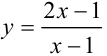 .
.
Решение:
1. Найдем область определения функции: 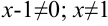 .
.
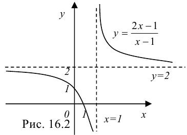
Проверим, является ли прямая  вертикальной асимптотой. Для этого вычислим предел функции в точке :
  .
.
Получили, что 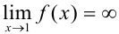 , следовательно, — вертикальная асимптота, х—>1
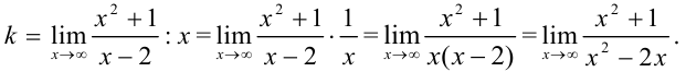
2. Для поиска горизонтальных асимптот находим :  .
.
Поскольку в пределе фигурирует неопределенность  , воспользуемся правилом Лопиталя:
 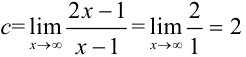 . Т.к.
  (число), то
  — горизонтальная асимптота.
Так как функция представляет собой отношение многочленов, то при наличии горизонтальных асимптот утверждаем, что наклонных асимптот нет.
Таким образом, данная функция имеет вертикальную асимптоту и горизонтальную асимптоту . Для наглядности график данной функции представлен на рис. 16.2.
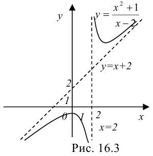
Пример №16.2.
Найдите асимптоты кривой 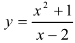 .
.
Решение:
1. Найдем область определения функции:  .
.
Проверим, является ли прямая  вертикальной асимптотой. Для этого вычислим предел функции в точке :
 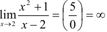 .
.
Получили, что  , следовательно, — вертикальная асимптота.
2. Для поиска горизонтальных асимптот находим : 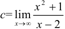 .
.
Поскольку в пределе фигурирует неопределенность , воспользуемся правилом Лопиталя: 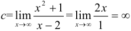 . Т.к.
  — бесконечность, то горизонтальных асимптот нет.
3. Для поиска наклонных асимптот находим  :
:
Получили неопределенность вида , воспользуемся правилом Лопиталя: 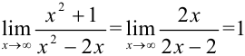 . Итак,
  . Найдем
  по формуле:
 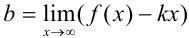 .
.
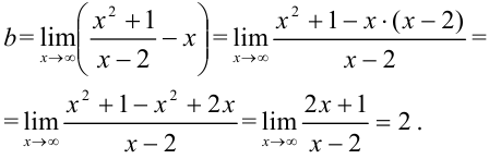
Получили, что  . Тогда
  — наклонная асимптота. В нашем случае она имеет вид:
  .
.
Таким образом, данная функция имеет вертикальную асимптоту и наклонную асимптоту . Для наглядности график функции представлен на рис. 16.3.
Эта лекция взята с главной страницы на которой находится курс лекций с теорией и примерами решения по всем разделам высшей математики:
Предмет высшая математика
Другие лекции по высшей математике, возможно вам пригодятся:

«Asymptotic» redirects here. Not to be confused with Asymptomatic.

The graph of a function with a horizontal (y = 0), vertical (x = 0), and oblique asymptote (purple line, given by y = 2x).

A curve intersecting an asymptote infinitely many times.
In analytic geometry, an asymptote () of a curve is a line such that the distance between the curve and the line approaches zero as one or both of the x or y coordinates tends to infinity. In projective geometry and related contexts, an asymptote of a curve is a line which is tangent to the curve at a point at infinity.[1][2]
The word asymptote is derived from the Greek ἀσύμπτωτος (asumptōtos) which means «not falling together», from ἀ priv. + σύν «together» + πτωτ-ός «fallen».[3] The term was introduced by Apollonius of Perga in his work on conic sections, but in contrast to its modern meaning, he used it to mean any line that does not intersect the given curve.[4]
There are three kinds of asymptotes: horizontal, vertical and oblique. For curves given by the graph of a function y = ƒ(x), horizontal asymptotes are horizontal lines that the graph of the function approaches as x tends to +∞ or −∞. Vertical asymptotes are vertical lines near which the function grows without bound. An oblique asymptote has a slope that is non-zero but finite, such that the graph of the function approaches it as x tends to +∞ or −∞.
More generally, one curve is a curvilinear asymptote of another (as opposed to a linear asymptote) if the distance between the two curves tends to zero as they tend to infinity, although the term asymptote by itself is usually reserved for linear asymptotes.
Asymptotes convey information about the behavior of curves in the large, and determining the asymptotes of a function is an important step in sketching its graph.[5] The study of asymptotes of functions, construed in a broad sense, forms a part of the subject of asymptotic analysis.
Introduction[edit]

The idea that a curve may come arbitrarily close to a line without actually becoming the same may seem to counter everyday experience. The representations of a line and a curve as marks on a piece of paper or as pixels on a computer screen have a positive width. So if they were to be extended far enough they would seem to merge, at least as far as the eye could discern. But these are physical representations of the corresponding mathematical entities; the line and the curve are idealized concepts whose width is 0 (see Line). Therefore, the understanding of the idea of an asymptote requires an effort of reason rather than experience.
Consider the graph of the function  shown in this section. The coordinates of the points on the curve are of the form
  where x is a number other than 0. For example, the graph contains the points (1, 1), (2, 0.5), (5, 0.2), (10, 0.1), … As the values of
  become larger and larger, say 100, 1,000, 10,000 …, putting them far to the right of the illustration, the corresponding values of
  , .01, .001, .0001, …, become infinitesimal relative to the scale shown. But no matter how large becomes, its reciprocal
  is never 0, so the curve never actually touches the x-axis. Similarly, as the values of become smaller and smaller, say .01, .001, .0001, …, making them infinitesimal relative to the scale shown, the corresponding values of , 100, 1,000, 10,000 …, become larger and larger. So the curve extends farther and farther upward as it comes closer and closer to the y-axis. Thus, both the x and y-axis are asymptotes of the curve. These ideas are part of the basis of concept of a limit in mathematics, and this connection is explained more fully below.[6]
Asymptotes of functions[edit]
The asymptotes most commonly encountered in the study of calculus are of curves of the form y = ƒ(x). These can be computed using limits and classified into horizontal, vertical and oblique asymptotes depending on their orientation. Horizontal asymptotes are horizontal lines that the graph of the function approaches as x tends to +∞ or −∞. As the name indicates they are parallel to the x-axis. Vertical asymptotes are vertical lines (perpendicular to the x-axis) near which the function grows without bound. Oblique asymptotes are diagonal lines such that the difference between the curve and the line approaches 0 as x tends to +∞ or −∞.
Vertical asymptotes[edit]
The line x = a is a vertical asymptote of the graph of the function y = ƒ(x) if at least one of the following statements is true:


where  is the limit as x approaches the value a from the left (from lesser values), and
  is the limit as x approaches a from the right.
For example, if ƒ(x) = x/(x–1), the numerator approaches 1 and the denominator approaches 0 as x approaches 1. So


and the curve has a vertical asymptote x = 1.
The function ƒ(x) may or may not be defined at a, and its precise value at the point x = a does not affect the asymptote. For example, for the function

has a limit of +∞ as x → 0+, ƒ(x) has the vertical asymptote x = 0, even though ƒ(0) = 5. The graph of this function does intersect the vertical asymptote once, at (0, 5). It is impossible for the graph of a function to intersect a vertical asymptote (or a vertical line in general) in more than one point. Moreover, if a function is continuous at each point where it is defined, it is impossible that its graph does intersect any vertical asymptote.
A common example of a vertical asymptote is the case of a rational function at a point x such that the denominator is zero and the numerator is non-zero.
If a function has a vertical asymptote, then it isn’t necessarily true that the derivative of the function has a vertical asymptote at the same place. An example is
 at .
at .


This function has a vertical asymptote at  because

and
- .

The derivative of  is the function
- .

For the sequence of points
- for


that approaches  both from the left and from the right, the values
  are constantly
  . Therefore, both one-sided limits of
  at can be neither
  nor
nor  . Hence
  doesn’t have a vertical asymptote at .
Horizontal asymptotes[edit]
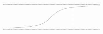
The arctangent function has two different asymptotes
Horizontal asymptotes are horizontal lines that the graph of the function approaches as x → ±∞. The horizontal line y = c is a horizontal asymptote of the function y = ƒ(x) if
- or .


In the first case, ƒ(x) has y = c as asymptote when x tends to −∞, and in the second ƒ(x) has y = c as an asymptote as x tends to +∞.
For example, the arctangent function satisfies
- and


So the line y = –π/2 is a horizontal asymptote for the arctangent when x tends to –∞, and y = π/2 is a horizontal asymptote for the arctangent when x tends to +∞.
Functions may lack horizontal asymptotes on either or both sides, or may have one horizontal asymptote that is the same in both directions. For example, the function ƒ(x) = 1/(x2+1) has a horizontal asymptote at y = 0 when x tends both to −∞ and +∞ because, respectively,

Other common functions that have one or two horizontal asymptotes include x ↦ 1/x (that has an hyperbola as it graph), the Gaussian function  the error function, and the logistic function.
Oblique asymptotes[edit]

In the graph of  , the y-axis (x = 0) and the line y = x are both asymptotes.
When a linear asymptote is not parallel to the x— or y-axis, it is called an oblique asymptote or slant asymptote. A function ƒ(x) is asymptotic to the straight line y = mx + n (m ≠ 0) if
![lim_{x to +infty}left[ f(x)-(mx+n)right] = 0 , mbox{ or } lim_{x to -infty}left[ f(x)-(mx+n)right] = 0.](https://wikimedia.org/api/rest_v1/media/math/render/svg/84dc363f0c720d0fe7f1c203c9292838937f0317)
In the first case the line y = mx + n is an oblique asymptote of ƒ(x) when x tends to +∞, and in the second case the line y = mx + n is an oblique asymptote of ƒ(x) when x tends to −∞.
An example is ƒ(x) = x + 1/x, which has the oblique asymptote y = x (that is m = 1, n = 0) as seen in the limits
![lim_{xtopminfty}left[f(x)-xright]](https://wikimedia.org/api/rest_v1/media/math/render/svg/765b8ffeff43ad3b7d5e8edba9a6124ce7c62f56)
![=lim_{xtopminfty}left[left(x+frac{1}{x}right)-xright]](https://wikimedia.org/api/rest_v1/media/math/render/svg/06a525e171c7838df9be10685a0fcba682e96a93)

Elementary methods for identifying asymptotes[edit]
The asymptotes of many elementary functions can be found without the explicit use of limits (although the derivations of such methods typically use limits).
General computation of oblique asymptotes for functions[edit]
The oblique asymptote, for the function f(x), will be given by the equation y = mx + n. The value for m is computed first and is given by

where a is either or depending on the case being studied. It is good practice to treat the two cases separately. If this limit doesn’t exist then there is no oblique asymptote in that direction.
Having m then the value for n can be computed by

where a should be the same value used before. If this limit fails to exist then there is no oblique asymptote in that direction, even should the limit defining m exist. Otherwise y = mx + n is the oblique asymptote of ƒ(x) as x tends to a.
For example, the function ƒ(x) = (2x2 + 3x + 1)/x has
- and then


so that y = 2x + 3 is the asymptote of ƒ(x) when x tends to +∞.
The function ƒ(x) = ln x has
- and then

- , which does not exist.

So y = ln x does not have an asymptote when x tends to +∞.
Asymptotes for rational functions[edit]
A rational function has at most one horizontal asymptote or oblique (slant) asymptote, and possibly many vertical asymptotes.
The degree of the numerator and degree of the denominator determine whether or not there are any horizontal or oblique asymptotes. The cases are tabulated below, where deg(numerator) is the degree of the numerator, and deg(denominator) is the degree of the denominator.
| deg(numerator)−deg(denominator) | Asymptotes in general | Example | Asymptote for example |
|---|---|---|---|
| < 0 | 
|

|
|
| = 0 | y = the ratio of leading coefficients | 
|

|
| = 1 | y = the quotient of the Euclidean division of the numerator by the denominator | 
|

|
| > 1 | none | 
|
no linear asymptote, but a curvilinear asymptote exists |
The vertical asymptotes occur only when the denominator is zero (If both the numerator and denominator are zero, the multiplicities of the zero are compared). For example, the following function has vertical asymptotes at x = 0, and x = 1, but not at x = 2.

Oblique asymptotes of rational functions[edit]

Black: the graph of  . Red: the asymptote
  . Green: difference between the graph and its asymptote for
When the numerator of a rational function has degree exactly one greater than the denominator, the function has an oblique (slant) asymptote. The asymptote is the polynomial term after dividing the numerator and denominator. This phenomenon occurs because when dividing the fraction, there will be a linear term, and a remainder. For example, consider the function

shown to the right. As the value of x increases, f approaches the asymptote y = x. This is because the other term, 1/(x+1), approaches 0.
If the degree of the numerator is more than 1 larger than the degree of the denominator, and the denominator does not divide the numerator, there will be a nonzero remainder that goes to zero as x increases, but the quotient will not be linear, and the function does not have an oblique asymptote.
Transformations of known functions[edit]
If a known function has an asymptote (such as y=0 for f(x)=ex), then the translations of it also have an asymptote.
- If x=a is a vertical asymptote of f(x), then x=a+h is a vertical asymptote of f(x—h)
- If y=c is a horizontal asymptote of f(x), then y=c+k is a horizontal asymptote of f(x)+k
If a known function has an asymptote, then the scaling of the function also have an asymptote.
- If y=ax+b is an asymptote of f(x), then y=cax+cb is an asymptote of cf(x)
For example, f(x)=ex-1+2 has horizontal asymptote y=0+2=2, and no vertical or oblique asymptotes.
General definition[edit]

(sec(t), cosec(t)), or x2 + y2 = (xy)2, with 2 horizontal and 2 vertical asymptotes.
Let A : (a,b) → R2 be a parametric plane curve, in coordinates A(t) = (x(t),y(t)). Suppose that the curve tends to infinity, that is:

A line ℓ is an asymptote of A if the distance from the point A(t) to ℓ tends to zero as t → b.[7] From the definition, only open curves that have some infinite branch can have an asymptote. No closed curve can have an asymptote.
For example, the upper right branch of the curve y = 1/x can be defined parametrically as x = t, y = 1/t (where t > 0). First, x → ∞ as t → ∞ and the distance from the curve to the x-axis is 1/t which approaches 0 as t → ∞. Therefore, the x-axis is an asymptote of the curve. Also, y → ∞ as t → 0 from the right, and the distance between the curve and the y-axis is t which approaches 0 as t → 0. So the y-axis is also an asymptote. A similar argument shows that the lower left branch of the curve also has the same two lines as asymptotes.
Although the definition here uses a parameterization of the curve, the notion of asymptote does not depend on the parameterization. In fact, if the equation of the line is  then the distance from the point A(t) = (x(t),y(t)) to the line is given by

if γ(t) is a change of parameterization then the distance becomes

which tends to zero simultaneously as the previous expression.
An important case is when the curve is the graph of a real function (a function of one real variable and returning real values). The graph of the function y = ƒ(x) is the set of points of the plane with coordinates (x,ƒ(x)). For this, a parameterization is

This parameterization is to be considered over the open intervals (a,b), where a can be −∞ and b can be +∞.
An asymptote can be either vertical or non-vertical (oblique or horizontal). In the first case its equation is x = c, for some real number c. The non-vertical case has equation y = mx + n, where m and  are real numbers. All three types of asymptotes can be present at the same time in specific examples. Unlike asymptotes for curves that are graphs of functions, a general curve may have more than two non-vertical asymptotes, and may cross its vertical asymptotes more than once.
Curvilinear asymptotes[edit]

x2+2x+3 is a parabolic asymptote to (x3+2x2+3x+4)/x
Let A : (a,b) → R2 be a parametric plane curve, in coordinates A(t) = (x(t),y(t)), and B be another (unparameterized) curve. Suppose, as before, that the curve A tends to infinity. The curve B is a curvilinear asymptote of A if the shortest distance from the point A(t) to a point on B tends to zero as t → b. Sometimes B is simply referred to as an asymptote of A, when there is no risk of confusion with linear asymptotes.[8]
For example, the function

has a curvilinear asymptote y = x2 + 2x + 3, which is known as a parabolic asymptote because it is a parabola rather than a straight line.[9]
Asymptotes and curve sketching[edit]
Asymptotes are used in procedures of curve sketching. An asymptote serves as a guide line to show the behavior of the curve towards infinity.[10] In order to get better approximations of the curve, curvilinear asymptotes have also been used [11] although the term asymptotic curve seems to be preferred.[12]
Algebraic curves[edit]

The asymptotes of an algebraic curve in the affine plane are the lines that are tangent to the projectivized curve through a point at infinity.[13] For example, one may identify the asymptotes to the unit hyperbola in this manner. Asymptotes are often considered only for real curves,[14] although they also make sense when defined in this way for curves over an arbitrary field.[15]
A plane curve of degree n intersects its asymptote at most at n−2 other points, by Bézout’s theorem, as the intersection at infinity is of multiplicity at least two. For a conic, there are a pair of lines that do not intersect the conic at any complex point: these are the two asymptotes of the conic.
A plane algebraic curve is defined by an equation of the form P(x,y) = 0 where P is a polynomial of degree n

where Pk is homogeneous of degree k. Vanishing of the linear factors of the highest degree term Pn defines the asymptotes of the curve: setting Q = Pn, if Pn(x, y) = (ax − by) Qn−1(x, y), then the line

is an asymptote if  and
and  are not both zero. If
  and
and  , there is no asymptote, but the curve has a branch that looks like a branch of parabola. Such a branch is called a parabolic branch, even when it does not have any parabola that is a curvilinear asymptote. If
  the curve has a singular point at infinity which may have several asymptotes or parabolic branches.
Over the complex numbers, Pn splits into linear factors, each of which defines an asymptote (or several for multiple factors). Over the reals, Pn splits in factors that are linear or quadratic factors. Only the linear factors correspond to infinite (real) branches of the curve, but if a linear factor has multiplicity greater than one, the curve may have several asymptotes or parabolic branches. It may also occur that such a multiple linear factor corresponds to two complex conjugate branches, and does not corresponds to any infinite branch of the real curve. For example, the curve x4 + y2 — 1 = 0 has no real points outside the square  , but its highest order term gives the linear factor x with multiplicity 4, leading to the unique asymptote x=0.
Asymptotic cone[edit]

Hyperbolas, obtained cutting the same right circular cone with a plane and their asymptotes.
The hyperbola

has the two asymptotes

The equation for the union of these two lines is

Similarly, the hyperboloid

is said to have the asymptotic cone[16][17]

The distance between the hyperboloid and cone approaches 0 as the distance from the origin approaches infinity.
More generally, consider a surface that has an implicit equation

where the  are homogeneous polynomials of degree
  and
and  . Then the equation
  defines a cone which is centered at the origin. It is called an asymptotic cone, because the distance to the cone of a point of the surface tends to zero when the point on the surface tends to infinity.
See also[edit]
- Big O notation
References[edit]
- General references
- Kuptsov, L.P. (2001) [1994], «Asymptote», Encyclopedia of Mathematics, EMS Press
- Specific references
- ^ Williamson, Benjamin (1899), «Asymptotes», An elementary treatise on the differential calculus
- ^ Nunemacher, Jeffrey (1999), «Asymptotes, Cubic Curves, and the Projective Plane», Mathematics Magazine, 72 (3): 183–192, CiteSeerX 10.1.1.502.72, doi:10.2307/2690881, JSTOR 2690881
- ^ Oxford English Dictionary, second edition, 1989.
- ^ D.E. Smith, History of Mathematics, vol 2 Dover (1958) p. 318
- ^ Apostol, Tom M. (1967), Calculus, Vol. 1: One-Variable Calculus with an Introduction to Linear Algebra (2nd ed.), New York: John Wiley & Sons, ISBN 978-0-471-00005-1, §4.18.
- ^ Reference for section: «Asymptote» The Penny Cyclopædia vol. 2, The Society for the Diffusion of Useful Knowledge (1841) Charles Knight and Co., London p. 541
- ^ Pogorelov, A. V. (1959), Differential geometry, Translated from the first Russian ed. by L. F. Boron, Groningen: P. Noordhoff N. V., MR 0114163, §8.
- ^ Fowler, R. H. (1920), The elementary differential geometry of plane curves, Cambridge, University Press, hdl:2027/uc1.b4073882, ISBN 0-486-44277-2, p. 89ff.
- ^ William Nicholson, The British enciclopaedia, or dictionary of arts and sciences; comprising an accurate and popular view of the present improved state of human knowledge, Vol. 5, 1809
- ^ Frost, P. An elementary treatise on curve tracing (1918) online
- ^ Fowler, R. H. The elementary differential geometry of plane curves Cambridge, University Press, 1920, pp 89ff.(online at archive.org)
- ^ Frost, P. An elementary treatise on curve tracing, 1918, page 5
- ^ C.G. Gibson (1998) Elementary Geometry of Algebraic Curves, § 12.6 Asymptotes, Cambridge University Press ISBN 0-521-64140-3,
- ^ Coolidge, Julian Lowell (1959), A treatise on algebraic plane curves, New York: Dover Publications, ISBN 0-486-49576-0, MR 0120551, pp. 40–44.
- ^ Kunz, Ernst (2005), Introduction to plane algebraic curves, Boston, MA: Birkhäuser Boston, ISBN 978-0-8176-4381-2, MR 2156630, p. 121.
- ^ L.P. Siceloff, G. Wentworth, D.E. Smith Analytic geometry (1922) p. 271
- ^ P. Frost Solid geometry (1875) This has a more general treatment of asymptotic surfaces.
External links[edit]
- Asymptote at PlanetMath.
- Hyperboloid and Asymptotic Cone, string surface model, 1872 Archived 2012-02-15 at the Wayback Machine from the Science Museum