Как найти число разбиений числа - Исправление недочетов и поиск решений вместе с Examum.ru

Материал из Викиконспекты

Перейти к: навигация, поиск

Задача:

По заданному числу найти количество его различных разбиений на положительные слагаемые^[1] так, что при всех .

Содержание

1 Алгоритм за O(N³)
2 Алгоритм за O(N²)
3 Алгоритм за O(N^3/2)
4 Примечания
5 См. также
6 Источники информации

Алгоритм за O(N³)

Пусть — количество разбиений числа на слагаемых, каждое из которых не превосходит .
Имеет место следующее рекуррентное соотношение:

Рассмотрим множество разбиений числа на слагаемых, каждое из которых не больше . Разделим его на две непересекающиеся группы — в первой будут все
разбиения, которые не содержат в качестве старшего слагаемого . Таких разбиений . Во второй — все разбиения со старшим слагаемым . Их столько же, сколько разбиений числа на слагаемое, каждое из которых не больше , то есть .

Количество всех разбиений числа равно . Реализация данного алгоритма методом динамического программирования с меморизацией будет иметь асимптотику .

Алгоритм за O(N²)

Обозначим — количество разбиений числа на слагаемые, каждое из которых не превосходит . Оно удовлетворяет следующей рекурентной формуле:

Заметим, что нам не нужно считать количество слагаемых в разбиении. Достаточно посчитать — количество разбиений числа на произвольное количество слагаемых, каждое из которых не больше . Рассмотрим множество таких разбиений. Разделим его на две непересекающиеся группы. В первую войдут те разбиения, в которых отсутствует слагаемое . Очевидно, таких разбиений . Во второй группе — те разбиения, в которые слагаемое вошло. Их количество совпадает с количеством разбиений числа на слагаемые, каждое из которых не превосходит , и равно .

Количество всех разбиений числа равно . Асимптотика .

Алгоритм за O(N^3/2)

Рассмотрим алгоритм нахождения количества разбиений числа на слагаемые, который работает за .

Итак, обозначим количество таких разбиений за .

Рассмотрим следующее бесконечное произведение:

После раскрытия скобок каждый член произведения получается в результате умножения мономов (одночленов), взятых по одному из каждой скобки. Если в первой скобке взять , во второй — и т.д., то их произведение будет равно Значит, после раскрытия скобок получится сумма мономов вида .

Можно увидеть, что встретится в полученной бесконечной сумме столько раз, сколькими способами можно представить как сумму Каждому такому представлению отвечает разбиение числа на единиц, двоек и т.д. Таким образом, очевидно, получаются все разбиения, так как из первой скобки мы можем взять любое , где то есть произвольное количество единиц в нашем разбиении. Аналогично, мы можем взять произвольное количество двоек и т.д. Но при раскрытии скобок мы находим произведения всех возможных комбинации множителей из разных скобок. Поэтому коэффициент при равен числу разбиений .

Посмотрим теперь на выражения в скобках. Каждое из них — бесконечная геометрическая прогрессия. Полагая , по формуле ее суммирования:

Запишем теперь производящую функцию последовательности :

Рассмотрим произведение , т.е. знаменатель правой части формулы . Раскрывая в нём скобки, получим следующий результат:

Показатели степеней в правой части — пятиугольные числа^[2], т.е. числа вида , а знаки при соответствующих мономах равны . Исходя из этого наблюдения, Эйлер предположил, что должна быть верна следующая теорема, впоследствии названная его именем.

Теорема (Пентагональная теорема Эйлера):

Доказательство:

Раскроем в этом произведении первые скобки. Мы получим выражение

где в квадратной скобке точками обозначены слагаемые, содержащие в более высокой степени, чем . Не будем выписывать эти члены, так как после умножения квадратной скобки на , и т.д. они изменятся. Выписанные же члены больше меняться не будут. Поэтому, если раскрыть все скобки, то получится бесконечный ряд, первые члены которого имеют вид

Анализируя этот ряд, Эйлер пришел к выводу, что, если превратить бесконечное произведение

в ряд, то в этом ряду отличны от нуля лишь слагаемые, вида , где — натуральное число.

При раскрытии скобок в исходном произведении слагаемое встретится столько раз, сколькими способами можно разбить число на различные слагаемые. При этом, если число слагаемых четно, то появляется , а если это число нечетно, то появляется . Например, разбиению соответствует слагаемое а разбиению — слагаемое . Таким образом, коэффициент при в разложении в ряд равен разности между количеством разбиений на четное число различных слагаемых и количеством разбиений на нечетное число различных слагаемых. Тогда теорему можно переформулировать следующим образом:

Теорема (Переформулировка пентагональной теоремы):

Если число не может быть представлено в виде , то оно имеет одинаковое количество разбиений на четное и на нечетное число различных слагаемых. А для чисел вида разность между этими количествами равна .

Иными словами, если четно, то на одно больше разбиений на четное число слагаемых, а если нечетно, то на одно больше разбиений на нечетное число слагаемых. Докажем эту теорему с помощью диаграмм Юнга^[3]. Покажем несколько способов превращения диаграммы с четным числом строк диаграмму из стольких же точек с нечетным числом строк и обратно.

Так как мы рассматриваем лишь разбиения на различные слагаемые, то диаграммы таких разбиений состоят из нескольких трапеций, поставленных друг на друга. Обозначим число точек в верхней строке диаграммы через , а число строк нижней трапеции через (на рис. 1 слева изображена диаграмма, для которой , ).

Преобразование 1. Предположим, что диаграмма содержит не менее двух трапеций, причем . В этом случае отбросим первую строку из точек, но удлиним последние строк нижней трапеции на одну точку (рис. 1). После этого общее число точек не изменится, все строки окажутся различной длины, но четность числа строк изменится.

Точно такое же преобразование можно сделать, если диаграмма состоит из одной трапеции, но . Стираем верхнюю строку и к нижним строчкам приписываем точек.

Преобразование 2.Пусть теперь диаграмма опять содержит не менее двух трапеций, но . Тогда от каждой строки последней трапеции возьмем по одной точке и составим из них первую строку (из точек) новой диаграммы. Это можно сделать, так как , и поэтому составленная строка короче первой строки исходной диаграммы. Кроме того, так как мы взяли все строки будут иметь различную длину. Наконец, новая диаграмма содержит столько же точек, что и исходная, но четность числа строк изменилась — новая диаграмма содержит еще одну строку.

Преобразование 2 допускают и диаграммы, состоящие из одной трапеции, если (появляющаяся первая строка состоит из точек, она должна быть короче бывшей первой строки, уменьшившейся до точки).

Легко видеть, что описанные преобразования взаимно обратны — если сначала сделать одно из них, а потом второе, то снова получим исходную диаграмму. Кроме того, для каждой диаграммы может быть допустимо лишь одно из этих преобразований. Таким образом, диаграммы разбиений числа , допускающие одно из этих преобразований, распадаются на пары диаграмм с четным и нечетным числом строк, поэтому их одинаковое число.

Осталось выяснить, какие же диаграммы не допускают ни одного из описанных преобразований. Ясно, что эти диаграммы состоят из одной трапеции, причем для них либо , либо . В первом случае диаграмма содержит

точек, а во втором — на точек больше, т.е. .

Приведенные рассуждения показывают, что если не является числом вида , то оно имеет поровну разбиений на четное и нечетное число различных слагаемых.

Очевидно также, что равенства и одновременно выполняться не могут, поэтому если , то без пары останется ровно одна диаграмма, не допускающая преобразования и имеющая строк (слагаемых ). Если — четное число, то разбиений на четное число слагаемых окажется на больше, чем на нечетное число слагаемых. Если же — нечетное число, то на больше будет разбиений на нечетное число слагаемых. Теорема доказана.

Умножим обе части равенства на и воспользуемся пентагональной теоремой:

Начнем раскрывать скобки, для наглядности мономы с одинаковыми степенями пишем друг под другом:

Так как , то оно сокращается с единицей справа. Так что, чтобы выражение было удовлетворено при любом , все коэффициенты должны быть равны . Поэтому:

Получаем формулу Эйлера, позволяющую последовательно находить числа :

Асимптотика получается следующим образом. Так как , то получаем порядка , а так как находим -е число, то получаем .

Примечания

↑ Последовательность 000041 на OEIS
↑ Википедия — Пятиугольные числа
↑ Википедия — Диаграммы Юнга

См. также

Числа Стирлинга первого рода
Числа Стирлинга второго рода
Производящая функция

Источники информации

Wikipedia — Pentagonal number theorem
Вайнштейн Ф., Разбиение чисел. Журнал «Квант» № 11, 1988 год
Н.Я. Виленкин «Комбинаторика», 2007. стр. 138-141.

Источник

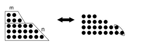
The values of the partition function (1, 2, 3, 5, 7, 11, 15, and 22) can be determined by counting the Young diagrams for the partitions of the numbers from 1 to 8.

In number theory, the partition function p(n) represents the number of possible partitions of a non-negative integer n. For instance, p(4) = 5 because the integer 4 has the five partitions 1 + 1 + 1 + 1, 1 + 1 + 2, 1 + 3, 2 + 2, and 4.

No closed-form expression for the partition function is known, but it has both asymptotic expansions that accurately approximate it and recurrence relations by which it can be calculated exactly. It grows as an exponential function of the square root of its argument. The multiplicative inverse of its generating function is the Euler function; by Euler’s pentagonal number theorem this function is an alternating sum of pentagonal number powers of its argument.

Srinivasa Ramanujan first discovered that the partition function has nontrivial patterns in modular arithmetic, now known as Ramanujan’s congruences. For instance, whenever the decimal representation of n ends in the digit 4 or 9, the number of partitions of n will be divisible by 5.

Definition and examples[edit]

For a positive integer n, p(n) is the number of distinct ways of representing n as a sum of positive integers. For the purposes of this definition, the order of the terms in the sum is irrelevant: two sums with the same terms in a different order are not considered to be distinct.

By convention p(0) = 1, as there is one way (the empty sum) of representing zero as a sum of positive integers. Furthermore p(n) = 0 when n is negative.

The first few values of the partition function, starting with p(0) = 1, are:

1, 1, 2, 3, 5, 7, 11, 15, 22, 30, 42, 56, 77, 101, 135, 176, 231, 297, 385, 490, 627, 792, 1002, 1255, 1575, 1958, 2436, 3010, 3718, 4565, 5604, … (sequence A000041 in the OEIS).

Some exact values of p(n) for larger values of n include:^[1]

${displaystyle {begin{aligned}p(100)&=190,!569,!292\p(1000)&=24,!061,!467,!864,!032,!622,!473,!692,!149,!727,!991approx 2.40615times 10^{31}\p(10000)&=36,!167,!251,!325,!dots ,!906,!916,!435,!144approx 3.61673times 10^{106}end{aligned}}}$

As of June 2022, the largest known prime number among the values of p(n) is p(1289844341), with 40,000 decimal digits.^[2]^[3] Until March 2022, this was also the largest prime that has been proved using elliptic curve primality proving.^[4]

Generating function[edit]

Using Euler’s method to find p(40): A ruler with plus and minus signs (grey box) is slid downwards, the relevant terms added or subtracted. The positions of the signs are given by differences of alternating natural (blue) and odd (orange) numbers. In the SVG file, hover over the image to move the ruler.

The generating function for p(n) is given by^[5]

${displaystyle {begin{aligned}sum _{n=0}^{infty }p(n)x^{n}&=prod _{k=1}^{infty }left({frac {1}{1-x^{k}}}right)\&=left(1+x+x^{2}+x^{3}+cdots right)left(1+x^{2}+x^{4}+x^{6}+cdots right)left(1+x^{3}+x^{6}+x^{9}+cdots right)cdots \&={frac {1}{1-x-x^{2}+x^{5}+x^{7}-x^{12}-x^{15}+x^{22}+x^{26}-cdots }}\&=1{Big /}sum _{k=-infty }^{infty }(-1)^{k}x^{k(3k-1)/2}.end{aligned}}}$

The equality between the products on the first and second lines of this formula
is obtained by expanding each factor ${displaystyle 1/(1-x^{k})}$ into the geometric series ${displaystyle (1+x^{k}+x^{2k}+x^{3k}+cdots ).}$
To see that the expanded product equals the sum on the first line,
apply the distributive law to the product. This expands the product into a sum of monomials of the form ${displaystyle x^{a_{1}}x^{2a_{2}}x^{3a_{3}}cdots }$ for some sequence of coefficients
$a_{i}$ , only finitely many of which can be non-zero.
The exponent of the term is ${textstyle n=sum ia_{i}}$ , and this sum can be interpreted as a representation of as a partition into $a_{i}$ copies of each number . Therefore, the number of terms of the product that have exponent is exactly p(n) , the same as the coefficient of $x^{n}$ in the sum on the left.
Therefore, the sum equals the product.

The function that appears in the denominator in the third and fourth lines of the formula is the Euler function. The equality between the product on the first line and the formulas in the third and fourth lines is Euler’s pentagonal number theorem.
The exponents of in these lines are the pentagonal numbers ${displaystyle P_{k}=k(3k-1)/2}$ for (generalized somewhat from the usual pentagonal numbers, which come from the same formula for the positive values of ). The pattern of positive and negative signs in the third line comes from the term $(-1)^{k}$ in the fourth line: even choices of produce positive terms, and odd choices produce negative terms.

More generally, the generating function for the partitions of into numbers selected from a set of positive integers can be found by taking only those terms in the first product for which . This result is due to Leonhard Euler.^[6] The formulation of Euler’s generating function is a special case of a -Pochhammer symbol and is similar to the product formulation of many modular forms, and specifically the Dedekind eta function.

Recurrence relations[edit]

The same sequence of pentagonal numbers appears in a recurrence relation for the partition function:^[7]

${displaystyle {begin{aligned}p(n)&=sum _{kin mathbb {Z} setminus {0}}(-1)^{k+1}p(n-k(3k-1)/2)\&=p(n-1)+p(n-2)-p(n-5)-p(n-7)+p(n-12)+p(n-15)-p(n-22)-cdots end{aligned}}}$

As base cases, p(0) is taken to equal , and p(k) is taken to be zero for negative . Although the sum on the right side appears infinite, it has only finitely many nonzero terms,
coming from the nonzero values of in the range

${displaystyle -{frac {{sqrt {24n+1}}-1}{6}}leq kleq {frac {{sqrt {24n+1}}+1}{6}}.}$

Another recurrence relation for p(n) can be given in terms of the sum of divisors function σ:^[8]

${displaystyle p(n)={frac {1}{n}}sum _{k=0}^{n-1}sigma (n-k)p(k).}$

If q(n) denotes the number of partitions of with no repeated parts then it follows by splitting each partition into its even parts and odd parts, and dividing the even parts by two, that^[9]

${displaystyle p(n)=sum _{k=0}^{leftlfloor n/2rightrfloor }q(n-2k)p(k).}$

Congruences[edit]

Srinivasa Ramanujan is credited with discovering that the partition function has nontrivial patterns in modular arithmetic.
For instance the number of partitions is divisible by five whenever the decimal representation of ends in the digit 4 or 9, as expressed by the congruence^[10]

For instance, the number of partitions for the integer 4 is 5.
For the integer 9, the number of partitions is 30; for 14 there are 135 partitions. This congruence is implied by the more general identity

${displaystyle sum _{k=0}^{infty }p(5k+4)x^{k}=5~{frac {(x^{5})_{infty }^{5}}{(x)_{infty }^{6}}},}$

also by Ramanujan,^[11]^[12] where the notation ${displaystyle (x)_{infty }}$ denotes the product defined by

${displaystyle (x)_{infty }=prod _{m=1}^{infty }(1-x^{m}).}$

A short proof of this result can be obtained from the partition function generating function.

Ramanujan also discovered congruences modulo 7 and 11:^[10]

${displaystyle {begin{aligned}p(7k+5)&equiv 0{pmod {7}},\p(11k+6)&equiv 0{pmod {11}}.end{aligned}}}$

The first one comes from Ramanujan’s identity^[12]

${displaystyle sum _{k=0}^{infty }p(7k+5)x^{k}=7~{frac {(x^{7})_{infty }^{3}}{(x)_{infty }^{4}}}+49x~{frac {(x^{7})_{infty }^{7}}{(x)_{infty }^{8}}}.}$

Since 5, 7, and 11 are consecutive primes, one might think that there would be an analogous congruence for the next prime 13, for some a. However, there is no congruence of the form for any prime b other than 5, 7, or 11.^[13] Instead, to obtain a congruence, the argument of should take the form for some c>1 . In the 1960s, A. O. L. Atkin of the University of Illinois at Chicago discovered additional congruences of this form for small prime moduli. For example:

${displaystyle p(11^{3}cdot 13cdot k+237)equiv 0{pmod {13}}.}$

Ken Ono (2000) proved that there are such congruences for every prime modulus greater than 3. Later, Ahlgren & Ono (2001) showed there are partition congruences modulo every integer coprime to 6.^[14]^[15]

Approximation formulas[edit]

Approximation formulas exist that are faster to calculate than the exact formula given above.

An asymptotic expression for p(n) is given by

${displaystyle p(n)sim {frac {1}{4n{sqrt {3}}}}exp left({pi {sqrt {frac {2n}{3}}}}right)}$

This asymptotic formula was first obtained by G. H. Hardy and Ramanujan in 1918 and independently by J. V. Uspensky in 1920. Considering , the asymptotic formula gives about ${displaystyle 2.4402times 10^{31}}$ , reasonably close to the exact answer given above (1.415% larger than the true value).

Hardy and Ramanujan obtained an asymptotic expansion with this approximation as the first term:^[16]

${displaystyle p(n)sim {frac {1}{2pi {sqrt {2}}}}sum _{k=1}^{v}A_{k}(n){sqrt {k}}cdot {frac {d}{dn}}left({{frac {1}{sqrt {n-{frac {1}{24}}}}}exp left[{{frac {pi }{k}}{sqrt {{frac {2}{3}}left(n-{frac {1}{24}}right)}}},,,right]}right),}$

where

${displaystyle A_{k}(n)=sum _{0leq m<k,;(m,k)=1}e^{pi ileft(s(m,k)-2nm/kright)}.}$

Here, the notation means that the sum is taken only over the values of that are relatively prime to . The function is a Dedekind sum.

The error after terms is of the order of the next term, and may be taken to be of the order of . As an example, Hardy and Ramanujan showed that is the nearest integer to the sum of the first terms of the series.^[16]

In 1937, Hans Rademacher was able to improve on Hardy and Ramanujan’s results by providing a convergent series expression for p(n) . It is^[17]^[18]

${displaystyle p(n)={frac {1}{pi {sqrt {2}}}}sum _{k=1}^{infty }A_{k}(n){sqrt {k}}cdot {frac {d}{dn}}left({{frac {1}{sqrt {n-{frac {1}{24}}}}}sinh left[{{frac {pi }{k}}{sqrt {{frac {2}{3}}left(n-{frac {1}{24}}right)}}},,,right]}right).}$

The proof of Rademacher’s formula involves Ford circles, Farey sequences, modular symmetry and the Dedekind eta function.

It may be shown that the th term of Rademacher’s series is of the order

${displaystyle exp left({frac {pi }{k}}{sqrt {frac {2n}{3}}}right),}$

so that the first term gives the Hardy–Ramanujan asymptotic approximation.
Paul Erdős (1942) published an elementary proof of the asymptotic formula for p(n) .^[19]^[20]

Techniques for implementing the Hardy–Ramanujan–Rademacher formula efficiently on a computer are discussed by Johansson (2012), who shows that p(n) can be computed in time ${displaystyle O(n^{1/2+varepsilon })}$ for any . This is near-optimal in that it matches the number of digits of the result.^[21] The largest value of the partition function computed exactly is ${displaystyle p(10^{20})}$ , which has slightly more than 11 billion digits.^[22]

Strict partition function[edit]

Definition and properties[edit]

A partition in which no part occurs more than one is called strict, or is said to be a partition into distinct parts. The function q(n) gives the number of these strict partitions of the given sum n. For example, q(3) = 2 because the partitions 3 and 1 + 2 are strict, while the third partition 1 + 1 + 1 of 3 has repeated parts. The number q(n) is also equal to the number of partitions of n in which only odd summands are permitted.^[23]

Example values of q(n) and associated partitions

n	q(n)	Strict partitions	Partitions with only odd parts
0	1	() empty partition	() empty partition
1	1	1	1
2	1	2	1+1
3	2	1+2, 3	1+1+1, 3
4	2	1+3, 4	1+1+1+1, 1+3
5	3	2+3, 1+4, 5	1+1+1+1+1, 1+1+3, 5
6	4	1+2+3, 2+4, 1+5, 6	1+1+1+1+1+1, 1+1+1+3, 3+3, 1+5
7	5	1+2+4, 3+4, 2+5, 1+6, 7	1+1+1+1+1+1+1, 1+1+1+1+3, 1+3+3, 1+1+5, 7
8	6	1+3+4, 1+2+5, 3+5, 2+6, 1+7, 8	1+1+1+1+1+1+1+1, 1+1+1+1+1+3, 1+1+3+3, 1+1+1+5, 3+5, 1+7
9	8	2+3+4, 1+3+5, 4+5, 1+2+6, 3+6, 2+7, 1+8, 9	1+1+1+1+1+1+1+1+1, 1+1+1+1+1+1+3, 1+1+1+3+3, 3+3+3, 1+1+1+1+5, 1+3+5, 1+1+7, 9

Generating function[edit]

The generating function for the numbers q(n) is given by a simple infinite product:^[24]

${displaystyle sum _{n=0}^{infty }q(n)x^{n}=prod _{k=1}^{infty }(1+x^{n})=(x;x^{2})_{infty }^{-1},}$

where the notation ${displaystyle (a;b)_{infty }}$ represents the Pochhammer symbol ${displaystyle (a;b)_{infty }=prod _{k=0}^{infty }(1-ab^{k}).}$ From this formula, one may easily obtain the first few terms (sequence A000009 in the OEIS):

${displaystyle sum _{n=0}^{infty }q(n)x^{n}=1+1x+1x^{2}+2x^{3}+2x^{4}+3x^{5}+4x^{6}+5x^{7}+6x^{8}+8x^{9}+10x^{10}+ldots .}$

This series may also be written in terms of theta functions as

${displaystyle sum _{n=0}^{infty }q(n)x^{n}=vartheta _{00}(x)^{1/6}vartheta _{01}(x)^{-1/3}{biggl {}{frac {1}{16,x}}{bigl [}vartheta _{00}(x)^{4}-vartheta _{01}(x)^{4}{bigr ]}{biggr }}^{1/24},}$

where

${displaystyle vartheta _{00}(x)=1+2sum _{n=1}^{infty }x^{n^{2}}}$

and

${displaystyle vartheta _{01}(x)=1+2sum _{n=1}^{infty }(-1)^{n}x^{n^{2}}.}$

In comparison, the generating function of the regular partition numbers p(n) has this identity with respect to the theta function:

${displaystyle sum _{n=0}^{infty }p(n)x^{n}=(x;x)_{infty }^{-1}=vartheta _{00}(x)^{-1/6}vartheta _{01}(x)^{-2/3}{biggl {}{frac {1}{16,x}}{bigl [}vartheta _{00}(x)^{4}-vartheta _{01}(x)^{4}{bigr ]}{biggr }}^{-1/24}.}$

Identities about strict partition numbers[edit]

Following identity is valid for the Pochhammer products:

${displaystyle (x;x)_{infty }^{-1}=(x^{2};x^{2})_{infty }^{-1}(x;x^{2})_{infty }^{-1}}$

From this identity follows that formula:

${displaystyle {biggl [}sum _{n=0}^{infty }p(n)x^{n}{biggr ]}={biggl [}sum _{n=0}^{infty }p(n)x^{2n}{biggr ]}{biggl [}sum _{n=0}^{infty }q(n)x^{n}{biggr ]}}$

Therefore those two formulas are valid for the synthesis of the number sequence p(n):

${displaystyle p(2n)=sum _{k=0}^{n}p(n-k)q(2k)}$

${displaystyle p(2n+1)=sum _{k=0}^{n}p(n-k)q(2k+1)}$

In the following, two examples are accurately executed:

${displaystyle p(8)=sum _{k=0}^{4}p(4-k)q(2k)=}$

{displaystyle =p(4)q(0)+p(3)q(2)+p(2)q(4)+p(1)q(6)+p(0)q(8)=}

{displaystyle =5times 1+3times 1+2times 2+1times 4+1times 6=22}

${displaystyle p(9)=sum _{k=0}^{4}p(4-k)q(2k+1)=}$

{displaystyle =p(4)q(1)+p(3)q(3)+p(2)q(5)+p(1)q(7)+p(0)q(9)=}

{displaystyle =5times 1+3times 2+2times 3+1times 5+1times 8=30}

Restricted partition function[edit]

More generally, it is possible to consider partitions restricted to only elements of a subset A of the natural numbers (for example a restriction on the maximum value of the parts), or with a restriction on the number of parts or the maximum difference between parts. Each particular restriction gives rise to an associated partition function with specific properties. Some common examples are given below.

Euler and Glaisher’s theorem[edit]

Two important examples are the partitions restricted to only odd integer parts or only even integer parts, with the corresponding partition functions often denoted ${displaystyle p_{o}(n)}$ and ${displaystyle p_{e}(n)}$ .

A theorem from Euler shows that the number of strict partitions is equal to the number of partitions with only odd parts: for all n, ${displaystyle q(n)=p_{o}(n)}$ . This is generalized as Glaisher’s theorem, which states that the number of partitions with no more than d-1 repetitions of any part is equal to the number of partitions with no part divisible by d.

Gaussian binomial coefficient[edit]

If we denote the number of partitions of n in at most M parts, with each part smaller or equal to N, then the generating function of is the following Gaussian binomial coefficient:

${displaystyle sum _{n=0}^{infty }p(N,M,n)q^{n}={N+M choose M}_{q}={frac {(1-q^{N+M})(1-q^{N+M-1})cdots (1-q^{N+1})}{(1-q)(1-q^{2})cdots (1-q^{M})}}}$

Asymptotics[edit]

Some general results on the asymptotic properties of restricted partition functions are known. If p_A(n) is the partition function of partitions restricted to only elements of a subset A of the natural numbers, then:

If A possesses positive natural density α then ${displaystyle log p_{A}(n)sim C{sqrt {alpha n}}}$ , with $C=pi {sqrt {frac {2}{3}}}$

and conversely if this asymptotic property holds for p_A(n) then A has natural density α.^[25] This result was stated, with a sketch of proof, by Erdős in 1942.^[19]^[26]

If A is a finite set, this analysis does not apply (the density of a finite set is zero). If A has k elements whose greatest common divisor is 1, then^[27]

$p_{A}(n)=left(prod _{ain A}a^{-1}right)cdot {frac {n^{k-1}}{(k-1)!}}+O(n^{k-2}).$

References[edit]

^ Sloane, N. J. A. (ed.), «Sequence A070177», The On-Line Encyclopedia of Integer Sequences, OEIS Foundation
^ Caldwell, Chris K. (2017), The Top Twenty
^ «PrimePage Primes: p(1289844341)», primes.utm.edu, retrieved 30 June 2022
^ «The Top Twenty: Elliptic Curve Primality Proof», primes.utm.edu, retrieved 30 June 2022
^ Abramowitz, Milton; Stegun, Irene (1964), Handbook of Mathematical Functions with Formulas, Graphs, and Mathematical Tables, United States Department of Commerce, National Bureau of Standards, p. 825, ISBN 0-486-61272-4
^ Euler, Leonhard (1753), «De partitione numerorum», Novi Commentarii Academiae Scientiarum Petropolitanae (in Latin), 3: 125–169
^ Ewell, John A. (2004), «Recurrences for the partition function and its relatives», The Rocky Mountain Journal of Mathematics, 34 (2): 619–627, doi:10.1216/rmjm/1181069871, JSTOR 44238988, MR 2072798
^ Wilf, Herbert S. (1982), «What is an answer?», American Mathematical Monthly, 89 (5): 289–292, doi:10.2307/2321713, JSTOR 2321713, MR 0653502
^ Al, Busra; Alkan, Mustafa (2018), «A note on relations among partitions», Proc. Mediterranean Int. Conf. Pure & Applied Math. and Related Areas (MICOPAM 2018), pp. 35–39
^ ^a ^b Hardy, G. H.; Wright, E. M. (2008) [1938], An Introduction to the Theory of Numbers (6th ed.), Oxford University Press, p. 380, ISBN 978-0-19-921986-5, MR 2445243, Zbl 1159.11001
^ Berndt, Bruce C.; Ono, Ken (1999), «Ramanujan’s unpublished manuscript on the partition and tau functions with proofs and commentary» (PDF), The Andrews Festschrift (Maratea, 1998), Séminaire Lotharingien de Combinatoire, vol. 42, Art. B42c, 63, MR 1701582
^ ^a ^b Ono, Ken (2004), The web of modularity: arithmetic of the coefficients of modular forms and -series, CBMS Regional Conference Series in Mathematics, vol. 102, Providence, Rhode Island: American Mathematical Society, p. 87, ISBN 0-8218-3368-5, Zbl 1119.11026
^ Ahlgren, Scott; Boylan, Matthew (2003), «Arithmetic properties of the partition function» (PDF), Inventiones Mathematicae, 153 (3): 487–502, Bibcode:2003InMat.153..487A, doi:10.1007/s00222-003-0295-6, MR 2000466, S2CID 123104639
^ Ono, Ken (2000), «Distribution of the partition function modulo «, Annals of Mathematics, 151 (1): 293–307, arXiv:math/0008140, Bibcode:2000math……8140O, doi:10.2307/121118, JSTOR 121118, MR 1745012, S2CID 119750203, Zbl 0984.11050
^ Ahlgren, Scott; Ono, Ken (2001), «Congruence properties for the partition function» (PDF), Proceedings of the National Academy of Sciences, 98 (23): 12882–12884, Bibcode:2001PNAS…9812882A, doi:10.1073/pnas.191488598, MR 1862931, PMC 60793, PMID 11606715
^ ^a ^b Hardy, G. H.; Ramanujan, S. (1918), «Asymptotic formulae in combinatory analysis», Proceedings of the London Mathematical Society, Second Series, 17 (75–115). Reprinted in Collected papers of Srinivasa Ramanujan, Amer. Math. Soc. (2000), pp. 276–309.
^ Andrews, George E. (1976), The Theory of Partitions, Cambridge University Press, p. 69, ISBN 0-521-63766-X, MR 0557013
^ Rademacher, Hans (1937), «On the partition function «, Proceedings of the London Mathematical Society, Second Series, 43 (4): 241–254, doi:10.1112/plms/s2-43.4.241, MR 1575213
^ ^a ^b Erdős, P. (1942), «On an elementary proof of some asymptotic formulas in the theory of partitions» (PDF), Annals of Mathematics, Second Series, 43 (3): 437–450, doi:10.2307/1968802, JSTOR 1968802, MR 0006749, Zbl 0061.07905
^ Nathanson, M. B. (2000), Elementary Methods in Number Theory, Graduate Texts in Mathematics, vol. 195, Springer-Verlag, p. 456, ISBN 0-387-98912-9, Zbl 0953.11002
^ Johansson, Fredrik (2012), «Efficient implementation of the Hardy–Ramanujan–Rademacher formula», LMS Journal of Computation and Mathematics, 15: 341–59, arXiv:1205.5991, doi:10.1112/S1461157012001088, MR 2988821, S2CID 16580723
^ Johansson, Fredrik (March 2, 2014), New partition function record: p(10²⁰) computed
^ Stanley, Richard P. (1997). Enumerative Combinatorics 1. Cambridge Studies in Advanced Mathematics. Vol. 49. Cambridge University Press. Proposition 1.8.5. ISBN 0-521-66351-2.
^ Stanley, Richard P. (1997). Enumerative Combinatorics 1. Cambridge Studies in Advanced Mathematics. Vol. 49. Cambridge University Press. Proof of Proposition 1.8.5. ISBN 0-521-66351-2.
^ Nathanson 2000, pp. 475–85.
^ Nathanson 2000, p. 495.
^ Nathanson 2000, pp. 458–64.

External links[edit]

First 4096 values of the partition function

Источник

Разбие́ние числа́ — это способ записать натуральное число в виде суммы натуральных чисел. При этом порядок слагаемых не учитывается, т.е. способы, отличающиеся только порядком слагаемых, считаются одним разбиением. Если порядок учитывается, то говорят о композициях числа . Для разбиений можно выбрать любой порядок слагаемых; канонической считается запись в виде невозрастающей последовательности положительных целых.

Примеры

Например, или — разбиения числа 5, поскольку . Всего есть 7 разбиений числа 5: , , , , , , .

Число разбиений

Число разбиений числа принято обозначать .
Последовательность имеет следующую производящую функцию:

${displaystyle sum _{n=0}^{infty }p(n)x^{n}=prod _{k=1}^{infty }left({frac {1}{1-x^{k}}}right).}$

Примеры

Некоторые значения приведены в следующей таблице:

p(1) = 1
p(2) = 2
p(3) = 3
p(4) = 5
p(5) = 7
p(6) = 11
p(7) = 15
p(8) = 22
p(9) = 30
p(10) = 42
p(100) = 190 569 292
p(1000) = 24 061 467 864 032 622 473 692 149 727 991 ( ≈2.4 × 10³¹)

Асимптотические формулы

Асимпототическое выражение для количества разбиений было получено Харди и Рамануджаном и впоследствии уточнено Радемахером. Оригинальное выражение Харди — Рамануджана

${displaystyle p(n)sim {frac {exp left(pi {sqrt {2n/3}}right)}{4n{sqrt {3}}}}}$

при

дает, например, ${displaystyle p(1000)approx 2.44times 10^{31}}$ . Уточнение Радемахера представляет число разбиений в виде сходящегося ряда

${displaystyle p(n)={frac {1}{pi {sqrt {2}}}}sum _{k=1}^{infty }A_{k}(n);{sqrt {k}};{frac {d}{dn}}left({frac {sinh left({frac {pi }{k}}{sqrt {{frac {2}{3}}left(n-{frac {1}{24}}right)}}right)}{sqrt {n-{frac {1}{24}}}}}right)}$

где

${displaystyle A_{k}(n)=sum _{0leq m<k;;;(m,k)=1}exp left(pi is(m,k)-2pi inm/kright).}$

Здесь суммирование ведется по , взаимно простым с , а — сумма Дедекинда. Ряд сходится очень быстро.

Конгруэнтности

Диаграммы Юнга

Файл:Young diagram 541 French.png

Диаграмма Юнга разбиения 10 = 5 + 4 + 1.

Разбиения удобно представлять в виде наглядных геометрических объектов, называемых диаграммами Юнга, в честь английского математика Альфреда Юнга. Диаграмма Юнга разбиения ${displaystyle (k_{1},k_{2},dots ,k_{m})}$ — подмножество первого квадранта плоскости, разбитое на ячейки, каждая из которых представляет собой единичный квадрат. Ячейки рамещаются в строки, первая строка имеет длину ${displaystyle k_{1}}$ , над ней расположена строка длиной ${displaystyle k_{2}}$ , и т.д. до -ой строки длины ${displaystyle k_{m}}$ . Строки выровнены по левому краю.

Более формально, диаграмма Юнга — это замыкание множества точек таких, что

и ${displaystyle y<sum _{j=[x]}^{m}k_{j},}$

где обозначает целую часть .

В англоязычной литературе диаграммы Юнга часто изображают отражёнными относительно оси абсцисс.

Схожий объект, называемый диаграммой Ферре, отличается тем, что вместо ячеек изображаются точки.

Применение

Разбиения естественным образом возникают в ряде математических задач. Наиболее значимой из них является теория представлений симметрической группы, где разбиения естественно параметризуют все неприводимые представления. Суммы по всем разбиениям часто встречаются в математическом анализе.

Смотрите также

Композиция
Теоремы Эйлера о разбиении числа

Литература

Эндрюс Г. Теория разбиений. — М.: Наука, 1982. — 255 с.
Макдональд И. Симметрические функции и многочлены Холла. — М.: Мир, 1985. — 224 с.
9 число бога

he:פונקציית החלוקה (תורת המספרים)
sv:Partitionsfunktionen

Источник

Содержание

Алгоритм за O(N3)

Алгоритм за O(N2)

Алгоритм за O(N3/2)

Примечания

См. также

Источники информации

Definition and examples[edit]

Generating function[edit]

Recurrence relations[edit]

Congruences[edit]

Approximation formulas[edit]

Strict partition function[edit]

Definition and properties[edit]

Generating function[edit]

Identities about strict partition numbers[edit]

Restricted partition function[edit]

Euler and Glaisher’s theorem[edit]

Gaussian binomial coefficient[edit]

Asymptotics[edit]

References[edit]

External links[edit]

Примеры

Число разбиений

Примеры

Асимптотические формулы

Конгруэнтности

Диаграммы Юнга

Применение

Смотрите также

Литература

Алгоритм за O(N³)

Алгоритм за O(N²)

Алгоритм за O(N^3/2)