Четвертый урок из цикла “Линейная алгебра на Python“, посвящен понятию определителя матрицы и его свойствам.
Определитель матрицы
Определитель матрицы размера (n-го порядка) является одной из ее численных характеристик. Определитель матрицы A обозначается как |A| или det(A), его также называют детерминантом. Рассмотрим квадратную матрицу 2×2 в общем виде:
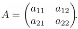
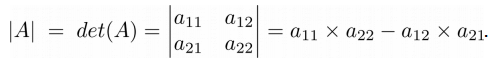
Определитель такой матрицы вычисляется следующим образом:
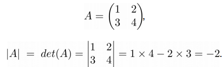
➣ Численный пример
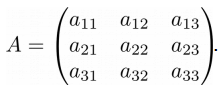
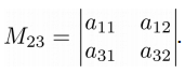
Перед тем, как привести методику расчета определителя в общем виде, введем понятие минора элемента определителя. Минор элемента определителя – это определитель, полученный из данного, путем вычеркивания всех элементов строки и столбца, на пересечении которых стоит данный элемент. Для матрицы 3×3 следующего вида:
Минор M23 будет выглядеть так:
Введем еще одно понятие – алгебраическое дополнение элемента определителя – это минор этого элемента, взятый со знаком плюс или минус:
![]()
В общем виде вычислить определитель матрицы можно через разложение определителя по элементам строки или столбца. Суть в том, что определитель равен сумме произведений элементов любой строки или столбца на их алгебраические дополнения. Для матрицы 3×3 это правило будет выполняться следующим образом:
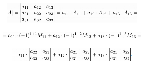
Это правило распространяется на матрицы любой размерности.
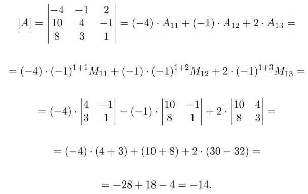
➣ Численный пример
➤ Пример на Python
На Python определитель посчитать очень просто. Создадим матрицу A размера 3×3 из приведенного выше численного примера:
>>> A = np.matrix('-4 -1 2; 10 4 -1; 8 3 1')
>>> print(A)
[[-4 -1 2]
[10 4 -1]
[ 8 3 1]]
Для вычисления определителя этой матрицы воспользуемся функцией det() из пакета linalg.
>>> np.linalg.det(A)
-14.000000000000009
Мы уже говорили про особенность работы Python с числами с плавающей точкой, поэтому можете полученное значение округлить до -14.
Свойства определителя матрицы.
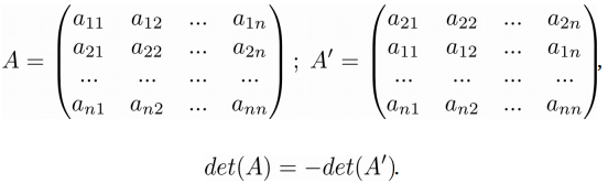
Свойство 1. Определитель матрицы остается неизменным при ее транспонировании:
![]()
➤Пример на Python
Для округления чисел будем использовать функцию round().
>>> A = np.matrix('-4 -1 2; 10 4 -1; 8 3 1')
>>> print(A)
[[-4 -1 2]
[10 4 -1]
[ 8 3 1]]
>>> print(A.T)
[[-4 10 8]
[-1 4 3]
[ 2 -1 1]]

>>> det_A = round(np.linalg.det(A), 3)
>>> det_A_t = round(np.linalg.det(A.T), 3)
>>> print(det_A)
-14.0
>>> print(det_A_t)
-14.0
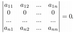
Свойство 2. Если у матрицы есть строка или столбец, состоящие из нулей, то определитель такой матрицы равен нулю:
➤ Пример на Python
>>> A = np.matrix('-4 -1 2; 0 0 0; 8 3 1')
>>> print(A)
[[-4 -1 2]
[ 0 0 0]
[ 8 3 1]]
>>> np.linalg.det(A)
0.0
Свойство 3. При перестановке строк матрицы знак ее определителя меняется на противоположный:
➤ Пример на Python
>>> A = np.matrix('-4 -1 2; 10 4 -1; 8 3 1')
>>> print(A)
[[-4 -1 2]
[10 4 -1]
[ 8 3 1]]

>>> B = np.matrix('10 4 -1; -4 -1 2; 8 3 1')
>>> print(B)
[[10 4 -1]
[-4 -1 2]
[ 8 3 1]]

>>> round(np.linalg.det(A), 3)
-14.0
>>> round(np.linalg.det(B), 3)
14.0
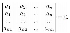
Свойство 4. Если у матрицы есть две одинаковые строки, то ее определитель равен нулю:
➤ Пример на Python
>>> A = np.matrix('-4 -1 2; -4 -1 2; 8 3 1')
>>> print(A)
[[-4 -1 2]
[-4 -1 2]
[ 8 3 1]]
>>> np.linalg.det(A)
0.0
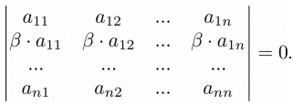
Свойство 5. Если все элементы строки или столбца матрицы умножить на какое-то число, то и определитель будет умножен на это число:

➤ Пример на Python
>>> A = np.matrix('-4 -1 2; 10 4 -1; 8 3 1')
>>> print(A)
[[-4 -1 2]
[10 4 -1]
[ 8 3 1]]

>>> k = 2
>>> B = A.copy()
>>> B[2, :] = k * B[2, :]
>>> print(B)
[[-4 -1 2]
[10 4 -1]
[16 6 2]]

>>> det_A = round(np.linalg.det(A), 3)
>>> det_B = round(np.linalg.det(B), 3)

>>> det_A * k
-28.0
>>> det_B
-28.0
Свойство 6. Если все элементы строки или столбца можно представить как сумму двух слагаемых, то определитель такой матрицы равен сумме определителей двух соответствующих матриц:

➤ Пример на Python
>>> A = np.matrix('-4 -1 2; -4 -1 2; 8 3 1')
>>> B = np.matrix('-4 -1 2; 8 3 2; 8 3 1')
>>> C = A.copy()
>>> C[1, :] += B[1, :]
>>> print(C)
[[-4 -1 2]
[ 4 2 4]
[ 8 3 1]]
>>> print(A)
[[-4 -1 2]
[-4 -1 2]
[ 8 3 1]]
>>> print(B)
[[-4 -1 2]
[ 8 3 2]
[ 8 3 1]]
>>> round(np.linalg.det(C), 3)
4.0
>>> round(np.linalg.det(A), 3) + round(np.linalg.det(B), 3)
4.0
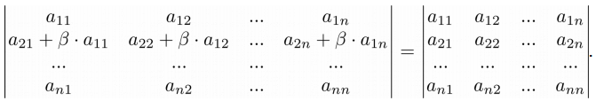
Свойство 7. Если к элементам одной строки прибавить элементы другой строки, умноженные на одно и тоже число, то определитель матрицы не изменится:
➤ Пример на Python
>>> A = np.matrix('-4 -1 2; 10 4 -1; 8 3 1')
>>> k = 2
>>> B = A.copy()
>>> B[1, :] = B[1, :] + k * B[0, :]
>>> print(A)
[[-4 -1 2]
[10 4 -1]
[ 8 3 1]]
>>> print(B)
[[-4 -1 2]
[ 2 2 3]
[ 8 3 1]]
>>> round(np.linalg.det(A), 3)
-14.0
>>> round(np.linalg.det(B), 3)
-14.0
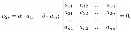
Свойство 8. Если строка или столбец матрицы является линейной комбинацией других строк (столбцов), то определитель такой матрицы равен нулю:
➤ Пример на Python
>>> A = np.matrix('-4 -1 2; 10 4 -1; 8 3 1')
>>> print(A)
[[-4 -1 2]
[10 4 -1]
[ 8 3 1]]

>>> k = 2
>>> A[1, :] = A[0, :] + k * A[2, :]
>>> round(np.linalg.det(A), 3)
0.0
Свойство 9. Если матрица содержит пропорциональные строки, то ее определитель равен нулю:
➤ Пример на Python
>>> A = np.matrix('-4 -1 2; 10 4 -1; 8 3 1')
>>> print(A)
[[-4 -1 2]
[10 4 -1]
[ 8 3 1]]
>>> k = 2
>>> A[1, :] = k * A[0, :]
>>> print(A)
[[-4 -1 2]
[-8 -2 4]
[ 8 3 1]]
>>> round(np.linalg.det(A), 3)
0.0
P.S.
Вводные уроки по “Линейной алгебре на Python” вы можете найти соответствующей странице нашего сайта. Все уроки по этой теме собраны в книге “Линейная алгебра на Python”.

Если вам интересна тема анализа данных, то мы рекомендуем ознакомиться с библиотекой Pandas. Для начала вы можете познакомиться с вводными уроками. Все уроки по библиотеке Pandas собраны в книге “Pandas. Работа с данными”.

Improve Article
Save Article
Like Article
Improve Article
Save Article
Like Article
A special number that can be calculated from a square matrix is known as the Determinant of a square matrix. The Numpy provides us the feature to calculate the determinant of a square matrix using numpy.linalg.det() function.
Syntax:
numpy.linalg.det(array)
Example 1: Calculating Determinant of a 2X2 Numpy matrix using numpy.linalg.det() function
Python3
import numpy as np
n_array = np.array([[50, 29], [30, 44]])
print("Numpy Matrix is:")
print(n_array)
det = np.linalg.det(n_array)
print("nDeterminant of given 2X2 matrix:")
print(int(det))
Output:
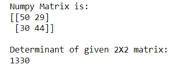
In the above example, we calculate the Determinant of the 2X2 square matrix.
Example 2: Calculating Determinant of a 3X3 Numpy matrix using numpy.linalg.det() function
Python3
import numpy as np
n_array = np.array([[55, 25, 15],
[30, 44, 2],
[11, 45, 77]])
print("Numpy Matrix is:")
print(n_array)
det = np.linalg.det(n_array)
print("nDeterminant of given 3X3 square matrix:")
print(int(det))
Output:
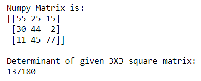
In the above example, we calculate the Determinant of the 3X3 square matrix.
Example 3: Calculating Determinant of a 5X5 Numpy matrix using numpy.linalg.det() function
Python3
import numpy as np
n_array = np.array([[5, 2, 1, 4, 6],
[9, 4, 2, 5, 2],
[11, 5, 7, 3, 9],
[5, 6, 6, 7, 2],
[7, 5, 9, 3, 3]])
print("Numpy Matrix is:")
print(n_array)
det = np.linalg.det(n_array)
print("nDeterminant of given 5X5 square matrix:")
print(int(det))
Output:
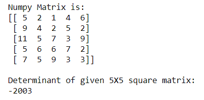
In the above example, we calculate the Determinant of the 5X5 square matrix.
Last Updated :
05 Sep, 2020
Like Article
Save Article
Find the code for this post on GitHub.
![]()
Why This Post?
Like the previous post, once we decide to wean ourselves off numpy and scipy, NOT because we don’t love them (we do love them) or want to use them (we do want to use them), but mostly so that we can learn machine learning principles more deeply by understanding how to code the tools ourselves, all of those basic helper functions from the post on basic tools also become necessary. AND, understanding the math to coding steps for determinants IS actually slightly, if not VERY, helpful and insightful.
Furthermore, a new data science expert acquaintance of mine, that I had the pleasure of hearing speak recently, stated something in his talk that stayed with me (and I paraphrase), “I continue to study linear algebra to gain more insights into machine learning and AI.” Such ongoing effort is very much the spirit of this blog.
Math Background
I am a big fan of studying multiple references when learning, or reviewing, something important to me, so I don’t mind telling you that I reviewed the wiki page for determinants, and I personally felt that it is quite good. However, while this is going to look a bit like that page, I will be injecting my own personal slants on determinant steps with a view to the upcoming coding of those steps and will be constructively lazy. Also, as a starting “linear algebraish” note, this is for SQUARE matrices.
Let’s start with a 2 x 2 matrix.
A=begin{bmatrix} a_{11} & a_{12} \ a_{21} & a_{22} end{bmatrix}
vert A vert = a_{11} cdot a_{22} — a_{21} cdot a_{12}
Equations 1: A 2 x 2 Matrix A and the Method to Calculate It’s Determinant
What’s is the above saying? For any 2 x 2 matrix, the determinant is a scalar value equal to the product of the main diagonal elements minus the product of it’s counter diagonal elements.
I really wish that all size matrices could be calculated this easily. The post would be trivial at best if it was. And yet, in essence, the whole method does boil down to this basic operation AFTER you see how to get to this step many times over for larger and larger matrices. The steps that break the calculation of a determinant down to this point aren’t hard either. They’re actually quite simple, BUT they are NOT easy!
If I were you, what I am about to show you, IF you’ve never seen it before, would scare my lazy self! However, PLEASE stay courageous in your endeavors to stay constructively lazy, because you will, I hope, be amazed at how few lines of code we need to break down into the steps required to calculate a determinant for any size matrix. However, there is an even better, more efficient, and faster way to find a determinant with some exceptional constructive laziness! I will be showing the math to code for both methods, AND we’ve essentially done most of the work for the second method in two previous recent blog posts.
So, walking before we run, how would one find the determinant of a 3 x 3 matrix using the first (classical) method?
A=begin{bmatrix} a_{11} & a_{12} & a_{13} \ a_{21} & a_{22} & a_{23} \ a_{31} & a_{32} & a_{33} end{bmatrix}
vert A vert = begin{vmatrix} a_{11} & a_{12} & a_{13} \ a_{21} & a_{22} & a_{23} \ a_{31} & a_{32} & a_{33} end{vmatrix} = a_{11} begin{vmatrix} square & square & square \ square & a_{22} & a_{23} \ square & a_{32} & a_{33} end{vmatrix} -a_{12} begin{vmatrix} square & square & square \ a_{21} & square & a_{23} \ a_{31} & square & a_{33} end{vmatrix} + a_{13} begin{vmatrix} square & square & square \ a_{21} & a_{22} & square \ a_{31} & a_{32} & square end{vmatrix}
= a_{11} begin{vmatrix}a_{22} & a_{23} \ a_{32} & a_{33} end{vmatrix} -a_{12} begin{vmatrix}a_{21} & a_{23} \ a_{31} & a_{33} end{vmatrix} + a_{13} begin{vmatrix}a_{21} & a_{22} \ a_{31} & a_{32} end{vmatrix}
vert A vert = a_{11} cdot lparen a_{22} cdot a_{33} — a_{32} cdot a_{23} rparen -a_{12} cdot lparen a_{21} cdot a_{33} — a_{31} cdot a_{23} rparen + a_{13} cdot lparen a_{21} cdot a_{32} — a_{31} cdot a_{22} rparen
Equations 2: A 3 x 3 Matrix A and the Methods to Calculate It’s Determinant
That was a bit intimidating, and it gets worse for larger and larger matrices. If you mostly work with 3 x 3 matrices, you really want to know how to use the rule of Sarrus also, because it’s really simple to remember, and to calculate by hand, and to code if you want to. However, for those brave souls that came here to learn to do the real work of calculating a determinant for ANY size matrix, the rule of Sarrus is only a stepping stone to one location – the determinants for 3×3 matrices.
Points to note from Equations 2:
- Start with the first row, and use those elements as multipliers, WITH ALTERNATING SIGNS, on the SUB 2 x 2 matrices as shown.
- The 2 x 2 matrices are formed by NOT using the row and column that the multiplier from step 1 is in.
I almost hate to point this out, but let’s be thorough here. You could also do, in essence, the same approach by starting with the first column instead of the first row:
- Start with the first column, and use those elements as multipliers, WITH ALTERNATING SIGNS, on the SUB 2 x 2 matrices.
- The 2 x 2 matrices are formed by NOT using the row and column that the multiplier from step 1 is in.
You tough guys and gals who are more stoic and less constructively lazy than us mere mortal math people may be thinking, “Dang, Thom! You’re such a wimp!” While that’s true, maybe seeing the next step AND imagining going to larger and larger size matrices will cause you to cringe in mathematical laziness a bit more!
A=begin{bmatrix} a_{11} & a_{12} & a_{13} & a_{14} \ a_{21} & a_{22} & a_{23} & a_{24} \ a_{31} & a_{32} & a_{33} & a_{34} \ a_{41} & a_{42} & a_{43} & a_{44} end{bmatrix}
vert A vert = begin{vmatrix} a_{11} & a_{12} & a_{13} & a_{14} \ a_{21} & a_{22} & a_{23} & a_{24} \ a_{31} & a_{32} & a_{33} & a_{34} \ a_{41} & a_{42} & a_{43} & a_{44} end{vmatrix} = a_{11} begin{vmatrix} square & square & square & square \ square & a_{22} & a_{23} & a_{24} \ square & a_{32} & a_{33} & a_{34} \ square & a_{42} & a_{43} & a_{44} end{vmatrix} -a_{12} begin{vmatrix} square & square & square & square \ a_{21} & square & a_{23} & a_{24} \ a_{31} & square & a_{33} & a_{34} \ a_{41} & square & a_{43} & a_{44} end{vmatrix}
+ a_{13} begin{vmatrix} square & square & square & square \ a_{21} & a_{22} & square & a_{24} \ a_{31} & a_{32} & square & a_{34} \ a_{41} & a_{42} & square & a_{44} end{vmatrix} — a_{14} begin{vmatrix} square & square & square & square \ a_{21} & a_{22} & a_{23} & square \ a_{31} & a_{32} & a_{33} & square \ a_{41} & a_{42} & a_{43} & square end{vmatrix}
Equations 3: A 4 x 4 Matrix A and the PART of the Methods to Calculate It’s Determinant.
EACH Submatrix HERE Must Be Calculated from Equations 2!
The one reason that I love the above is that it STRONGLY reminds me WHY I LOVE coding and symbolic math solvers! So, as the caption above says, the steps shown in Equations 3 merely help us get to the point where we can do the steps in Equations 2 for each submatrix of Equations 3, AND, as you’ve likely realized, Equations 2 actually include the steps of Equations 1 for each submatrix. Phew! I trust you to imagine what we’d do for n x n matrices where n > 4. Again, simple enough, but NOT easy!
The Code
Thanks to the power of recursive function calls (a function that cleverly calls itself at the right steps), we can code this method for any size square matrix in as few as 14 lines with a call to one additional function that is only 6 lines of code (white space and comments not included). Our recursive function is below. The repo version of this code is in LinearAlgebraPurePython.py. In that version, the function has MORE documentation and it’s formatted a bit differently.
def determinant_recursive(A, total=0):
    # Section 1: store indices in list for row referencing
    indices = list(range(len(A)))

    # Section 2: when at 2x2 submatrices recursive calls end
    if len(A) == 2 and len(A[0]) == 2:
        val = A[0][0] * A[1][1] - A[1][0] * A[0][1]
        return val

    # Section 3: define submatrix for focus column and
    #      call this function
    for fc in indices: # A) for each focus column, ...
        # find the submatrix ...
        As = copy_matrix(A) # B) make a copy, and ...
        As = As[1:] # ... C) remove the first row
        height = len(As) # D)

        for i in range(height):
            # E) for each remaining row of submatrix ...
            #     remove the focus column elements
            As[i] = As[i][0:fc] + As[i][fc+1:]

        sign = (-1) ** (fc % 2) # F)
        # G) pass submatrix recursively
        sub_det = determinant_recursive(As)
        # H) total all returns from recursion
        total += sign * A[0][fc] * sub_det

    return total
Let’s go through the code sections by number:
- Store the indices for the matrix that’s passed in. This is a handy trick that we learned in a previous post, but we’ll show how it’s handy below.
- If the incoming matrix is a 2 x 2 matrix, calculate and return it’s determinant. This is one bite of the meat of the method!
- This section handles the remaining meat of the method, minus the one bite in 2. We begin with a) a for loop for each focus column. Next, b) we make a copy of the A matrix and call it As for the current A_{submatrix}. Why the copy? We do NOT want to confuse As and A, because they are different, and we need to use A in this same function scope. Next, to get As in the correct form, c) we eliminate the first row, and then, creating the d) height parameter for readability (this was NOT absolutely necessary), we enter a nested for loop to e) remove the fc elements in each row as explained in the equations discussion of the math background section above. f) We then use our handy one line method to get the right alternation of signs (by using +1 or -1) for the sign of our submatrix multiplier. Next, g) we call this function with our new submatrix as the A matrix! If you’re at a point in your programming where recursion still causes you to feel faint, I think we can all be sympathetic to that. Hang in there. Your intuition with recursive calls will blossom. Think about the recursion this way – each call will keep coming to this point with a new submatrix, BUT when the submatrix is a 2 , x , 2, it will finally return a number for the recursive branch that it’s on, which our miraculous coding language and computer are handling, and h) sum those up into our total variable correctly. Once all branches have been depleted, the totaling will be complete, and the completed total will be returned to the top level call. Phew!
But wait Thom! You never explained the total = 0 default parameter in the initial call. I CONFESS – MORE LAZINESS! It could have been the first line of code actually, but I was just trying to save a line of code. Try it both ways. It works. As always, refactor to your liking.
Now for testing. In the repo is a function that imports our LinearAlgebraPurePython.py module and numpy for checking this code (YES, my laziness DOES extend to using numpy as a gold standard check) and it’s called BasicToolsPractice.py. The lines applicable to our work in this post so far and the results applicable to these lines of code are shown below in the next two code blocks, respectively. Sorry if the 5×5 A matrix wraps on your screen.
import LinearAlgebraPurePython as la
import numpy as np


A = [[-2,2,-3],[-1,1,3],[2,0,-1]] # Matrix from wiki
Det = la.determinant_recursive(A)
npDet = np.linalg.det(A)
print("Determinant of A is", round(Det,9))
print("The Numpy Determinant of A is", round(npDet,9))
print()

A = [[1,2,3,4],[5,6,7,8],[9,10,11,12],[13,14,15,16]]
Det = la.determinant_recursive(A)
npDet = np.linalg.det(A)
print("Determinant of A is", Det)
print("The Numpy Determinant of A is", npDet)
print()

A = [[1,2,3,4],[8,5,6,7],[9,12,10,11],[13,14,16,15]]
Det = la.determinant_recursive(A)
npDet = np.linalg.det(A)
print("Determinant of A is", Det)
print("The Numpy Determinant of A is", round(npDet,9))
print()

A = [[1,2,3,4,1],[8,5,6,7,2],[9,12,10,11,3],[13,14,16,15,4],[10,8,6,4,2]]
Det = la.determinant_recursive(A)
npDet = np.linalg.det(A)
print("Determinant of A is", Det)
print("The Numpy Determinant of A is", round(npDet,9))
print()
The next code block is output from the above:
Determinant of A is 18
The Numpy Determinant of A is 18.0

Determinant of A is 0
The Numpy Determinant of A is 0.0

Determinant of A is -348
The Numpy Determinant of A is -348.0

Determinant of A is -240
The Numpy Determinant of A is -240.0
A More Efficient Way
You programmers that are into Big O thinking are cringing right now, and you should be! Yes, this gets expensive for ginormous matrices. There’s a much faster way for bigger matrices like I promised above. Please refer to my post on matrix inversion or solving a system of equations if you have not yet done so. To avoid offending Google and to help my early rankings to date, I wish to avoid repeating much of that material here. You needn’t read both posts; just read one. Or don’t. See if you first understand it from the little bit of math and code below and from the determinant wiki.
The More Efficient Math
PLEASE DON’T BE MAD AT ME! Why did I take us thru all that stuff above? One of many reasons was that showing the method above, besides possibly causing some of you recursive programming trauma, which is a right of programming passage, was to help you appreciate this method more! I can’t imagine that it didn’t work!
A = begin{bmatrix} a_{11} & a_{12} & a_{13} & a_{14} \ a_{21} & a_{22} & a_{23} & a_{24} \ a_{31} & a_{32} & a_{33} & a_{34} \ a_{41} & a_{42} & a_{43} & a_{44} end{bmatrix}, ,,,,, A_{M} = begin{bmatrix} am_{11} & am_{12} & am_{13} & am_{14} \ 0 & am_{22} & am_{23} & am_{24} \ 0 & 0 & am_{33} & am_{34} \ 0 & 0 & 0 & am_{44} end{bmatrix}
vert A_{M} vert = am_{11} cdot am_{22} cdot am_{33} cdot am_{44}
Equations 4: Matrix Determinant Method of First Creating an Upper Triangle Matrix thru Row Operations
and then Calculating the Product of the Main Diagonal
If we do row operations to put A (truly any size A) into upper triangle form, we need only calculate the product of the elements of the main diagonal to get the determinant. Geeks be excited!
(Geek is a positive term in my vocabulary – be a Geek and be proud).
Oh OH! In your technical textbooks, when the author would point out an important point and say that, “The proof is left as an exercise for the student?” MAN, DID I HATE THAT!!!
(Attempting to sound like a technical textbook author now) “If you start with an upper triangle matrix and apply the first method that we covered previously, you will find that the determinant does in fact reduce to the product of the elements on the main diagonal.”
I confess that it’s much more fun to write that than to read. LAZY – I agree.
If you visit the matrix inversion post or the solving a system of equations post, and then compare the math steps code below to the code from one of those posts, you’ll see how we’ve combined and simplified the steps, but I’ll still explain them here.
Steps to Reduce Any Square Matrix to an Upper Triangle Matrix
We’ll move from left to right on the matrix columns, and each column will have an element from the main diagonal in it, of course, which we’ll call fd:
- For each row below the row with fd in it, we create a scaler that is equal to (element in row that is in the same column as fd) divided by (fd).
- We update each row below the row with fd in it with (current row) – scaler * (row with fd in it).
- This will drive the elements in each row below fd to 0.
- When we advance to the next fd, we only need to repeat these steps for the rows below the row with the current fd in it.
Once the matrix is in upper triangle form, the determinant is simply the product of all elements on the main diagonal.
Is that easy to code? I hope that you think so. Here’s the code. Again, the documentation of the function in the module in the repo is more complete and formatted a little differently.
def determinant_fast(A):
    # Section 1: Establish n parameter and copy A
    n = len(A)
    AM = copy_matrix(A)

    # Section 2: Row ops on A to get in upper triangle form
    for fd in range(n): # A) fd stands for focus diagonal
        for i in range(fd+1,n): # B) only use rows below fd row
            if AM[fd][fd] == 0: # C) if diagonal is zero ...
                AM[fd][fd] == 1.0e-18 # change to ~zero
            # D) cr stands for "current row"
            crScaler = AM[i][fd] / AM[fd][fd]
            # E) cr - crScaler * fdRow, one element at a time
            for j in range(n):
                AM[i][j] = AM[i][j] - crScaler * AM[fd][j]

    # Section 3: Once AM is in upper triangle form ...
    product = 1.0
    for i in range(n):
        # ... product of diagonals is determinant
        product *= AM[i][i]

    return product
No way! Yes. Let’s go through the numbered sections:
- We make a copy of A and call it A_M to preserve A.
- a) Cycle thru the columns from left to right using the outer most for loop, which is really controlling the focus diagonal (fd) that we want to use. b) Only cycle through the rows below the row with fd in it. c) If the diagonal element is zero, make it very VERY small instead. CHEATER! Yes, I am cheating BIG TIME! And I am PROUD OF IT! This is a very good constructively LAZY cheat. (I did develop a fancy way to reorder rows based on the number of leading zeros and keep track of how many times that was done, so that I could change the final sign of the determinant, but DANG! Just more code and more steps. Cheating was better! If you’re not sure what I am talking about, read the determinant wiki again near the bottom of the “Properties of the determinant” section. d) Create your scaler for each row as described previously, and then e) perform the row operation to drive the element of the current row that is below fd to 0.
- With the A_M matrix in upper triangle form, the determinant is the product of the elements on the main diagonal. Then, simply return that product.
Now, let’s put this new determinant function into practice. Again, I am showing the applicable lines from the BasicToolsPractice.py file in the repo.
import LinearAlgebraPurePython as la
import numpy as np


A = [[-2,2,-3],[-1,1,3],[2,0,-1]] # Matrix from wiki
Det = la.determinant_fast(A)
npDet = np.linalg.det(A)
print("Determinant of A is", round(Det,9))
print("The Numpy Determinant of A is", round(npDet,9))
print()

A = [[1,2,3,4],[5,6,7,8],[9,10,11,12],[13,14,15,16]]
Det = la.determinant_fast(A)
npDet = np.linalg.det(A)
print("Determinant of A is", round(Det,9)+0)
print("The Numpy Determinant of A is", round(npDet,9))
print()

A = [[1,2,3,4],[8,5,6,7],[9,12,10,11],[13,14,16,15]]
Det = la.determinant_fast(A)
npDet = np.linalg.det(A)
print("Determinant of A is", round(Det,9))
print("The Numpy Determinant of A is", round(npDet,9))
print()

A = [[1,2,3,4,1],[8,5,6,7,2],[9,12,10,11,3],[13,14,16,15,4],[10,8,6,4,2]]
Det = la.determinant_fast(A)
npDet = np.linalg.det(A)
print("Determinant of A is", round(Det,9))
print("The Numpy Determinant of A is", round(npDet,9))
print()
And the results for those lines are …
Determinant of A is 18.0
The Numpy Determinant of A is 18.0

Determinant of A is 0.0
The Numpy Determinant of A is 0.0

Determinant of A is -348.0
The Numpy Determinant of A is -348.0

Determinant of A is -240.0
The Numpy Determinant of A is -240.0
Closing
With this post in place, and with all the previous posts (chronologically speaking that is and minus the MAD post), we finally have the tool set that we need to perform a Least Squares regression, which will be the next post.
I really hope that you found some useful insights from this post. I believe the upcoming posts will begin to show the spirit of what we want to gain, insights wise, from this blog. And as always, please clone, refactor, and make the code your own! Until the next post …
- linalg.det(a)[source]#
-
Compute the determinant of an array.
- Parameters:
-
- a(…, M, M) array_like
-
Input array to compute determinants for.
- Returns:
-
- det(…) array_like
-
Determinant of a.
See also
slogdet-
Another way to represent the determinant, more suitable for large matrices where underflow/overflow may occur.
scipy.linalg.det-
Similar function in SciPy.
Notes
New in version 1.8.0.
Broadcasting rules apply, see the
numpy.linalgdocumentation for
details.The determinant is computed via LU factorization using the LAPACK
routinez/dgetrf.Examples
The determinant of a 2-D array [[a, b], [c, d]] is ad — bc:
>>> a = np.array([[1, 2], [3, 4]])
>>> np.linalg.det(a)
-2.0 # may vary
Computing determinants for a stack of matrices:
>>> a = np.array([ [[1, 2], [3, 4]], [[1, 2], [2, 1]], [[1, 3], [3, 1]] ])
>>> a.shape
(3, 2, 2)
>>> np.linalg.det(a)
array([-2., -3., -8.])
I’ve used as base idea of Peyman Naseri and want to share with my implementation,
import numpy as np
import time

def minor(arr,i,j):
    c = arr[:]
    c = np.delete(c, (i),axis=0)
    return [np.delete(row, (j),axis=0) for row in (c)]


def det(arr):
    n = len(arr)
    if n == 1 :return arr[0][0]
    if n == 2 :return arr[0][0]*arr[1][1] - arr[0][1]*arr[1][0]
    sum = 0
    for i in range(0,n):
        m = minor(arr,0,i)
        sum =sum + ((-1)**i)*arr[0][i] * det(m)
    return sum

matrix = np.random.randint(-5, 5, size=(10, 10)) # martix nxn with integer values in interval [-5, 5)

print(matrix)
start_time = time.time()
print("started:", start_time)
det(matrix)
end_time = time.time()
print("finished:", end_time)
print("--- %s seconds ---" % (end_time - start_time))
as result determinant calculation for matrix 10*10 on my laptop takes about 1 minute, I understand that my code not optimal but main reason for this implementation (maybe I lost something) I just need to get working code base on Peyman Naseri solution which seems to me very pretty.
[[ 2 -1 -1  0 -2  0  4  4  3  4]
 [-3  1 -1  3  0 -3 -2  0  3 -1]
 [ 2 -1 -4  3  0 -2 -2 -5  3 -5]
 [-2 -1  2 -2  4 -3 -5 -1 -5  3]
 [ 1 -4  1 -5 -5  4 -3 -5  3  1]
 [ 2  4  0 -1 -1 -5 -2 -2 -3 -5]
 [ 1  4 -3 -4 -5  0  0  0 -5 -1]
 [ 0 -5 -5  4 -3 -2  2 -4  2 -5]
 [-3  1 -1 -4  4 -5  3 -3 -4  0]
 [ 0 -2  2 -3  1  3  2  0 -1  4]]
started: 1636896388.0213237
finished: 1636896442.846928
--- 54.82560420036316 seconds ---