Как найти дисперсию произведения случайных величин - Исправление недочетов и поиск решений вместе с Examum.ru

В заметке рассмотрены основные свойства математического ожидания и дисперсии с доказательствами.

В статье приняты следующие обозначения:

(a ) — неслучайная величина (константа)

(X, Y ) — случайные величины

(M[X]) — Математическое ожидание X

(D[X]) — Дисперсия X

Математическое ожидание

Математическое ожидание неслучайной величины

[ M[a] = a]

Доказательство:

Доказать, это достаточно очевидное, свойство можно, рассматривая неслучайную величину как частный вид случайной, при одном возможном значении с вероятностью единица; тогда по общей формуле для математического ожидания:

[ M[a] = a * 1 = a ]

Математическое ожидание линейно

[ M[aX + bY] = aM[X] + bM[Y]]

Доказательство вынесения неслучайной величины за знак математического ожидания

[ M[aX] = a M[X] ]

Доказательство прямо следует из линейности суммы и интеграла.

Следует специально отметить, что теорема сложения математических ожиданий справедлива для любых случайных величин — как зависимых, так и независимых.

Теорема сложения математических ожиданий обобщается на произвольное число слагаемых.

Для дискретных величин

[ M[aX] = sum_{i} a x_i p _i = a sum_{i} x_i p_i = a M[X]]

Для непрерывных величин

[ M[aX] = intop_{ infty }^{infty} a x f(x) dx = a intop_{ infty }^{infty} x f(x) dx = a M[X]]

Доказательство математического ожидания суммы случайных величин

а) Пусть ((X, Y) ) — система дискретных случайных величин. Применим к сумме случайных величин общую формулу для математического ожидания функции двух аргументов:

[ M[X + Y] = sum_{i} sum_{j} (x_i + y_i) p_{ij} \
= sum_{i}sum_{j} x_i p_{ij} + sum_{i}sum_{j} y_i p_{ij} \
= sum_{i} x_isum_{j} p_{ij} + sum_{j} y_jsum_{i} p_{ij} ]

Но (sum_{j} p_{ij} ) представляет собой не что иное, как полную вероятность того, что величина (X ) примет значение (x_i ):

[ sum_{j} p_{ij} = P(X = x_i) = p_i ]

следовательно,

[ sum_{i} x_isum_{j} p_{ij} = sum_{i} x_i p_i = M[X] ]

Аналогично докажем, что

[ sum_{j} y_jsum_{i} p_{ij} = M[Y] ]

б) Пусть ((X, Y) ) — система непрерывных случайных величин.

[ M[X + Y] = int intop_{ infty }^{infty } (x+y) f(x,y) dx dy = int intop_{ infty }^{infty } x f(x,y) dx dy + int intop_{ infty }^{infty } y f(x,y) dx dy ]

Преобразуем первый из интегралов:

[ int intop_{ infty }^{infty } x f(x,y) dx dy = intop_{ infty }^{infty } x (intop_{ infty }^{infty } f(x,y)dy) dx = intop_{ infty }^{infty } x f_1(x) dx = M[X] ]

аналогично второй:

[ int intop_{ infty }^{infty } y f(x,y) dx dy = M[X] ]

Математическое ожидание произведения

Математическое ожидание произведения двух случайных величин равно произведению их математических ожиданий плюс корреляционный момент:

[ M[XY] = M[X] M[Y] + cov(XY)]

для независимых величин:

[ M[XY] = M[X] M[Y] ]

Доказательство

Будем исходить из определения корреляционного момента:

[ cov(X,Y) = M[ stackrel{ circ }{X} stackrel{ circ }{Y} ] = M[(X- M[X])(Y-M[Y])] ]

Преобразуем это выражение, пользуясь свойствами математического ожидания:

[ cov(X,Y) = M[(X- M[X])(Y-M[Y])] = \
M[XY] — M[X] M[Y] — M[Y]M[X] + M[X]M[Y] = \
M[X Y] — M[X] M[Y] ]

что, очевидно, равносильно доказываемому соотношению

Дисперсия

Дисперсия случайной величины есть характеристика рассеивания, разбросанности значений случайной величины около её математического ожидания.

[ D[X] = M[X^2] — (M[X])^2 ]

Дисперсия не зависит от знака

[ D[-X] = D[X] ]

Дисперсия суммы случайной и постоянной величин

[ D[X+b] = D[X] ]

Дисперсия неслучайной величины

[ D[a] = 0 ]

Доказательство:

По определению дисперсии:

[ D[a] = M[stackrel{ circ }{a^2}] = M[a — M[a]^2 ] = M[(a-a)^2] = M[0] = 0]

Дисперсия суммы случайных величин

[ D[X+Y] = D[X] + D[Y] + 2*cov(X,Y) ]

Доказательство:

Обозначим (XY = Z ).

По теореме сложения математических ожиданий:

[ M[Z] = M[X] + M[Y] ]

Перейдем от случайных величин (X, Y, Z ). к соответствующим центрированным величинам (stackrel{ circ }{X}, stackrel{ circ }{Y}, stackrel{ circ }{Z} ), имеем:

[ stackrel{ circ }{Z} = stackrel{ circ }{X} + stackrel{ circ }{Y} ]

По определению дисперсии

[ D[X+Y] = D[Z] = M[stackrel{ circ }{Z}^2] = M[stackrel{ circ }{X}^2] + 2M[stackrel{ circ }{X} stackrel{ circ }{Y}] + M[stackrel{ circ }{Y}^2] \
= D[X] + 2 cov(X,Y) + D[Y] ]

Дисперсия произведения неслучайной величины на случайную

[ D[aX] = a^2 D[X]]

Доказательство:

По определению дисперсии

[ D[aX] = M[(a X — M[a X])^2] = M[(a X — a M[X])^2] = a^2 M[(X — M[X])^2] = c^2 D[X] ]

Дисперсия произведения независимых величин

[ D[XY] = D[X] D[Y] + (M[X])^2 D[Y] + (M[Y])^2 D[X]]

Доказательство:

Обозначим (XY = Z ). По определению дисперсии

[ D[XY] = D[Z] = M[Z^2] = M[Z-M[Z]]^2]

Так как величины (XY) независимы, то (M[Z] = M[X]M[Y]) и

[ D[XY] = M[(XY — M[X]M[Y])^2] \

= M[X^2 Y^2] — 2M[X]M[Y]M[XY]+ M[X]^2M[Y]^2 ]

При независимых (XY) величины (X^2Y^2) также независимы, следовательно:

[ M[X^2 Y^2] = M[X^2] M[Y^2], M[XY] = M[X]M[Y]]

[ D[XY] = M[X^2]M[Y^2] — M[X]^2M[Y]^2 ]

но (M[X]^2) есть не что иное, как второй начальный момент величины (X) , и, следовательно, выражается через дисперсию:

[ M[X^2] = D[X]+M[X]^2 ]

аналогично

[ M[Y^2] = D[Y]+M[Y]^2 ]

Подставляя эти выражения и приводя подобные члены, приходим к формуле

[ D[XY] = D[X] D[Y] + (M[X])^2 D[Y] + (M[Y])^2 D[X]]

Источник

A product distribution is a probability distribution constructed as the distribution of the product of random variables having two other known distributions. Given two statistically independent random variables X and Y, the distribution of the random variable Z that is formed as the product Z=XY is a product distribution.

Algebra of random variables[edit]

The product is one type of algebra for random variables: Related to the product distribution are the ratio distribution, sum distribution (see List of convolutions of probability distributions) and difference distribution. More generally, one may talk of combinations of sums, differences, products and ratios.

Many of these distributions are described in Melvin D. Springer’s book from 1979 The Algebra of Random Variables.^[1]

Derivation for independent random variables[edit]

If and are two independent, continuous random variables, described by probability density functions $f_{X}$ and $f_{Y}$ then the probability density function of Z=XY is^[2]

${displaystyle f_{Z}(z)=int _{-infty }^{infty }f_{X}(x)f_{Y}(z/x){frac {1}{|x|}},dx.}$

Proof[edit]

We first write the cumulative distribution function of starting with its definition

${displaystyle {begin{aligned}F_{Z}(z)&,{stackrel {text{def}}{=}} mathbb {P} (Zleq z)\&=mathbb {P} (XYleq z)\&=mathbb {P} (XYleq z,Xgeq 0)+mathbb {P} (XYleq z,Xleq 0)\&=mathbb {P} (Yleq z/X,Xgeq 0)+mathbb {P} (Ygeq z/X,Xleq 0)\&=int _{0}^{infty }f_{X}(x)int _{-infty }^{z/x}f_{Y}(y),dy,dx+int _{-infty }^{0}f_{X}(x)int _{z/x}^{infty }f_{Y}(y),dy,dxend{aligned}}}$

We find the desired probability density function by taking the derivative of both sides with respect to . Since on the right hand side, appears only in the integration limits, the derivative is easily performed using the fundamental theorem of calculus and the chain rule. (Note the negative sign that is needed when the variable occurs in the lower limit of the integration.)

${displaystyle {begin{aligned}f_{Z}(z)&=int _{0}^{infty }f_{X}(x)f_{Y}(z/x){frac {1}{x}},dx-int _{-infty }^{0}f_{X}(x)f_{Y}(z/x){frac {1}{x}},dx\&=int _{0}^{infty }f_{X}(x)f_{Y}(z/x){frac {1}{|x|}},dx+int _{-infty }^{0}f_{X}(x)f_{Y}(z/x){frac {1}{|x|}},dx\&=int _{-infty }^{infty }f_{X}(x)f_{Y}(z/x){frac {1}{|x|}},dx.end{aligned}}}$

where the absolute value is used to conveniently combine the two terms.^[3]

Alternate proof[edit]

A faster more compact proof begins with the same step of writing the cumulative distribution of starting with its definition:

${displaystyle {begin{aligned}F_{Z}(z)&{overset {underset {mathrm {def} }{}}{=}} mathbb {P} (Zleq z)\&=mathbb {P} (XYleq z)\&=int _{-infty }^{infty }int _{-infty }^{infty }f_{X}(x)f_{Y}(y)u(z-xy),dy,dxend{aligned}}}$

where is the Heaviside step function and serves to limit the region of integration to values of and satisfying .

We find the desired probability density function by taking the derivative of both sides with respect to .

${displaystyle {begin{aligned}f_{Z}(z)&=int _{-infty }^{infty }int _{-infty }^{infty }f_{X}(x)f_{Y}(y)delta (z-xy),dy,dx\&=int _{-infty }^{infty }f_{X}(x)f_{Y}(z/x)left[int _{-infty }^{infty }delta (z-xy),dyright],dx\&=int _{-infty }^{infty }f_{X}(x)f_{Y}(z/x){frac {1}{|x|}},dx.end{aligned}}}$

where we utilize the translation and scaling properties of the Dirac delta function delta .

A more intuitive description of the procedure is illustrated in the figure below. The joint pdf ${displaystyle f_{X}(x)f_{Y}(y)}$ exists in the — plane and an arc of constant value is shown as the shaded line. To find the marginal probability ${displaystyle f_{Z}(z)}$ on this arc, integrate over increments of area on this contour.

Diagram to illustrate the product distribution of two variables.

Starting with ${displaystyle y={frac {z}{x}}}$ , we have ${displaystyle dy=-{frac {z}{x^{2}}},dx=-{frac {y}{x}},dx}$ . So the probability increment is ${displaystyle delta p=f(x,y),dx,|dy|=f_{X}(x)f_{Y}(z/x){frac {y}{|x|}},dx,dx}$ . Since implies , we can relate the probability increment to the -increment, namely ${displaystyle delta p=f_{X}(x)f_{Y}(z/x){frac {1}{|x|}},dx,dz}$ . Then integration over , yields ${displaystyle f_{Z}(z)=int f_{X}(x)f_{Y}(z/x){frac {1}{|x|}},dx}$ .

A Bayesian interpretation[edit]

Let be a random sample drawn from probability distribution ${displaystyle f_{x}(x)}$ . Scaling by theta generates a sample from scaled distribution ${displaystyle theta Xsim {frac {1}{|theta |}}f_{X}left({frac {x}{theta }}right)}$ which can be written as a conditional distribution ${displaystyle g_{x}(x|theta )={frac {1}{|theta |}}f_{x}left({frac {x}{theta }}right)}$ .

Letting theta be a random variable with pdf ${displaystyle f_{theta }(theta )}$ , the distribution of the scaled sample becomes ${displaystyle f_{X}(theta x)=g_{X}(xmid theta )f_{theta }(theta )}$ and integrating out theta we get ${displaystyle h_{x}(x)=int _{-infty }^{infty }g_{X}(x|theta )f_{theta }(theta )dtheta }$ so is drawn from this distribution ${displaystyle theta Xsim h_{X}(x)}$ . However, substituting the definition of we also have
${displaystyle h_{X}(x)=int _{-infty }^{infty }{frac {1}{|theta |}}f_{x}left({frac {x}{theta }}right)f_{theta }(theta ),dtheta }$ which has the same form as the product distribution above. Thus the Bayesian posterior distribution ${displaystyle h_{X}(x)}$ is the distribution of the product of the two independent random samples theta and .

For the case of one variable being discrete, let theta have probability $P_{i}$ at levels ${displaystyle theta _{i}}$ with ${displaystyle sum _{i}P_{i}=1}$ . The conditional density is ${displaystyle f_{X}(xmid theta _{i})={frac {1}{|theta _{i}|}}f_{x}left({frac {x}{theta _{i}}}right)}$ . Therefore ${displaystyle f_{X}(theta x)=sum {frac {P_{i}}{|theta _{i}|}}f_{X}left({frac {x}{theta _{i}}}right)}$ .

Expectation of product of random variables[edit]

When two random variables are statistically independent, the expectation of their product is the product of their expectations. This can be proved from the law of total expectation:

{displaystyle operatorname {E} (XY)=operatorname {E} (operatorname {E} (XYmid Y))}

In the inner expression, Y is a constant. Hence:

{displaystyle operatorname {E} (XYmid Y)=Ycdot operatorname {E} [Xmid Y]}

{displaystyle operatorname {E} (XY)=operatorname {E} (Ycdot operatorname {E} [Xmid Y])}

This is true even if X and Y are statistically dependent in which case is a function of Y. In the special case in which X and Y are statistically
independent, it is a constant independent of Y. Hence:

{displaystyle operatorname {E} (XY)=operatorname {E} (Ycdot operatorname {E} [X])}

{displaystyle operatorname {E} (XY)=operatorname {E} (X)cdot operatorname {E} (Y)}

Variance of the product of independent random variables[edit]

Let X,Y be uncorrelated random variables with means ${displaystyle mu _{X},mu _{Y},}$ and variances ${displaystyle sigma _{X}^{2},sigma _{Y}^{2}}$ .
If, additionally, the random variables $X^{2}$ and Y^2 are uncorrelated, then the variance of the product XY is

${displaystyle operatorname {Var} (XY)=(sigma _{X}^{2}+mu _{X}^{2})(sigma _{Y}^{2}+mu _{Y}^{2})-mu _{X}^{2}mu _{Y}^{2}}$

In the case of the product of more than two variables, if ${displaystyle X_{1}cdots X_{n},;;n>2}$ are statistically independent then^[4] the variance of their product is

${displaystyle operatorname {Var} (X_{1}X_{2}cdots X_{n})=prod _{i=1}^{n}(sigma _{i}^{2}+mu _{i}^{2})-prod _{i=1}^{n}mu _{i}^{2}}$

Characteristic function of product of random variables[edit]

Assume X, Y are independent random variables. The characteristic function of X is $varphi _{X}(t)$ , and the distribution of Y is known. Then from the law of total expectation, we have^[5]

${displaystyle {begin{aligned}varphi _{Z}(t)&=operatorname {E} (e^{itXY})\&=operatorname {E} (operatorname {E} (e^{itXY}mid Y))\&=operatorname {E} (varphi _{X}(tY))end{aligned}}}$

If the characteristic functions and distributions of both X and Y are known, then alternatively, ${displaystyle varphi _{Z}(t)=operatorname {E} (varphi _{Y}(tX))}$ also holds.

Mellin transform[edit]

The Mellin transform of a distribution f(x) with support only on xgeq 0 and having a random sample is

${displaystyle {mathcal {M}}f(x)=varphi (s)=int _{0}^{infty }x^{s-1}f(x),dx=operatorname {E} [X^{s-1}].}$

The inverse transform is

${displaystyle {mathcal {M}}^{-1}varphi (s)=f(x)={frac {1}{2pi i}}int _{c-iinfty }^{c+iinfty }x^{-s}varphi (s),ds.}$

if are two independent random samples from different distributions, then the Mellin transform of their product is equal to the product of their Mellin transforms:

$mathcal{M}_{XY}(s) = mathcal{M}_X(s)mathcal{M}_Y(s)$

If s is restricted to integer values, a simpler result is

${displaystyle operatorname {E} [(XY)^{n}]=operatorname {E} [X^{n}];operatorname {E} [Y^{n}]}$

Thus the moments of the random product are the product of the corresponding moments of and this extends to non-integer moments, for example

${displaystyle operatorname {E} [{(XY)^{1/p}}]=operatorname {E} [X^{1/p}];operatorname {E} [Y^{1/p}].}$

The pdf of a function can be reconstructed from its moments using the saddlepoint approximation method.

A further result is that for independent X, Y

${displaystyle operatorname {E} [X^{p}Y^{q}]=operatorname {E} [X^{p}]operatorname {E} [Y^{q}]}$

Gamma distribution example To illustrate how the product of moments yields a much simpler result than finding the moments of the distribution of the product, let X,Y be sampled from two Gamma distributions, ${displaystyle f_{Gamma}(x;theta ,1)=Gamma (theta )^{-1}x^{theta -1}e^{-x}}$ with parameters
whose moments are

${displaystyle operatorname {E} [X^{p}]=int _{0}^{infty }x^{p}Gamma (x,theta ),dx={frac {Gamma (theta +p)}{Gamma (theta )}}.}$

Multiplying the corresponding moments gives the Mellin transform result

${displaystyle operatorname {E} [(XY)^{p}]=operatorname {E} [X^{p}];operatorname {E} [Y^{p}]={frac {Gamma (alpha +p)}{Gamma (alpha )}};{frac {Gamma (beta +p)}{Gamma (beta )}}}$

Independently, it is known that the product of two independent Gamma-distributed samples (~Gamma(α,1) and Gamma(β,1)) has a K-distribution:

${displaystyle f(z,alpha ,beta )=2Gamma (alpha )^{-1}Gamma (beta )^{-1}z^{{frac {alpha +beta }{2}}-1}K_{alpha -beta }(2{sqrt {z}})={frac {1}{alpha beta }}f_{K}left({frac {z}{alpha beta }};1,alpha ,beta right),;zgeq 0}$

To find the moments of this, make the change of variable , simplifying similar integrals to:

${displaystyle int _{0}^{infty }z^{p}K_{nu }(2{sqrt {z}}),dz=2^{-2p-1}int _{0}^{infty }y^{2p+1}K_{nu }(y),dy}$

thus

${displaystyle 2int _{0}^{infty }z^{{frac {alpha +beta }{2}}-1}K_{alpha -beta }(2{sqrt {z}}),dz=2^{-(alpha +beta )-2p+1}int _{0}^{infty }y^{(alpha +beta )+2p-1}K_{alpha -beta }(y),dy}$

The definite integral

${displaystyle int _{0}^{infty }y^{mu }K_{nu }(y),dy=2^{mu -1}Gamma left({frac {1+mu +nu }{2}}right)Gamma left({frac {1+mu -nu }{2}}right)}$

is well documented and we have finally

${displaystyle {begin{aligned}E[Z^{p}]&={frac {2^{-(alpha +beta )-2p+1};2^{(alpha +beta )+2p-1}}{Gamma (alpha );Gamma (beta )}}Gamma left({frac {(alpha +beta +2p)+(alpha -beta )}{2}}right)Gamma left({frac {(alpha +beta +2p)-(alpha -beta )}{2}}right)\\&={frac {Gamma (alpha +p),Gamma (beta +p)}{Gamma (alpha ),Gamma (beta )}}end{aligned}}}$

which, after some difficulty, has agreed with the moment product result above.

If X, Y are drawn independently from Gamma distributions with shape parameters then

${displaystyle operatorname {E} [X^{p}Y^{q}]=operatorname {E} [X^{p}];operatorname {E} [Y^{q}]={frac {Gamma (alpha +p)}{Gamma (alpha )}};{frac {Gamma (beta +q)}{Gamma (beta )}}}$

This type of result is universally true, since for bivariate independent variables ${displaystyle f_{X,Y}(x,y)=f_{X}(x)f_{Y}(y)}$ thus

${displaystyle {begin{aligned}operatorname {E} [X^{p}Y^{q}]&=int _{x=-infty }^{infty }int _{y=-infty }^{infty }x^{p}y^{q}f_{X,Y}(x,y),dy,dx\&=int _{x=-infty }^{infty }x^{p}{Big [}int _{y=-infty }^{infty }y^{q}f_{Y}(y),dy{Big ]}f_{X}(x),dx\&=int _{x=-infty }^{infty }x^{p}f_{X}(x),dxint _{y=-infty }^{infty }y^{q}f_{Y}(y),dy\&=operatorname {E} [X^{p}];operatorname {E} [Y^{q}]end{aligned}}}$

or equivalently it is clear that ${displaystyle X^{p}{text{ and }}Y^{q}}$ are independent variables.

Special cases[edit]

Lognormal distributions[edit]

The distribution of the product of two random variables which have lognormal distributions is again lognormal. This is itself a special case of a more general set of results where the logarithm of the product can be written as the sum of the logarithms. Thus, in cases where a simple result can be found in the list of convolutions of probability distributions, where the distributions to be convolved are those of the logarithms of the components of the product, the result might be transformed to provide the distribution of the product. However this approach is only useful where the logarithms of the components of the product are in some standard families of distributions.

Uniformly distributed independent random variables[edit]

Let be the product of two independent variables ${displaystyle Z=X_{1}X_{2}}$ each uniformly distributed on the interval [0,1], possibly the outcome of a copula transformation. As noted in «Lognormal Distributions» above, PDF convolution operations in the Log domain correspond to the product of sample values in the original domain. Thus, making the transformation , such that ${displaystyle p_{U}(u),|du|=p_{X}(x),|dx|}$ , each variate is distributed independently on u as

${displaystyle p_{U}(u)={frac {p_{X}(x)}{|du/dx|}}={frac {1}{x^{-1}}}=e^{u},;;-infty <uleq 0}$

and the convolution of the two distributions is the autoconvolution

${displaystyle c(y)=int _{u=0}^{y}e^{u}e^{y-u}du=-int _{u=y}^{0}e^{y}du=-ye^{y},;;-infty <yleq 0}$

Next retransform the variable to ${displaystyle z=e^{y}}$ yielding the distribution

${displaystyle c_{2}(z)=c_{Y}(y)/|dz/dy|={frac {-ye^{y}}{e^{y}}}=-y=ln(1/z)}$

on the interval [0,1]

For the product of multiple (> 2) independent samples the characteristic function route is favorable. If we define then above is a Gamma distribution of shape 1 and scale factor 1, ${displaystyle c({tilde {y}})={tilde {y}}e^{-{tilde {y}}}}$ , and its known CF is ${displaystyle (1-it)^{-1}}$ . Note that so the Jacobian of the transformation is unity.

The convolution of independent samples from therefore has CF ${displaystyle (1-it)^{-n}}$ which is known to be the CF of a Gamma distribution of shape :

${displaystyle c_{n}({tilde {y}})=Gamma (n)^{-1}{tilde {y}}^{(n-1)}e^{-{tilde {y}}}=Gamma (n)^{-1}(-y)^{(n-1)}e^{y}}$

Making the inverse transformation ${displaystyle z=e^{y}}$ we get the PDF of the product of the n samples:

${displaystyle f_{n}(z)={frac {c_{n}(y)}{|dz/dy|}}=Gamma (n)^{-1}{Big (}-log z{Big )}^{n-1}e^{y}/e^{y}={frac {{Big (}-log z{Big )}^{n-1}}{(n-1)!;;;}};;;0<zleq 1}$

The following, more conventional, derivation from Stackexchange^[6] is consistent with this result.
First of all, letting ${displaystyle Z_{2}=X_{1}X_{2}}$ its CDF is

${displaystyle {begin{aligned}F_{Z_{2}}(z)=Pr {Big [}Z_{2}leq z{Big ]}&=int _{x=0}^{1}Pr {Big [}X_{2}leq {frac {z}{x}}{Big ]}f_{X_{1}}(x),dx\&=int _{x=0}^{z}1dx+int _{x=z}^{1}{frac {z}{x}},dx\&=z-zlog z,;;0<zleq 1end{aligned}}}$

The density of ${displaystyle z_{2}{text{ is then }}f(z_{2})=-log(z_{2})}$

Multiplying by a third independent sample gives distribution function

${displaystyle {begin{aligned}F_{Z_{3}}(z)=Pr {Big [}Z_{3}leq z{Big ]}&=int _{x=0}^{1}Pr {Big [}X_{3}leq {frac {z}{x}}{Big ]}f_{Z_{2}}(x),dx\&=-int _{x=0}^{z}log(x),dx-int _{x=z}^{1}{frac {z}{x}}log(x),dx\&=-z{Big (}log(z)-1{Big )}+{frac {1}{2}}zlog ^{2}(z)end{aligned}}}$

Taking the derivative yields
${displaystyle f_{Z_{3}}(z)={frac {1}{2}}log ^{2}(z),;;0<zleq 1.}$

The author of the note conjectures that, in general,
${displaystyle f_{Z_{n}}(z)={frac {(-log z)^{n-1}}{(n-1)!;;;}},;;0<zleq 1}$

The geometry of the product distribution of two random variables in the unit square.

The figure illustrates the nature of the integrals above. The shaded area within the unit square and below the line z = xy, represents the CDF of z. This divides into two parts. The first is for 0 < x < z where the increment of area in the vertical slot is just equal to dx. The second part lies below the xy line, has y-height z/x, and incremental area dx z/x.

Independent central-normal distributions[edit]

The product of two independent Normal samples follows a modified Bessel function. Let x, y be samples from a Normal(0,1) distribution and .
Then

${displaystyle p_{Z}(z)={frac {K_{0}(|z|)}{pi }},;;;-infty <z<+infty }$

The variance of this distribution could be determined, in principle, by a definite integral from Gradsheyn and Ryzhik,^[7]

${displaystyle int _{0}^{infty }x^{mu }K_{nu }(ax),dx=2^{mu -1}a^{-mu -1}Gamma {Big (}{frac {1+mu +nu }{2}}{Big )}Gamma {Big (}{frac {1+mu -nu }{2}}{Big )},;;a>0,;nu +1pm mu >0}$

thus
${displaystyle int _{-infty }^{infty }{frac {z^{2}K_{0}(|z|)}{pi }},dz={frac {4}{pi }};Gamma ^{2}{Big (}{frac {3}{2}}{Big )}=1}$

A much simpler result, stated in a section above, is that the variance of the product of zero-mean independent samples is equal to the product of their variances. Since the variance of each Normal sample is one, the variance of the product is also one.

[edit]

The product of correlated Normal samples case was recently addressed by Nadarajaha and Pogány.^[8]
Let be zero mean, unit variance, normally distributed variates with correlation coefficient

Then

${displaystyle f_{Z}(z)={frac {1}{pi {sqrt {1-rho ^{2}}}}}exp left({frac {rho z}{1-rho ^{2}}}right)K_{0}left({frac {|z|}{1-rho ^{2}}}right)}$

Mean and variance: For the mean we have from the definition of correlation coefficient. The variance can be found by transforming from two unit variance zero mean uncorrelated variables U, V. Let

${displaystyle X=U,;;Y=rho U+{sqrt {(1-rho ^{2})}}V}$

Then X, Y are unit variance variables with correlation coefficient rho and

${displaystyle (XY)^{2}=U^{2}{bigg (}rho U+{sqrt {(1-rho ^{2})}}V{bigg )}^{2}=U^{2}{bigg (}rho ^{2}U^{2}+2rho {sqrt {1-rho ^{2}}}UV+(1-rho ^{2})V^{2}{bigg )}}$

Removing odd-power terms, whose expectations are obviously zero, we get

${displaystyle operatorname {E} [(XY)^{2}]=rho ^{2}operatorname {E} [U^{4}]+(1-rho ^{2})operatorname {E} [U^{2}]operatorname {E} [V^{2}]=3rho ^{2}+(1-rho ^{2})=1+2rho ^{2}}$

Since ${displaystyle (operatorname {E} [Z])^{2}=rho ^{2}}$ we have

${displaystyle operatorname {Var} (Z)=operatorname {E} [Z^{2}]-(operatorname {E} [Z])^{2}=1+2rho ^{2}-rho ^{2}=1+rho ^{2}}$

High correlation asymptote
In the highly correlated case, the product converges on the square of one sample. In this case the ${displaystyle K_{0}}$ asymptote is ${displaystyle K_{0}(x)rightarrow {sqrt {tfrac {pi }{2x}}}e^{-x}{text{ in the limit as }}x={frac {|z|}{1-rho ^{2}}}rightarrow infty }$
and

${displaystyle {begin{aligned}p(z)&rightarrow {frac {1}{pi {sqrt {1-rho ^{2}}}}}exp left({frac {rho z}{1-rho ^{2}}}right){sqrt {frac {pi (1-rho ^{2})}{2z}}}exp left(-{frac {|z|}{1-rho ^{2}}}right)\&={frac {1}{sqrt {2pi z}}}exp {Bigg (}{frac {-|z|+rho z}{(1-rho )(1+rho )}}{Bigg )}\&={frac {1}{sqrt {2pi z}}}exp {Bigg (}{frac {-z}{1+rho }}{Bigg )},;;z>0\&rightarrow {frac {1}{Gamma ({tfrac {1}{2}}){sqrt {2z}}}}e^{-{tfrac {z}{2}}},;;{text{ as }}rho rightarrow 1\end{aligned}}}$

which is a Chi-squared distribution with one degree of freedom.

Multiple correlated samples. Nadarajaha et al. further show that if ${displaystyle Z_{1},Z_{2},..Z_{n}{text{ are }}n}$ iid random variables sampled from ${displaystyle f_{Z}(z)}$ and ${displaystyle {bar {Z}}={tfrac {1}{n}}sum Z_{i}}$ is their mean then

${displaystyle f_{bar {Z}}(z)={frac {n^{n/2}2^{-n/2}}{Gamma ({frac {n}{2}})}}|z|^{n/2-1}exp left({frac {beta -gamma }{2}}zright){W}_{0,{frac {1-n}{2}}}(|z|),;;-infty <z<infty .}$

where W is the Whittaker function while ${displaystyle beta ={frac {n}{1-rho }},;;gamma ={frac {n}{1+rho }}}$ .

Using the identity ${displaystyle W_{0,nu }(x)={sqrt {frac {x}{pi }}}K_{nu }(x/2),;;xgeq 0}$ , see for example the DLMF compilation. eqn(13.13.9),^[9] this expression can be somewhat simplified to

${displaystyle f_{bar {z}}(z)={frac {n^{n/2}2^{-n/2}}{Gamma ({frac {n}{2}})}}|z|^{n/2-1}exp left({frac {beta -gamma }{2}}zright){sqrt {{frac {beta +gamma }{pi }}|z|}};K_{frac {1-n}{2}}left({frac {beta +gamma }{2}}|z|right),;;-infty <z<infty .}$

The pdf gives the distribution of a sample covariance. The approximate distribution of a correlation coefficient can be found via the Fisher transformation.

Multiple non-central correlated samples. The distribution of the product of correlated non-central normal samples was derived by Cui et al.^[10] and takes the form of an infinite series of modified Bessel functions of the first kind.

Moments of product of correlated central normal samples

For a central normal distribution N(0,1) the moments are

${displaystyle operatorname {E} [X^{p}]={frac {1}{sigma {sqrt {2pi }}}}int _{-infty }^{infty }x^{p}exp(-{tfrac {x^{2}}{2sigma ^{2}}}),dx={begin{cases}0&{text{if }}p{text{ is odd,}}\sigma ^{p}(p-1)!!&{text{if }}p{text{ is even.}}end{cases}}}$

where n!! denotes the double factorial.

If are central correlated variables, the simplest bivariate case of the multivariate normal moment problem described by Kan,^[11] then

${displaystyle operatorname {E} [X^{p}Y^{q}]={begin{cases}0&{text{if }}p+q{text{ is odd,}}\{frac {p!q!}{2^{tfrac {p+q}{2}}}}sum _{k=0}^{t}{frac {(2rho )^{2k}}{{Big (}{frac {p}{2}}-k{Big )}!;{Big (}{frac {q}{2}}-k{Big )}!;(2k)!}}&{text{if }}p{text{ and }}q{text{ are even}}\{frac {p!q!}{2^{tfrac {p+q}{2}}}}sum _{k=0}^{t}{frac {(2rho )^{2k+1}}{{Big (}{frac {p-1}{2}}-k{Big )}!;{Big (}{frac {q-1}{2}}-k{Big )}!;(2k+1)!}}&{text{if }}p{text{ and }}q{text{ are odd}}end{cases}}}$

where

is the correlation coefficient and

[needs checking]

[edit]

The distribution of the product of non-central correlated normal samples was derived by Cui et al.^[10] and takes the form of an infinite series.

These product distributions are somewhat comparable to the Wishart distribution. The latter is the joint distribution of the four elements (actually only three independent elements) of a sample covariance matrix. If ${displaystyle x_{t},y_{t}}$ are samples from a bivariate time series then the ${displaystyle W=sum _{t=1}^{K}{dbinom {x_{t}}{y_{t}}}{dbinom {x_{t}}{y_{t}}}^{T}}$ is a Wishart matrix with K degrees of freedom. The product distributions above are the unconditional distribution of the aggregate of K > 1 samples of ${displaystyle W_{2,1}}$ .

Independent complex-valued central-normal distributions[edit]

Let ${displaystyle u_{1},v_{1},u_{2},v_{2}}$ be independent samples from a normal(0,1) distribution.
Setting
${displaystyle z_{1}=u_{1}+iv_{1}{text{ and }}z_{2}=u_{2}+iv_{2}{text{ then }}z_{1},z_{2}}$ are independent zero-mean complex normal samples with circular symmetry. Their complex variances are ${displaystyle operatorname {Var} |z_{i}|=2.}$

The density functions of

${displaystyle r_{i}equiv |z_{i}|=(u_{i}^{2}+v_{i}^{2})^{frac {1}{2}},;;i=1,2}$

are Rayleigh distributions defined as:

${displaystyle f_{r}(r_{i})=r_{i}e^{-r_{i}^{2}/2}{text{ of mean }}{sqrt {tfrac {pi }{2}}}{text{ and variance}}{frac {4-pi }{2}}}$

The variable ${displaystyle y_{i}equiv r_{i}^{2}}$ is clearly Chi-squared with two degrees of freedom and has PDF

${displaystyle f_{y_{i}}(y_{i})={tfrac {1}{2}}e^{-y_{i}/2}{text{ of mean value }}2}$

Wells et al.^[12] show that the density function of ${displaystyle sequiv |z_{1}z_{2}|}$ is

${displaystyle f_{s}(s)=sK_{0}(s),;;sgeq 0}$

and the cumulative distribution function of is

${displaystyle P(a)=Pr[sleq a]=int _{s=0}^{a}sK_{0}(s)ds=1-aK_{1}(a)}$

Thus the polar representation of the product of two uncorrelated complex Gaussian samples is

${displaystyle f_{s,theta }(s,theta )=f_{s}(s)p_{theta }(theta ){text{ where }}p(theta ){text{ is uniform on }}[0,2pi ]}$

The first and second moments of this distribution can be found from the integral in Normal Distributions above

${displaystyle m_{1}=int _{0}^{infty }s^{2}K_{0}(s),dx=2Gamma ^{2}({tfrac {3}{2}})=2({tfrac {sqrt {pi }}{2}})^{2}={frac {pi }{2}}}$

${displaystyle m_{2}=int _{0}^{infty }s^{3}K_{0}(s),dx=2^{2}Gamma ^{2}({tfrac {4}{2}})=4}$

Thus its variance is ${displaystyle operatorname {Var} (s)=m_{2}-m_{1}^{2}=4-{frac {pi ^{2}}{4}}}$ .

Further, the density of ${displaystyle zequiv s^{2}={|r_{1}r_{2}|}^{2}={|r_{1}|}^{2}{|r_{2}|}^{2}=y_{1}y_{2}}$ corresponds to the product of two independent Chi-square samples $y_{i}$ each with two DoF. Writing these as scaled Gamma distributions ${displaystyle f_{y}(y_{i})={tfrac {1}{theta Gamma (1)}}e^{-y_{i}/theta }{text{ with }}theta =2}$ then, from the Gamma products below, the density of the product is

${displaystyle f_{Z}(z)={tfrac {1}{2}}K_{0}({sqrt {z}}){text{ with expectation }}operatorname {E} (z)=4}$

Independent complex-valued noncentral normal distributions[edit]

The product of non-central independent complex Gaussians is described by O’Donoughue and Moura^[13] and forms a double infinite series of modified Bessel functions of the first and second types.

Gamma distributions[edit]

The product of two independent Gamma samples, ${displaystyle z=x_{1}x_{2}}$ , defining ${displaystyle Gamma (x;k_{i},theta _{i})={frac {x^{k_{i}-1}e^{-x/theta _{i}}}{Gamma (k_{i})theta _{i}^{k_{i}}}}}$ , follows^[14]

${displaystyle {begin{aligned}p_{Z}(z)&={frac {2}{Gamma (k_{1})Gamma (k_{2})}}{frac {z^{{frac {k_{1}+k_{2}}{2}}-1}}{(theta _{1}theta _{2})^{frac {k_{1}+k_{2}}{2}}}}K_{k_{1}-k_{2}}left(2{sqrt {frac {z}{theta _{1}theta _{2}}}}right)\\&={frac {2}{Gamma (k_{1})Gamma (k_{2})}}{frac {y^{{frac {k_{1}+k_{2}}{2}}-1}}{theta _{1}theta _{2}}}K_{k_{1}-k_{2}}left(2{sqrt {y}}right){text{ where }}y={frac {z}{theta _{1}theta _{2}}}\end{aligned}}}$

Beta distributions[edit]

Nagar et al.^[15] define a correlated bivariate beta distribution

${displaystyle f(x,y)={frac {x^{a-1}y^{b-1}(1-x)^{b+c-1}(1-y)^{a+c-1}}{B(a,b,c)(1-xy)^{a+b+c}}},;;;0<x,y<1}$

where

${displaystyle B(a,b,c)={frac {Gamma (a)Gamma (b)Gamma (c)}{Gamma (a+b+c)}}}$

Then the pdf of Z = XY is given by

${displaystyle f_{Z}(z)={frac {B(a+c,b+c)z^{a-1}(1-z)^{c-1}}{B(a,b,c)}}{_{2}F_{1}}(a+c,a+c;a+b+2c;1-z),;;;0<z<1}$

where ${displaystyle {_{2}F_{1}}}$ is the Gauss hypergeometric function defined by the Euler integral

${displaystyle {_{2}F_{1}}(a,b,c,z)={frac {Gamma (c)}{Gamma (a)Gamma (c-a)}}int _{0}^{1}v^{a-1}(1-v)^{c-a-1}(1-vz)^{-b},dv}$

Note that multivariate distributions are not generally unique, apart from the Gaussian case, and there may be alternatives.

Uniform and gamma distributions[edit]

The distribution of the product of a random variable having a uniform distribution on (0,1) with a random variable having a gamma distribution with shape parameter equal to 2, is an exponential distribution.^[16] A more general case of this concerns the distribution of the product of a random variable having a beta distribution with a random variable having a gamma distribution: for some cases where the parameters of the two component distributions are related in a certain way, the result is again a gamma distribution but with a changed shape parameter.^[16]

The K-distribution is an example of a non-standard distribution that can be defined as a product distribution (where both components have a gamma distribution).

Gamma and Pareto distributions[edit]

The product of n Gamma and m Pareto independent samples was derived by Nadarajah.^[17]

Notes[edit]

^ Springer, Melvin Dale (1979). The Algebra of Random Variables. Wiley. ISBN 978-0-471-01406-5. Retrieved 24 September 2012.
^ Rohatgi, V. K. (1976). An Introduction to Probability Theory and Mathematical Statistics. Wiley Series in Probability and Statistics. New York: Wiley. doi:10.1002/9781118165676. ISBN 978-0-19-853185-2.
^ Grimmett, G. R.; Stirzaker, D.R. (2001). Probability and Random Processes. Oxford: Oxford University Press. ISBN 978-0-19-857222-0. Retrieved 4 October 2015.
^ Sarwate, Dilip (March 9, 2013). «Variance of product of multiple random variables». Stack Exchange.
^ «How to find characteristic function of product of random variables». Stack Exchange. January 3, 2013.
^ heropup (1 February 2014). «product distribution of two uniform distribution, what about 3 or more». Stack Exchange.
^ Gradsheyn, I S; Ryzhik, I M (1980). Tables of Integrals, Series and Products. Academic Press. pp. section 6.561.
^ Nadarajah, Saralees; Pogány, Tibor (2015). «On the distribution of the product of correlated normal random variables». Comptes Rendus de l’Académie des Sciences, Série I. 354 (2): 201–204. doi:10.1016/j.crma.2015.10.019.
^ Equ(13.18.9). «Digital Library of Mathematical Functions». NIST: National Institute of Standards and Technology.
^ ^a ^b Cui, Guolong (2016). «Exact Distribution for the Product of Two Correlated Gaussian Random Variables». IEEE Signal Processing Letters. 23 (11): 1662–1666. Bibcode:2016ISPL…23.1662C. doi:10.1109/LSP.2016.2614539.
^ Kan, Raymond (2008). «From moments of sum to moments of product». Journal of Multivariate Analysis. 99 (3): 542–554. doi:10.1016/j.jmva.2007.01.013.
^ Wells, R T; Anderson, R L; Cell, J W (1962). «The Distribution of the Product of Two Central or Non-Central Chi-Square Variates». The Annals of Mathematical Statistics. 33 (3): 1016–1020. doi:10.1214/aoms/1177704469.
^ O’Donoughue, N; Moura, J M F (March 2012). «On the Product of Independent Complex Gaussians». IEEE Transactions on Signal Processing. 60 (3): 1050–1063. Bibcode:2012ITSP…60.1050O. doi:10.1109/TSP.2011.2177264.
^ Wolfies (August 2017). «PDF of the product of two independent Gamma random variables». stackexchange.
^ Nagar, D K; Orozco-Castañeda, J M; Gupta, A K (2009). «Product and quotient of correlated beta variables». Applied Mathematics Letters. 22: 105–109. doi:10.1016/j.aml.2008.02.014.
^ ^a ^b
Johnson, Norman L.; Kotz, Samuel; Balakrishnan, N. (1995). Continuous Univariate Distributions Volume 2, Second edition. Wiley. p. 306. ISBN 978-0-471-58494-0. Retrieved 24 September 2012.
^ Nadarajah, Saralees (June 2011). «Exact distribution of the product of n gamma and m Pareto random variables». Journal of Computational and Applied Mathematics. 235 (15): 4496–4512. doi:10.1016/j.cam.2011.04.018.

References[edit]

Springer, Melvin Dale; Thompson, W. E. (1970). «The distribution of products of beta, gamma and Gaussian random variables». SIAM Journal on Applied Mathematics. 18 (4): 721–737. doi:10.1137/0118065. JSTOR 2099424.
Springer, Melvin Dale; Thompson, W. E. (1966). «The distribution of products of independent random variables». SIAM Journal on Applied Mathematics. 14 (3): 511–526. doi:10.1137/0114046. JSTOR 2946226.

Источник

Функции случайных величин

Определение функции случайных величин. Функция дискретного случайного аргумента и ее числовые характеристики. Функция непрерывного случайного аргумента и ее числовые характеристики. Функции двух случайных аргументов. Определение функции распределения вероятностей и плотности для функции двух случайных аргументов.

Закон распределения вероятностей функции одной случайной величины

При решении задач, связанных с оценкой точности работы различных автоматических систем, точности производства отдельных элементов систем и др., часто приходится рассматривать функции одной или нескольких случайных величин. Такие функции также являются случайными величинами. Поэтому при решении задач необходимо знать законы распределения фигурирующих в задаче случайных величин. При этом обычно известны закон распределения системы случайных аргументов и функциональная зависимость.

Таким образом, возникает задача, которую можно сформулировать так.

Дана система случайных величин (X_1,X_2,ldots,X_n) , закон распределения которой известен. Рассматривается некоторая случайная величина Y как функция данных случайных величин:

Y=varphi(X_1,X_2,ldots,X_n).

(6.1)

Требуется определить закон распределения случайной величины , зная вид функций (6.1) и закон совместного распределения ее аргументов.

Рассмотрим задачу о законе распределения функции одного случайного аргумента

Y=varphi(X).

Пусть — дискретная случайная величина, имеющая ряд распределения

$begin{array}{|c|c|c|c|c|}hline{X}&x_1&x_2&cdots&x_n\hline{P}&p_1&p_2&cdots&p_n\hlineend{array}$

Тогда Y=varphi(X) также дискретная случайная величина с возможными значениями y_1=varphi(x_1),y_2=varphi(x_2),ldots,y_n=varphi(x_n) . Если все значения y_1,y_2,ldots,y_n различны, то для каждого k=1,2,ldots,n события ${X=x_k}$ и ${Y=y_k=varphi(x_k)}$ тождественны. Следовательно,

$P{Y=y_k}=P{X=x_k}=p_k$

и искомый ряд распределения имеет вид

$begin{array}{|c|c|c|c|c|}hline{Y}&y_1=varphi(x_1)&y_2=varphi(x_2)&cdots&y_n=varphi(x_n)\hline{P}&p_1&p_2&cdots&p_n\hlineend{array}$

Если же среди чисел y_1=varphi(x_1),y_2=varphi(x_2),ldots,y_n=varphi(x_n) есть одинаковые, то каждой группе одинаковых значений y_k=varphi(x_k) нужно отвести в таблице один столбец и соответствующие вероятности сложить.

Для непрерывных случайных величин задача ставится так: зная плотность распределения f(x) случайной величины , найти плотность распределения g(y) случайной величины Y=varphi(X) . При решении поставленной задачи рассмотрим два случая.

Предположим сначала, что функция y=varphi(x) является монотонно возрастающей, непрерывной и дифференцируемой на интервале (a;b) , на котором лежат все возможные значения величины . Тогда обратная функция x=psi(y) существует, при этом являясь также монотонно возрастающей, непрерывной и дифференцируемой. В этом случае получаем

g(y)=fbigl(psi(y)bigr)cdot |psi'(y)|.

(6.2)

Пример 1. Случайная величина распределена с плотностью

$f(x)=frac{1}{sqrt{2pi}}e^{-x^2/2}$

Найти закон распределения случайной величины , связанной с величиной зависимостью Y=X^3 .

Решение. Так как функция y=x^3 монотонна на промежутке (-infty;+infty) , то можно применить формулу (6.2). Обратная функция по отношению к функции varphi(x)=x^3 есть psi(y)=sqrt[LARGE{LARGE{3}}]{y} , ее производная $psi'(y)=frac{1}{3sqrt[LARGE{LARGE{3}}]{y^2}}$ . Следовательно,

$g(y)=frac{1}{3sqrt{2pi}}e^{-sqrt[LARGE{LARGE{3}}]{y^2}/2}frac{1}{sqrt[LARGE{LARGE{3}}]{y^2}}$

Рассмотрим случай немонотонной функции. Пусть функция y=varphi(x) такова, что обратная функция x=psi(y) неоднозначна, т. е. одному значению величины соответствует несколько значений аргумента , которые обозначим x_1=psi_1(y),x_2=psi_2(y),ldots,x_n=psi_n(y) , где — число участков, на которых функция y=varphi(x) изменяется монотонно. Тогда

$g(y)=sumlimits_{k=1}^{n}fbigl(psi_k(y)bigr)cdot |psi'_k(y)|.$

(6.3)

Пример 2. В условиях примера 1 найти распределение случайной величины Y=X^2 .

Решение. Обратная функция x=psi(y) неоднозначна. Одному значению аргумента соответствуют два значения функции

$begin{gathered}x_1=psi_1(y)=+sqrt{y};\x_2=psi_2(y)=-sqrt{y}.end{gathered}$

Применяя формулу (6.3), получаем:

$begin{gathered}g(y)=f(psi_1(y))|psi'_1(y)|+f(psi_2(y))|psi'_2(y)|=\\=frac{1}{sqrt{2pi}},e^{-left(-sqrt{y^2}right)^2/2}!left|-frac{1}{2sqrt{y}}right|+frac{1}{sqrt{2pi}},e^{-left(sqrt{y^2}right)^2/2}!left|frac{1}{2sqrt{y}}right|=frac{1}{sqrt{2pi{y}}},e^{-y/2}.end{gathered}$

Закон распределения функции двух случайных величин

Пусть случайная величина является функцией двух случайных величин, образующих систему (X_1;X_2) , т. е. Y=varphi(X_1;X_2) . Задача состоит в том, чтобы по известному распределению системы найти распределение случайной величины .

Пусть f(x_1;x_2) — плотность распределения системы случайных величин . Введем в рассмотрение новую величину Y_1 , равную X_1 , и рассмотрим систему уравнений

$left{!begin{gathered}y=varphi(x_1;x_2);hfill\y_1=x_1.hfillend{gathered}right.$

Будем полагать, что эта система однозначно разрешима относительно x_1,x_2

$left{!begin{gathered}x_2=psi(y;y_2);hfill\x_1=y_1.hfillend{gathered}right.$

и удовлетворяет условиям дифференцируемости.

Плотность распределения случайной величины

$g_1(y)=intlimits_{-infty}^{+infty}f(x_1;psi(y;x_1))!left|frac{partialpsi(y;x_1)}{partial{y}}right|dx_1.$

Заметим, что рассуждения не изменяются, если введенную новую величину Y_1 положить равной X_2 .

Математическое ожидание функции случайных величин

На практике часто встречаются случаи, когда нет особой надобности полностью определять закон распределения функции случайных величин, а достаточно только указать его числовые характеристики. Таким образом, возникает задача определения числовых характеристик функций случайных величин помимо законов распределения этих функций.

Пусть случайная величина является функцией случайного аргумента с заданным законом распределения

Y=varphi(X).

Требуется, не находя закона распределения величины , определить ее математическое ожидание

M(Y)=M[varphi(X)].

Пусть — дискретная случайная величина, имеющая ряд распределения

$begin{array}{|c|c|c|c|c|}hline{x_i}&x_1&x_2&cdots&x_n\hline{p_i}&p_1&p_2&cdots&p_n\hlineend{array}$

Составим таблицу значений величины и вероятностей этих значений:

$begin{array}{|c|c|c|c|c|}hline{y_i=varphi(x_i)}&y_1=varphi(x_1)&y_2=varphi(x_2)&cdots&y_n=varphi(x_n)\hline{p_i}&p_1&p_2&cdots&p_n\hlineend{array}$

Эта таблица не является рядом распределения случайной величины , так как в общем случае некоторые из значений могут совпадать между собой и значения в верхней строке не обязательно идут в возрастающем порядке. Однако математическое ожидание случайной величины можно определить по формуле

$M[varphi(X)]=sumlimits_{i=1}^{n}varphi(x_i)p_i,$

(6.4)

так как величина, определяемая формулой (6.4), не может измениться от того, что под знаком суммы некоторые члены будут заранее объединены, а порядок членов изменен.

Формула (6.4) не содержит в явном виде закон распределения самой функции varphi(X) , а содержит только закон распределения аргумента . Таким образом, для определения математического ожидания функции Y=varphi(X) вовсе не требуется знать закон распределения функции , а достаточно знать закон распределения аргумента .

Для непрерывной случайной величины математическое ожидание вычисляется по формуле

$M[varphi(X)]=intlimits_{-infty}^{+infty}varphi(x)f(x),dx,$

где f(x) — плотность распределения вероятностей случайной величины .

Рассмотрим случаи, когда для нахождения математического ожидания функции случайных аргументов не требуется знание даже законов распределения аргументов, а достаточно знать только некоторые их числовые характеристики. Сформулируем эти случаи в виде теорем.

Теорема 6.1. Математическое ожидание суммы как зависимых, так и независимых двух случайных величин равно сумме математических ожиданий этих величин:

M(X+Y)=M(X)+M(Y).

Теорема 6.2. Математическое ожидание произведения двух случайных величин равно произведению их математических ожиданий плюс корреляционный момент:

$M(XY)=M(X)M(Y)+mu_{xy}.$

Следствие 6.1. Математическое ожидание произведения двух некоррелированных случайных величин равно произведению их математических ожиданий.

Следствие 6.2. Математическое ожидание произведения двух независимых случайных величин равно произведению их математических ожиданий.

Дисперсия функции случайных величин

По определению дисперсии имеем D[Y]=M[(Y-M(Y))^2]. . Следовательно,

D[varphi(x)]=M[(varphi(x)-M(varphi(x)))^2] , где M(varphi(x))=M[varphi(X)] .

Приведем расчетные формулы только для случая непрерывных случайных аргументов. Для функции одного случайного аргумента Y=varphi(X) дисперсия выражается формулой

$D[varphi(x)]=intlimits_{-infty}^{+infty}(varphi(x)-M(varphi(x)))^2f(x),dx,$

(6.5)

где M(varphi(x))=M[varphi(X)] — математическое ожидание функции ; f(x) — плотность распределения величины .

Формулу (6.5) можно заменить на следующую:

$D[varphi(x)]=intlimits_{-infty}^{+infty}varphi^2(x)f(x),dx-M^2(X)$

Рассмотрим теоремы о дисперсиях, которые играют важную роль в теории вероятностей и ее приложениях.

Теорема 6.3. Дисперсия суммы случайных величин равна сумме дисперсий этих величин плюс удвоенная сумма корреляционных моментов каждой из слагаемых величин со всеми последующими:

$D!left[sumlimits_{i=1}^{n}X_iright]=sumlimits_{i=1}^{n}D[X_i]+2sumlimits_{i<j}mu_{x_ix_j}$

Следствие 6.3. Дисперсия суммы некоррелированных случайных величин равна сумме дисперсий слагаемых:

$D!left[sumlimits_{i=1}^{n}X_iright]=sumlimits_{i=1}^{n}D[X_i]$

Теорема 6.4. Дисперсия произведения двух независимых случайных величин вычисляется по формуле

D[XY]=D[X]D[Y]+M^2(X)D[Y]+M^2(Y)D[X].

Корреляционный момент функций случайных величин

Согласно определению корреляционного момента двух случайных величин и , имеем

$mu_{xy}=M[(X-M(X))(Y-M(Y))].$

Раскрывая скобки и применяя свойства математического ожидания, получаем

$mu_{xy}=M(XY)-M(X)M(Y).$

(6.6)

Рассмотрим две функции случайной величины

Y_1=varphi_1(X);qquad Y_2=varphi_2(X).

Согласно формуле (6.6)

$mu_{y_1y_2}= M(Y_1Y_2)-M(Y_1)M(Y_2).$

отсюда

$mu_{y_1y_2}=M(varphi_1(X)varphi_2(X))-M(varphi_1(X))M(varphi_2(X)).$

т.е. корреляционный момент двух функций случайных величин равен математическому ожиданию произведения этих функций минус произведение из математических ожиданий.

Рассмотрим основные свойства корреляционного момента и коэффициента корреляции.

Свойство 1. От прибавления к случайным величинам постоянных величин корреляционный момент и коэффициент корреляции не изменяются.

Свойство 2. Для любых случайных величин и абсолютная величина корреляционного момента не превосходит среднего геометрического дисперсий данных величин:

$|mu_{xy}|leqslantsqrt{D[X]cdot D[Y]}=sigma_xcdot sigma_y,$

где sigma_x,sigma_y — средние квадратические отклонения величин и .

Следствие 6.5. Для любых случайных величин и абсолютная величина коэффициента корреляции не превосходит единицы:

$|r_{xy}|leqslant1.$

Математический форум (помощь с решением задач, обсуждение вопросов по математике).

Кнопка "Поделиться"

Если заметили ошибку, опечатку или есть предложения, напишите в комментариях.

Источник

Теорема 6.
Неслучайную величину можно выносить
за знак дисперсии, возводя ее в квадрат.

Если
с
—
неслучайная величина, а X
—
случайная, то

(7.2.1)

Доказательство.
По определению дисперсии

Следствие

(7.2.2)

т. е. неслучайную
величину можно выносить за знак
среднеквадратического отклонения ее
абсолютным значением. Доказательство
получим, извлекая корень квадратный из
формулы (7.2.1) и учитывая, что
среднеквадратическое положительная
величина.

Теорема 7.
Дисперсия неслучайной величины равна
нулю

Если с — неслучайная
величина, то

,
тогда

(7.2.3)

Теорема 8.Дисперсия
суммы двух случайных величин равна
сумме их дисперсий плюс удвоенный
корреляционный момент:

(7.2.4)

Доказательство.
Обозначим

(7.2.5)

По теореме сложения
математических ожиданий

(7.2.6)

Перейдем
от случайных величин X,Y,Z
к
соответствующим центрированным величинам
X,Y,Z.
Вычитая
почленно из равенства (7.2.5) равенство
(7.2.6), имеем:

По определению
дисперсии

что и требовалось
доказать.

Формула (7.2.4) для
дисперсии суммы может быть обобщена на
любое число слагаемых:

(7.2.7)

где
Кij
—
корреляционный момент величин X_i,
X_j,
знак
i<j
под суммой обозначает, что суммирование
распространяется на все возможные
попарные сочетания случайных величин
(X₁
,Х₂…..,Х_n).

Доказательство
аналогично предыдущему и вытекает из
формулы для квадрата многочлена.

Формула (7.2.7) может
быть записана еще в другом виде:

(7.2.8)

где
двойная сумма распространяется на все
элементы корреляционной матрицы системы
величин (Х₁,Х₂,….Х_n),
содержащей
как корреляционные моменты, так и
дисперсии.

Если
все случайные величины (Х₁,Х₂,…,Х_п),
входящие
в систему, некоррелированы (т. е. Кij
= 0 при
ij).
формула (7.2.7) принимает вид:

(7.2.9)

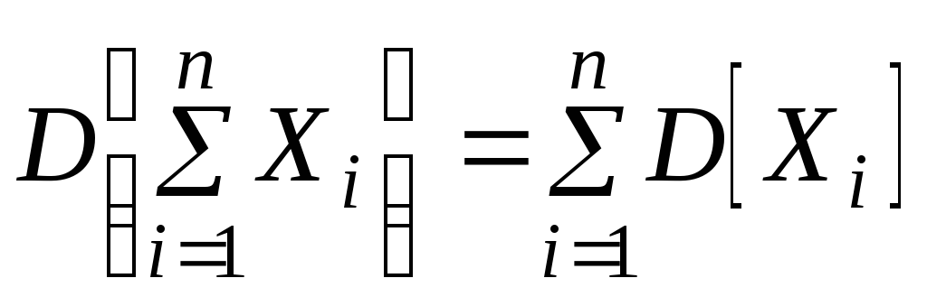
т.е.
дисперсия
суммы некоррелированных случайных
величин равна сумме дисперсий слагаемых.

Это
положение известно под названием теоремы
сложения дисперсий.

Теорема 9. Дисперсия
линейной конбинации случайных величин
определяется соотношением

(7.2.10)

где
К_ij—
корреляционный момент величин X_i,
X_j.

Доказательство.
Введем обозначение:

Тогда

(7.2.11)

Применяя
к правой части выражения (7.2.11) формулу
(7.2.7) для дисперсии суммы и учитывая, что
D[b]
= 0, получим:

(7.2.12)

где
— корреляционный момент величинY_i,
Y_j.

Вычислим этот
момент. Имеем:

аналогично

Отсюда

Подставляя это
выражение в (7.2.12), приходим к формуле
(7.2.10).

В
частном случае, когда все величины
(Х₁,Х₂,…,Х_n)
некоррелированные,
формула (7.2.10) принимает вид:

(7.2.13)

т.е.
дисперсия
линейной функции некоррелированных
случайных величин равна сумме произведений
квадратов коэффициентов на дисперсии
соответствующих аргументов).

Теорема 10.
Дисперсия произведения независимых
случайных величин определяется
соотношением

(7.2.14)

Доказательство.
Обозначим XY=Z.
По определению дисперсии

Так
как величины X,
Y
независимы,
m_z
= m_xm_y
и

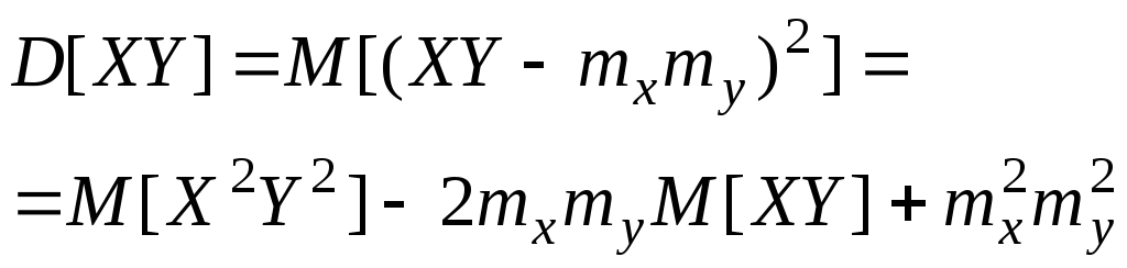
При
независимых X,
У величины
Х²,
Y²тоже
независимы следовательно,

(7.2.15)

Но
М[X²]
есть
не что иное, как второй начальный момент
величины X,
и,
следовательно, выражается через
дисперсию:

(7.2.16)

аналогично

(7.2.17)

Подставляя выражения
(7.2.16) и (7.2.17) в формулу (7.2.15) и приводя
подобные члены, приходим к формуле
(7.2.14).

В случае, когда
перемножаются центрированные случайные
величины (величины с математическими
ожиданиями, равными нулю), формула
(7.2.14) принимает вид:

(7.2.18)

т.е.
дисперсия
произведения независимых центрированных
случайных величин равна произведению
их дисперсий.

Соседние файлы в предмете [НЕСОРТИРОВАННОЕ]

Источник

Непрерывная случайная величина Х имеет Равномерный закон распределения на отрезке , если ее плотность вероятности Р(Х) постоянна на этом отрезке и равна нулю вне его, т. е.

Функция распределения случайной величины Х, распределенной по равномерному закону, есть

Математическое ожидание дисперсия а среднее квадратическое отклонение .

Пример 8.14. Поезда метрополитена идут регулярно с интервалом 3 мин. Пассажир выходит на платформу в случайный момент времени. Какова вероятность того, что ждать пассажиру придется не больше минуты. Найти математическое ожидание и среднее квадратическое отклонение случайной величины Х — времени ожидания поезда.

Решение. Случайная величина Х — время ожидания поезда на временном (в минутах) отрезке имеет равномерный закон распределения . Поэтому вероятность того, что пассажиру придется ждать не более минуты, равна От равной единице площади прямоугольника (рис. 8.11), т. е.

Мин,

мин.

Рис. 8.11

Пример 8.15. Найти математическое ожидание и дисперсию произведения двух независимых случайных величин ξ и η с равномерными законами распределения: ξ в интервале , η — в интервале .

Решение. Так как математическое ожидание произведения независимых случайных величин равно произведению их математических ожиданий, то . Для нахождения дисперсии воспользуемся формулой

найдем по формуле

Аналогично рассчитаем

Следовательно,

Пример 8.16. Вычислить математическое ожидание и дисперсию определителя

Элементы которого — независимые случайные величины с и

Решение. Вычислим математическое ожидание

Для нахождения дисперсии докажем, что если ξ и η — независимые случайные величины, то

Действительно,

Следовательно,

Замечание. Для определителя N-го порядка ;

Пример 8.17. Автоматический светофор работает в двух режимах: 1 мин. горит зеленый свет и 0,5 мин — красный и т. д. Водитель подъезжает к перекрестку в случайный момент времени. 1. Найти вероятность того, что он проедет перекресток без остановки. 2. Составить закон распределения и вычислить числовые характеристики времени ожидания у перекрестка.

Решение. 1. Момент проезда автомобиля T через перекресток распределен равномерно в интервале, равном периоду смены цветов светофора. Этот период равен 1 + 0,5 = 1,5 мин. Для того чтобы машина проехала через перекресток не останавливаясь, достаточно того, чтобы момент проезда пришелся на интервал времени . Тогда

2. Время ожидания является смешанной случайной величиной: с вероятностью она равна нулю, а с вероятностью принимает с равномерной плотностью вероятностей любые значения между 0 и 0,5 мин; тогда график функции распределения случайной величины имеет вид, изображенный на рис. 8.12: