Как найти дугу эллипса - Исправление недочетов и поиск решений вместе с Examum.ru

Как ни странно, но для нахождения длины дуги эллипса нет какой-то определенной функции, как в случае длины дуги окружности, или нахождения координат точки на эллипсе. Это интегральное уравнение.

Калькулятор

Давайте вначале посчитаем, оценим.

Если есть вопросы, предложения по калькулятору или заметили ошибку, буду очень рад обратной связиx

Потом разберем разные подходы к решению. Оранжевый маркер задает стартовый угол дуги, красный — отклонение. Справа сверху в качестве оценочного параметра представлен периметр, посчитанный по второй формуле Рамануджана.

Эллипс:

a:
b:

Параметры дуги:

Get a better browser, bro…

Интегральное уравнение будем решать как обычно делается в подобных случаях: суммировать очень маленькие значения, которые получаются в результате работы некоей функции, на заданном диапазоне данных, которые наращиваются на чрезвычайно малую постоянную величину. Эта малая величина задается вызывающей стороной. В конце статьи есть рабочий пример с исходниками, в котором можно поиграться с этой «малостью».

Длина дуги, как сумма хорд

Самое простое, что может прийти в голову, это двигаться от начала дуги к ее концу с небольшим наращиванием угла отклонения, считать хорду и прибавлять ее к накапливаемой сумме.

Рис.1. Сумма хорд

Формула такова:

(1) Сумма хорд

Проще говоря, находим координаты двух точек на эллипсе, отстоящих друг от друга на некий малый угол, по ним находим хорду, как гипотенузу получившегося прямоугольного треугольника.

В коде выглядит так:

//*****************************************************************

// Нахождение длины дуги эллипса, заданного прямоугольником ARect

// По аналогии с GDI+, углы в градусах, по часовой. Хордами

// ∑ √ (Δx² + Δy²)

//*****************************************************************

function CalcArcEllipseLen1(ARect : TxRect; // эллипс

startAngle : Extended; // старт.угол

sweepAngle : Extended; // угол дуги

deltaAngle : Extended=0.01 // дискрета

): Extended;

var tmp : Extended; // наращиваемый угол

pnt : TxPoint; // новые координаты по tmp

val : TxPoint; // координаты в предыдущей итерации

dw : Extended; // убывающий параметр цикла

l : extended; // длина текущей хорды

begin

// переводим градусы в радианы

startAngle := startAngle * pi/180;

sweepAngle := sweepAngle * pi/180;

deltaAngle := deltaAngle * pi/180;

// инициализируем

tmp := startAngle;

dw := sweepAngle;

result := 0;

// стартовая координата

val := CalcEllipsePointCoord(ARect,tmp);

repeat

// уменьшаем параметр цикла

dw := dw — deltaAngle;

// определяем значение угла

if dw < 0 then tmp := tmp + (deltaAngle+dw)

else tmp := tmp + deltaAngle;

// считаем новую точку на эллипсе

pnt := CalcEllipsePointCoord(ARect,tmp);

// длина хорды

l := sqrt(sqr(val.X—pnt.x)+sqr(val.Y—pnt.y));

// сумма, интеграл

result := result+l;

val := pnt;

until dw < 0;

end;

Проверим с планетарным размахом. По последним данным Международной Службы Вращения Земли (IERS — 1996) большая экваториальная полуось Земли равна 6 378 136,49 м, а полярная малая — 6 356 751,75 м.

Посчитаем периметр меридиана каким-нибудь онлайн-калькулятором, получаем 40 007 859.543 (некоторые могут дать другое число, т.к. используют приближенные формулы для вычисления периметра).

Представленная выше функция за 109 милисекунд выдала результат 40 007 996.265 при дельте 0.001. Это нельзя назвать точным результатом.

Длина дуги, как интеграл

Длиной некоторой дуги называется тот предел, к которому стремится длина вписанной ломаной, когда длина наибольшего ее звена стремится к нулю:

(2) Предел суммы хорд при максимальной длине хорды, стремящейся к нулю

(3) Длина t-го звена (хорды) вписанной ломаной

Таким образом, длина дуги эллипса может быть описана интегральным уравнением:

(4) Интегрально-дифференциальное уравнение дуги эллипса

Используя параметрическое уравнение эллипса, приходим к уравнению:

Где t1 и t2 – параметры для начала и конца дуги параметрического уравнения эллипса. Параметром является некий угол к оси абсцисс. Что такое и как найти параметр для угла эллипса подробно изложено тут.

Зная, что (cos t)’ = — sin t, (sin t)’ = cos t (подробный вывод приведен тут и тут), получаем следующую формулу:

(5) Длина дуги эллипса

Выводов достаточно, чтобы написать вторую функцию нахождения длины дуги эллипса.

// Получить разницу между углами A2-A1

function CalcSweepAngle (A1,A2 : Extended;

ANormalize : boolean = true) : Extended;

begin

result := A2—A1;

if (result < 0) and (ANormalize) then

result := 2*pi + result;

end;

//*****************************************************************

// Нахождение длины дуги эллипса, заданного через a и b

// Сумма от корня суммы квадратов производных, через sin/cos по ∂t

// ∑ [√(∂x²/∂t² + ∂y²/∂t²)] ∂t

//*****************************************************************

function CalcArcEllipseLen2(

a,b : extended; // полуоси

startAngle : Extended; // старт.угол

sweepAngle : Extended; // угол откл.

deltaAngle : Extended=0.01 // дискрета

): Extended;

var sn,cs: Extended;// синус, косинус

tmp : Extended; // наращиваемый угол

bet : Extended; // старый параметр

dw : Extended; // убывающий параметр цикла

t : Extended; // новый параметр

l : extended; // значение функции в t

begin

// переводим градусы в радианы

startAngle := startAngle * pi/180;

sweepAngle := sweepAngle * pi/180;

deltaAngle := deltaAngle * pi/180;

// инициализируем

tmp := startAngle;

dw := sweepAngle;

result := 0;

// параметр для начального угла

SinCos(tmp,sn,cs);

bet := ArcTan2(a*sn, b*cs);

repeat

// уменьшаем параметр цикла

dw := dw — deltaAngle;

// определяем значение угла

if dw < 0 then

tmp := tmp + (deltaAngle+dw)

else tmp := tmp + deltaAngle;

// находим параметр для угла

SinCos(tmp,sn,cs);

t := ArcTan2(a*sn, b*cs);

// разница между параметрами dt=t-bet

bet := CalcSweepAngle(bet,t);

// эллиптический интеграл II рода

SinCos(t,sn,cs);

l := sqrt ( sqr(a)*sqr(sn) + sqr(b)*sqr(cs))*bet;

// запоминаем параметр

bet := t;

// сумма, интеграл

result := result+l;

until dw <= 0;

end;

Результат при dt = 0.001 равен 40 007 859,543 за 109 милисекунд. Отлично!

Длина дуги через эксцентриситет

Это еще не окончательный вид уравнения. В ряде интересных параметров для эллипса есть такая числовая характеристика, показывающая степень отклонения эллипса от окружности, как эксцентриситет. Формула для эллипса:

(6) Эксцентриситет эллипса через полуоси

Чем эксцентриситет ближе к нулю, т.е. разница между a и b меньше, тем больше эллипс похож на окружность и наоборот, чем эксцентриситет ближе к единице, тем он более вытянут.

Выразим b² = a²(1 — e²), подставим в формулу (5), помним, что sin²t + cos²t = 1 (справочник [1]), убираем a² за знак корня, и, как постоянную величину, за знак интеграла тоже, получаем:

(7) Окончательный вид уравнения для длины дуги эллипса

Пишем функцию, ожидаем более шустрого выполнения:

//*****************************************************************

// Нахождение длины дуги эллипса, заданного через a и b

// По аналогии с GDI+, углы в градусах, по часовой. Считаем E(t,e)

// a ∑ [√(1-e²cos²t)] ∂t

//*****************************************************************

function CalcArcEllipseLen3(

a,b : extended; // полуоси

startAngle : Extended; // старт.угол

sweepAngle : Extended; // угол откл.

deltaAngle : Extended=0.01 // дискрета

): Extended;

var sn,cs: Extended;// синус, косинус

tmp : Extended; // наращиваемый угол

bet : Extended; // старый параметр

dw : Extended; // убывающий параметр цикла

ex : Extended; // эксцентриситет

t : Extended; // новый параметр

l : extended; // значение функции в t

begin

// переводим градусы в радианы

startAngle := startAngle * pi/180;

sweepAngle := sweepAngle * pi/180;

deltaAngle := deltaAngle * pi/180;

// считаем эксцентриситет

ex := 1 —sqr(b)/sqr(a);

// инициализируем

tmp := startAngle;

dw := sweepAngle;

result := 0;

// параметр для начального угла

SinCos(tmp,sn,cs);

bet := ArcTan2(a*sn, b*cs);

repeat

// уменьшаем параметр цикла

dw := dw — deltaAngle;

// определяем значение угла

if dw < 0 then

tmp := tmp + (deltaAngle+dw)

else tmp := tmp + deltaAngle;

// находим параметр для угла

SinCos(tmp,sn,cs);

t := ArcTan2(a*sn, b*cs);

// разница между параметрами dt=t-bet

bet := CalcSweepAngle(bet,t);

// эллиптический интеграл II рода

l := sqrt (1—ex*sqr(cos(t)))*bet;

// запоминаем параметр

bet := t;

// сумма, интеграл

result := result+l;

until dw <= 0;

result := a*result;

end;

Результат 40 007 859.543, за чуть меньшее время, 94 милисекунды.

Длина дуги через эксцентриситет с подготовкой

Возьмем за основу последнюю функцию. Алгоритм построен так, что в цикле идем от стартового угла, к конечному, на каждой итерации подсчитывая параметр. А если сразу посчитать начальный и конечный параметры и определить условие выхода из цикла? Этим мы однозначно снизим вычислительную нагрузку внутри цикла.

Рис.2. Параметры дуги эллипса.

То есть, вместо того, чтобы идти из точки A в точку B, мы заранее считаем параметры t1 и t2. И в цикле больше нахождением параметров не занимаемся, а только считаем очередное приращение.

Берем код последней реализации и улучшаем:

//*****************************************************************

// Нахождение длины дуги эллипса, заданного через a и b

// По аналогии с GDI+, углы в градусах, по часовой. Считаем E(t,e)

// a ∑ [√(1-e²cos²t)] ∂t

// Но параметры и угол отклонения параметра считаем заранее

//*****************************************************************

function CalcArcEllipseLen4(

a,b : extended; // полуоси

startAngle : Extended; // старт.угол

sweepAngle : Extended; // угол откл.

deltaAngle : Extended=0.01 // дискрета

): Extended;

var sn,cs: Extended;// синус, косинус

tmp : Extended; // наращиваемый угол

bet : Extended; // старый параметр

dw : Extended; // убывающий параметр цикла

ex : Extended; // эксцентриситет

l : extended; // значение функции в t

begin

// переводим градусы в радианы

startAngle := startAngle * pi/180;

sweepAngle := sweepAngle * pi/180;

deltaAngle := deltaAngle * pi/180;

// считаем эксцентриситет

ex := 1 —sqr(b)/sqr(a);

// инициализируем

tmp := startAngle;

result := 0;

// параметр для начального угла

SinCos(tmp,sn,cs);

bet := ArcTan2(a*sn, b*cs);

// считаем параметр для цикла

SinCos(tmp+sweepAngle,sn,cs);

dw := ArcTan2(a*sn, b*cs);

dw := CalcSweepAngle(bet, dw);

// для корректной работы цикла, запоминаем в бет старт.параметр

tmp := bet;

// если sweepAngle = 360, результат будет равен 0

// если sweepAngle > 360, результат будет от оставшейся разницы

if sweepAngle >= 2*pi then

dw := 2*pi + dw;

repeat

// уменьшаем параметр цикла

dw := dw — deltaAngle;

bet := tmp;

// определяем значение угла

if dw < 0 then tmp := tmp + (deltaAngle+dw)

else tmp := tmp + deltaAngle;

// разница между параметрами dt=tmp-bet

bet := CalcSweepAngle(bet,tmp);

// эллиптический интеграл II рода

l := sqrt (1—ex*sqr(cos(tmp)))*bet;

// сумма, интеграл

result := result+l;

until dw <= 0;

result := a*result;

end;

Результат — 40 007 859,543 за 30 милисекунд! Мысль явно здравая.

Длина дуги и хорошо забытые хорды

Но вернемся к сумме хорд. Что там-то не так? Казалось бы, все просто, понятно и должно работать, но результат, мягко говоря, не точен.

Работая с вещественными типами, результат зависит от «мелкости» приращения, от разрядности используемых типов. Накапливаемые погрешности, неточное представление дробного числа и прочие прелести чисел с плавающей запятой.

Тип Extended – самый точный из существующих в Delphi (и, как следствие, самый медленный). Перепишем нахождение длины дуги хордами, используя этот тип, и без вызовов внешних функций нахождения координат на эллипсе.

//*****************************************************************

// Нахождение длины дуги эллипса, заданного через a и b

// По аналогии с GDI+, углы в градусах, по часовой. Считаем хордами

// Абсолютно то же самое, что (1), но типы и точность изменены

// ∑ √ (Δx² + Δy²)

//*****************************************************************

function CalcArcEllipseLen5(

a,b : extended; // полуоси

startAngle : Extended; // старт.угол

sweepAngle : Extended; // угол откл.

deltaAngle : Extended=0.01 // дискрета

): Extended;

var sn,cs: Extended;// синус, косинус

tmp : Extended; // наращиваемый угол

dw : Extended; // убывающий параметр цикла

l : extended; // длина текущей дуги

vx,vy : extended;

px,py : Extended;

begin

// переводим градусы в радианы

startAngle := startAngle * pi/180;

sweepAngle := sweepAngle * pi/180;

deltaAngle := deltaAngle * pi/180;

// инициализируем

tmp := startAngle;

dw := sweepAngle;

result := 0;

// находим параметр (некий угол) для уравнения

SinCos(tmp,sn,cs);

SinCos (ArcTan2(a*sn, b*cs), sn, cs);

vX := a * cs;

vY := b * sn;

repeat

// уменьшаем параметр цикла

dw := dw — deltaAngle;

// определяем значение угла

if dw < 0 then tmp := tmp + (deltaAngle+dw)

else tmp := tmp + deltaAngle;

// считаем новую точку на эллипсе

SinCos(tmp,sn,cs);

SinCos (ArcTan2(a*sn,b*cs),sn,cs);

pX := a * cs;

pY := b * sn;

// длина хорды

l := sqrt(sqr(pX—vx)+sqr(pY—vy));

// сумма, интеграл

result := result+l;

vx := px;

vy := py;

until dw < 0;

end;

Результат 40 007 859.542 за 94 милисекунды. Разница в одну тысячную, и такое же время. Весьма неплохо!

Практика

Скачать исходник + исполняемый файл

Качаем, запускаем. Видим такое окно:

Рис.3. Пример: Вид при запуске

При запуске в полях полуосей находятся «земные» значения. Эллипс сильно смахивает на окружность. Можно сразу нажать «Расчет», увидеть значения полярного меридиана, и начинать уже эксперименты.

Для начала проверим корректность получаемых результатов. Я попытался найти какие-нибудь онлайн калькуляторы для подсчета длины дуги эллипса, в которых можно было бы указать стартовый угол и произвольное отклонение, либо просто пару углов, определяющих дугу. Но все калькуляторы считают периметр эллипса. А с произвольной дугой как-то… не встретились.

Картинка из вики:

Длина дуги эллипса (s) в зависимости от его параметра (θ) Автор: Illustr — собственная работа, CC BY-SA 4.0, Ссылка

Заскриним несколько моментов и посчитаем корректность:

Рис.4. Скрины расчетов

Введем a=2, b=0.5, стартовый угол равен 0, отклонение θ=5.642.

Рис.5. Подсчет длины дуги для a=2, b=0.5, стартовый угол=0, отклонение θ=5.642

Видим результат у всех один 8.055. Т.е правы все.

Аналогично поступаем с остальными тремя скринами:

отклонение θ=1.154. У нас получился результат 1.333. На скрине видим результат s=1.334. Как так? Давайте увеличим «Дельту» в 10 раз, т.е. вместо 0.001, сделаем 0,01. У всех интегральных 2) 3) 4) результат станет 1.334. В то время, как у 1) и 5), т.е. примитивно-неинтегрально-хордовых останется 1.333.

Какой результат более истинный? Смотрите сами. Уменьшение дельты, т.е. угла для подсчетов, ведет к более точному результату. На 0.001 интегральные функции выдали результат как хордовые. При более грубой дельте, интегральные чуть изменились, а хордовые верны своему результату.

Сделаем дельту очень мелкой, равной 0.00001. Результат у всех, кроме первой, тот же, 1.333.

Лично я начинаю верить 5-ой формуле.

отклонение θ= 206. У нас получился результат 4.322. На скрине результат s= 4.322. Дельта 0.001. Все отлично.
отклонение θ= 4,488. У нас получился результат 5,989. На скрине результат s= 5,989. Дельта 0.001. Все отлично.

Вывод : Формулы 2-5 работают как надо. Фаворит 5. За меньшее время, т.е. при более «грубой» дельте, находит правильный результат.

Проверим на ужасных эллипсах. Т.е. где эксцентриситет очень близок к единице.

Рис.6. Проверка на очень «сплющенном» эллипсе

Можем заметить следующее: при 0.00001 функции 2 и 3 дали результат, близкий к результату функции 4, полученный при дельте 0.001. При дельте 0.00001 функция 4 дала результат, близкий к результату функции 5. Сама же функция 5 слабо колеблется в показаниях, что при дельте в 0.001, что при 0.00001.

Аналогичную ситуацию можно пронаблюдать при сильно вытянутом эллипсе:

Рис.7. Проверка на очень «вытянутом» эллипсе

Таким образом, имеет смысл использовать функции 4 и 5. Одну, как представительницу интегрального сословия, самую быструю и более точную из них. Другую, как представительницу очевидного и простого метода, работающую, между тем, лучше своих интегральных коллег при минимальных ресурсных затратах.

Небольшая инструкция

Правая кнопка мыши задает стартовый угол. Удерживая правую кнопку мыши можно «прогуляться» по эллипсу. Конечная точка дуги будет следовать за стартовой точкой, отстоя на заданный ранее угол. Если поставить галку на «сохранять параметрическое отклонение», параметрический угол между t1 и t2 станет неизменен. Очень полезно пронаблюдать, как будет меняться сектор.

Левая кнопка мыши задает конечную точку дуги, т.е. угол отклонения.

Скачать

Скачать исходник + исполняемый файл

Друзья, спасибо за внимание!

Подписывайтесь на телегу.

Надеюсь, материал был полезен.

Источник

Определение эллипсa

Определение.

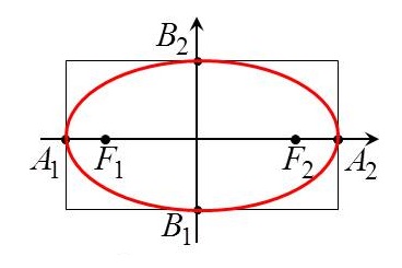
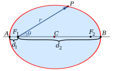
Эллипс — это замкнутая плоская кривая, сумма расстояний от каждой точки которой до двух точек F₁ и F₂ равна постоянной величине. Точки F₁ и F₂ называют фокусами эллипса.

F₁M₁ + F₂M₁ = F₁M₂ + F₂M₂ = A₁A₂ = const

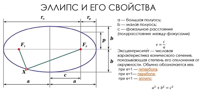
Элементы эллипсa

F₁ и F₂ — фокусы эллипсa

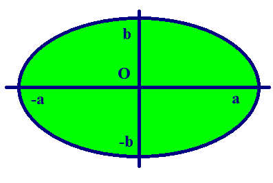
Оси эллипсa.

А₁А₂ = 2a — большая ось эллипса (проходит через фокусы эллипса)

B₁B₂ = 2b — малая ось эллипса (перпендикулярна большей оси эллипса и проходит через ее центр)

a — большая полуось эллипса

b — малая полуось эллипса

O — центр эллипса (точка пересечения большей и малой осей эллипса)

Вершины эллипсa A₁, A₂, B₁, B₂ — точки пересечения эллипсa с малой и большой осями эллипсa

Диаметр эллипсa — отрезок, соединяющий две точки эллипса и проходящий через его центр.

Фокальное расстояние c — половина длины отрезка, соединяющего фокусы эллипсa.

Эксцентриситет эллипсa e характеризует его растяженность и определяется отношением фокального расстояния c к большой полуоси a. Для эллипсa эксцентриситет всегда будет 0 < e < 1, для круга e = 0, для параболы e = 1, для гиперболы e > 1.

Фокальные радиусы эллипсa r₁, r₂ — расстояния от точки на эллипсе до фокусов.

Радиус эллипсa R — отрезок, соединяющий центр эллипсa О с точкой на эллипсе.

R =	ab	=	b
√a²sin²φ + b²cos²φ	√1 — e²cos²φ

где e — эксцентриситет эллипсa, φ — угол между радиусом и большой осью A₁A₂.

Фокальный параметр эллипсa p — отрезок который выходит из фокуса эллипсa и перпендикулярный большой полуоси:

Коэффициент сжатия эллипсa (эллиптичность) k — отношение длины малой полуоси к большой полуоси. Так как малая полуось эллипсa всегда меньше большей, то k < 1, для круга k = 1:

k = √1 — e²

где e — эксцентриситет.

Сжатие эллипсa (1 — k ) — величина, которая равная разности между единицей и эллиптичностью:

Директрисы эллипсa — две прямые перпендикулярные фокальной оси эллипса, и пересекающие ее на расстоянии

от центра эллипса. Расстояние от фокуса до директрисы равно

Основные свойства эллипсa

1. Угол между касательной к эллипсу и фокальным радиусом r₁ равен углу между касательной и фокальным радиусом r₂ (Рис. 2, точка М₃).

2. Уравнение касательной к эллипсу в точке М с координатами (x_M, y_M):

3. Если эллипс пересекается двумя параллельными прямыми, то отрезок, соединяющий середины отрезков образовавшихся при пересечении прямых и эллипса, всегда будет проходить через центр эллипсa. (Это свойство дает возможность построением с помощью циркуля и линейки получить центр эллипса.)

4. Эволютой эллипсa есть астероида, что растянута вдоль короткой оси.

5. Если вписать эллипс с фокусами F₁ и F₂ у треугольник ∆ ABC, то будет выполнятся следующее соотношение:

1 =	F₁A ∙ F₂A	+	F₁B ∙ F₂B	+	F₁C ∙ F₂C
CA ∙ AB	AB ∙ BC	BC ∙ CA

Уравнение эллипсa

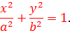
Каноническое уравнение эллипсa:

Уравнение описывает эллипс в декартовой системе координат. Если центр эллипсa О в начале системы координат, а большая ось лежит на абсциссе, то эллипсa описывается уравнением:

Если центр эллипсa О смещен в точку с координатами (x_o, y_o), то уравнение:

1 =	(x — x_o)²	+	(y — y_o)²
a²	b²

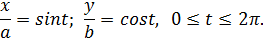
Параметрическое уравнение эллипсa:

{	x = a cos α	де 0 ≤ α < 2π
y = b sin α

Радиус круга вписанного в эллипс

Круг, вписан в эллипс касается только двух вершин эллипсa B₁ и B₂. Соответственно, радиус вписанного круга r будет равен длине малой полуоси эллипсa OB₁:

r = b

Радиус круга описанного вокруг эллипсa

Круг, описан вокруг эллипсa касается только двух вершин эллипсa A₁ и A₂. Соответственно, радиус описанного круга R будет равен длине большой полуоси эллипсa OA₁:

R = a

Площадь эллипсa

Формула определение площади эллипсa:

S = πab

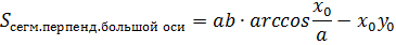
Площадь сегмента эллипсa

Формула площади сегмента, что находится по левую сторону от хорды с координатами (x, y) и (x, -y):

S =	πab	—	b	(	x	√	a² — x² + a² ∙ arcsin	x	)
2	a	a

Периметр эллипсa

Найти точную формулу периметра эллипсa L очень тяжело. Ниже приведена формула приблизительной длины периметра. Максимальная погрешность этой формулы ~0,63 %:

L ≈ 4	πab + (a — b)²
a + b

Длина дуги эллипсa

Формулы определения длины дуги эллипсa:

1. Параметрическая формула определения длины дуги эллипсa через большую a и малую b полуоси:

	t₂
l =	∫	√a²sin²t + b²cos²t dt
	t₁

2. Параметрическая формула определения длины дуги эллипсa через большую полуось a и эксцентриситет e:

	t₂
l =	∫	√1 — e²cos²t dt, e < 1
	t₁

Источник

Эллипс — свойства, уравнение и построение фигуры

Среди центральных кривых второго порядка особое место занимает эллипс, близкий к окружности, обладающий похожими свойствами, но всё же уникальный и неповторимый.

Определение и элементы эллипса

Множество точек координатной плоскости, для каждой из которых выполняется условие: сумма расстояний до двух заданных точек (фокусов) есть величина постоянная, называется эллипсом.

По форме график эллипса представляет замкнутую овальную кривую:

Наиболее простым случаем является расположение линии так, чтобы каждая точка имела симметричную пару относительно начала координат, а координатные оси являлись осями симметрии.

Отрезки осей симметрии, соединяющие две точки эллипса, называются осями. Различаются по размерам (большая и малая), а их половинки, соответственно, считаются полуосями.

Точки эллипса, являющиеся концами осей, называются вершинами.

Расстояния от точки на линии до фокусов получили название фокальных радиусов.

Расстояние между фокусами есть фокальное расстояние.

Отношение фокального расстояния к большей оси называется эксцентриситетом. Это особая характеристика, показывающая вытянутость или сплющенность фигуры.

Основные свойства эллипса

имеются две оси и один центр симметрии;

при равенстве полуосей линия превращается в окружность;

все точки фигуры лежат внутри прямоугольника со сторонами, равными большой и малой осям эллипса, проходящими через вершины параллельно осям.

Уравнение эллипса

Пусть линия расположена так, чтобы центр симметрии совпадал с началом координат, а оси – с осями координат.

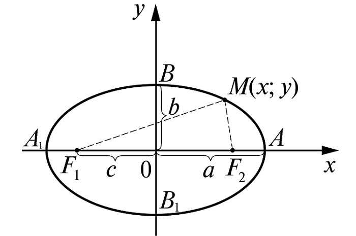
Для составления уравнения достаточно воспользоваться определением, введя обозначение:

а – большая полуось (в наиболее простом виде её располагают вдоль оси Оx) (большая ось, соответственно, равна 2a);

c – половина фокального расстояния;

M(x;y) – произвольная точка линии.

В этом случае фокусы находятся в точках F₁(-c;0); F₂(c;0)

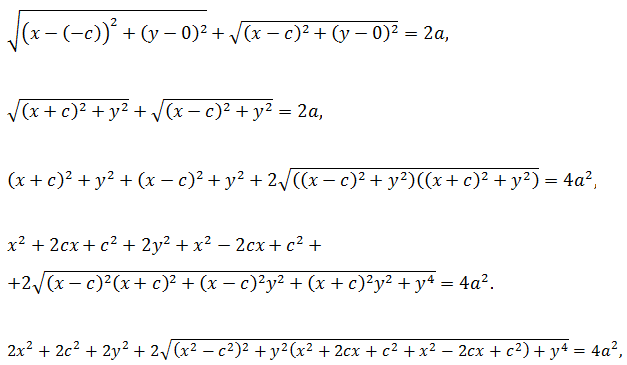
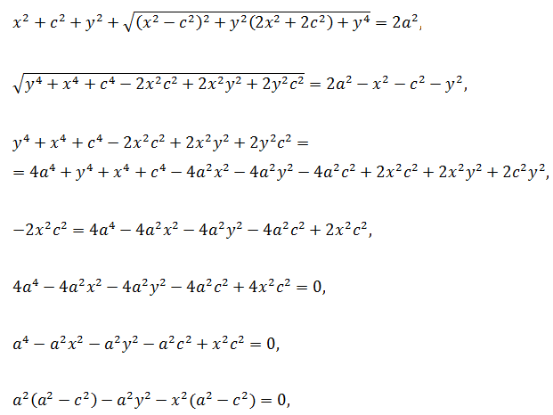
После ввода ещё одного обозначения

получается наиболее простой вид уравнения:

a 2 b 2 — a 2 y 2 — x 2 b 2 = 0,

a 2 b 2 = a 2 y 2 + x 2 b 2 ,

Параметр b численно равен полуоси, расположенной вдоль Oy (a > b).

В случае (b b) формула эксцентриситета (ε) принимает вид:

Чем меньше эксцентриситет, тем более сжатым будет эллипс.

Площадь эллипса

Площадь фигуры (овала), ограниченной эллипсом, можно вычислить по формуле:

a – большая полуось, b – малая.

Площадь сегмента эллипса

Часть эллипса, отсекаемая прямой, называется его сегментом.

Длина дуги эллипса

Длина дуги находится с помощью определённого интеграла по соответствующей формуле при введении параметра:

Радиус круга, вписанного в эллипс

В отличие от многоугольников, круг, вписанный в эллипс, касается его только в двух точках. Поэтому наименьшее расстояние между точками эллипса (содержащее центр) совпадает с диаметром круга:

Радиус круга, описанного вокруг эллипса

Окружность, описанная около эллипса, касается его также только в двух точках. Поэтому наибольшее расстояние между точками эллипса совпадает с диаметром круга:

Онлайн калькулятор позволяет по известным параметрам вычислить остальные, найти площадь эллипса или его части, длину дуги всей фигуры или заключённой между двумя заданными точками.

Как построить эллипс

Построение линии удобно выполнять в декартовых координатах в каноническом виде.

Строится прямоугольник. Для этого проводятся прямые:

Сглаживая углы, проводится линия по сторонам прямоугольника.

Полученная фигура есть эллипс. По координатам отмечается каждый фокус.

При вращении вокруг любой из осей координат образуется поверхность, которая называется эллипсоид.

Чертежик

Построение овала

Рассмотрим построение овала двумя методами: окружности и параллелограмма.

Воспользуемся методом окружности.

1.) Начинаем чертить с построения осей.

2.) Чертим окружность

3.) Чертим дуги ЕА и BD радиусом ЕС

4.) Чертим дуги ED и AB радиусом FB

Применим метод параллелограмма.

1.) Начинаем с построения осевых линий

2.) Чертим линии параллельные осевым линиям. Где d — диаметр окружности.

3.) Строим дуги HB и DF радиусом HE4.) Продолжаем с черчения дуги BD радиуса MB и дуги FH радиусом PH

Применение построения овала на чертежах вы можете посмотреть здесь

Урок 3. Окружность в перспективе. Как нарисовать кружку и вазу

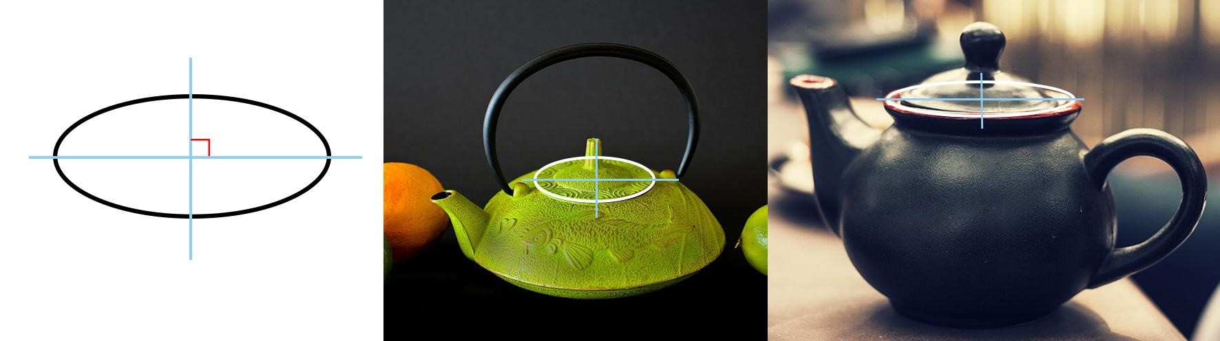
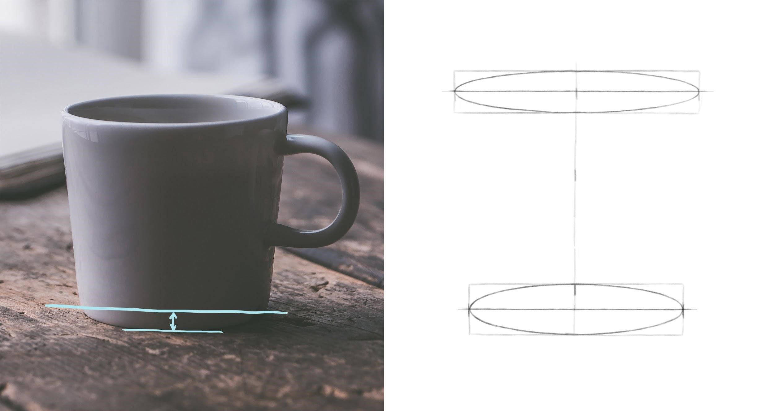
В этом уроке мы разберемся, как изображать объекты, в основе которых лежат окружности: чайник, вазу, бокал, кувшин, колонну, маяк. Сложность их изображения в пространстве заключается в том, что принцип равноудаленности точек окружности от центра срабатывает, только когда мы смотрим на плоскость прямо (то есть направление взгляда перпендикулярно ей). Например, мы видим круглый циферблат часов перед собой или чашку и блюдце, когда наклонились над ними. В других случаях (взгляд падает на плоскость под углом) мы видим искажение формы окружности, ее превращение в овал (эллипс).

Содержание:

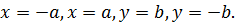
Ненадолго вернемся к коробкам из прошлого урока. Только теперь рассмотрим кубическую форму. Обратите внимание, как квадраты плоскостей, уходящих вдаль, сплющиваются. Верхние и нижние грани превращаются в трапеции. И тем сильнее они сужаются по вертикальной оси, чем ближе находятся к уровню глаз (к линии горизонта).

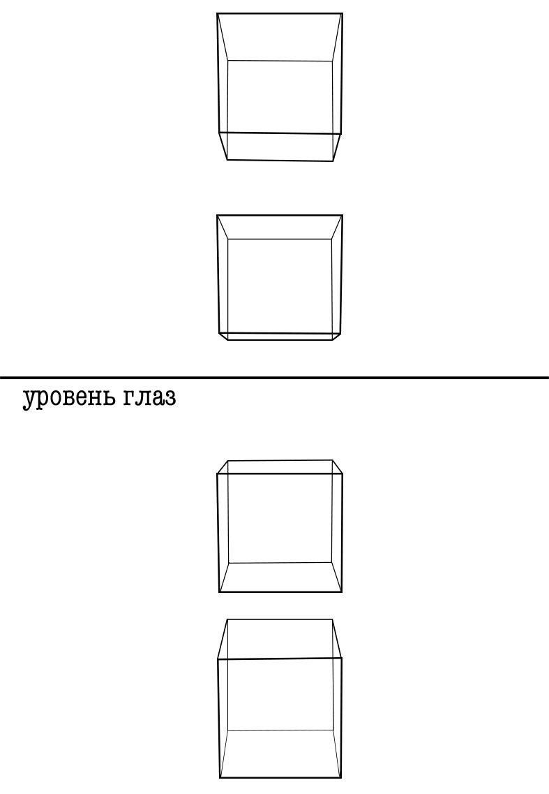
То же самое происходит и с окружностями. Чем дальше от линии горизонта они находятся, тем больше они открываются (обратите внимание на верхние и нижние плоскости этих спилов). А на уровне глаз окружность сужается до линии. Мы видим лишь переднюю грань предмета.

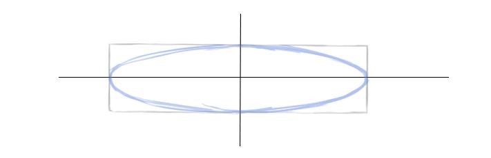
Принципы рисования эллипсов:

Принцип 1. У эллипса есть две оси симметрии: большая и малая. Они перпендикулярны. Здесь будем работать с наиболее частым случаем – когда предмет расположен прямо, то есть вертикальная ось (малая) находится под углом в 90°, а горизонтальная (большая) – под углом в 180°.

Принцип 2. У эллипса 4 вершины (они лежат на пересечении с осями). Эти точки в наибольшей степени удалены от центра. Форма эллипса выглядит искаженной, если соседние с вершинами точки смещены на тот же уровень (на эллипсе справа показано красным цветом).

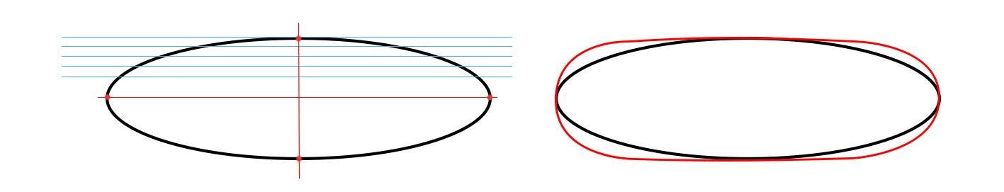
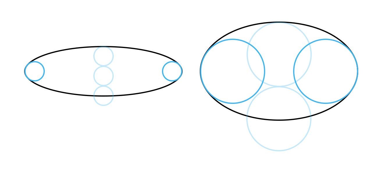
Принцип 3. Другая крайность – это заострение боков эллипсов. Они должны быть скругленными. В бока можно вписать окружности. И чем больше раскрыт эллипс, тем больше диаметр этой окружности относительно высоты эллипса (на примере ниже это сравнение показано бледно-голубым цветом).

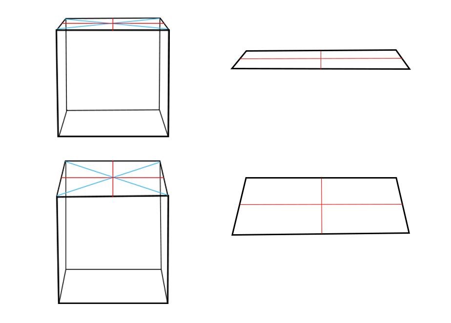
Принцип 4. Центр эллипса смещен вдаль (вверх) относительно геометрического центра из-за перспективного искажения. То есть ближняя половина эллипса больше дальней. Однако обратите внимание, что это смещение очень незначительно. Разберем, почему. Начнем с квадратов, поскольку круг вписывается в эту форму. Ниже показаны кубы, справа их верхние квадратные грани в перспективе. Проведены оси красным. Сравните, насколько их ближние половины больше дальних. Разница очень небольшая. То же самое будет и для эллипсов, вписанных в них. Ошибочно преувеличивать в рисунках эту разницу между ближней и дальней половинками эллипсов.

Рисуем эллипсы

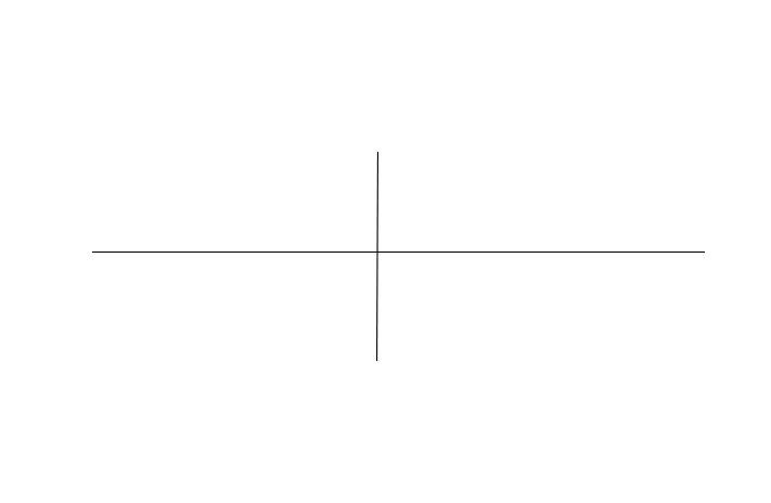
Шаг 1. Для начала проведем две перпендикулярных оси.

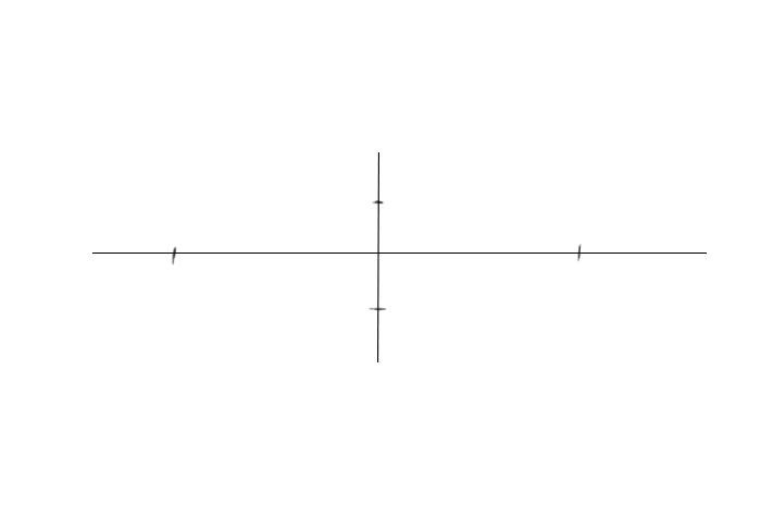
Шаг 2. Отметим границы произвольного эллипса симметрично по горизонтальной оси. А для вертикальной верхнюю половину (дальнюю) сделаем чуть-чуть меньше нижней.

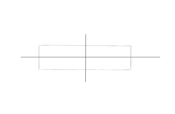
Шаг 3. Нарисуем по этим отметкам прямоугольник, в который будем вписывать эллипс.

Шаг 4. Наметим легкие дуги в местах пересечения осей и прямоугольника.

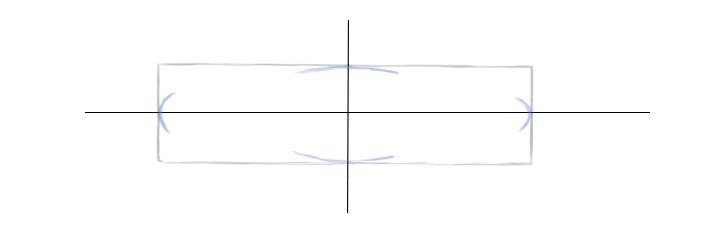
Шаг 5. Соединим легкими линиями эти дуги, стараясь изобразить эллипс более симметрично.

Шаг 6. По обозначенному пути проведем более четкую линию. Смягчим ластиком лишнее.

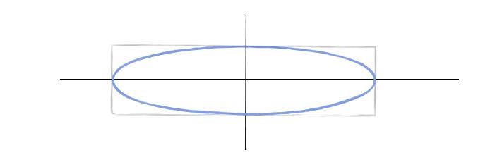
Более правильно было бы при рисовании эллипса вписывать его в квадратную плоскость в перспективе, то есть в трапецию. Однако, во-первых, сложно точно построить такую трапецию, зная лишь вершины эллипса. А во-вторых, овал, вписанный в квадрат в перспективе, мало отличается от вписанного в прямоугольник по тем же самым вершинам.

Рисуем кружку

Шаг 1. Начинаем с общих пропорций предмета. Измеряем, сколько раз ширина кружки (ее верха) умещается в высоте. Можно пока не учитывать ручку, однако надо оставить для нее достаточно места на листе. Намечаем общие габариты. Находим середину предмета по ширине и проводим через нее вертикальную ось. Чтобы нарисовать ее ровно, удобно сделать 2-3 вспомогательные отметки по высоте предмета на том же расстоянии от ближнего края листа, что и первая отметка середины предмета.

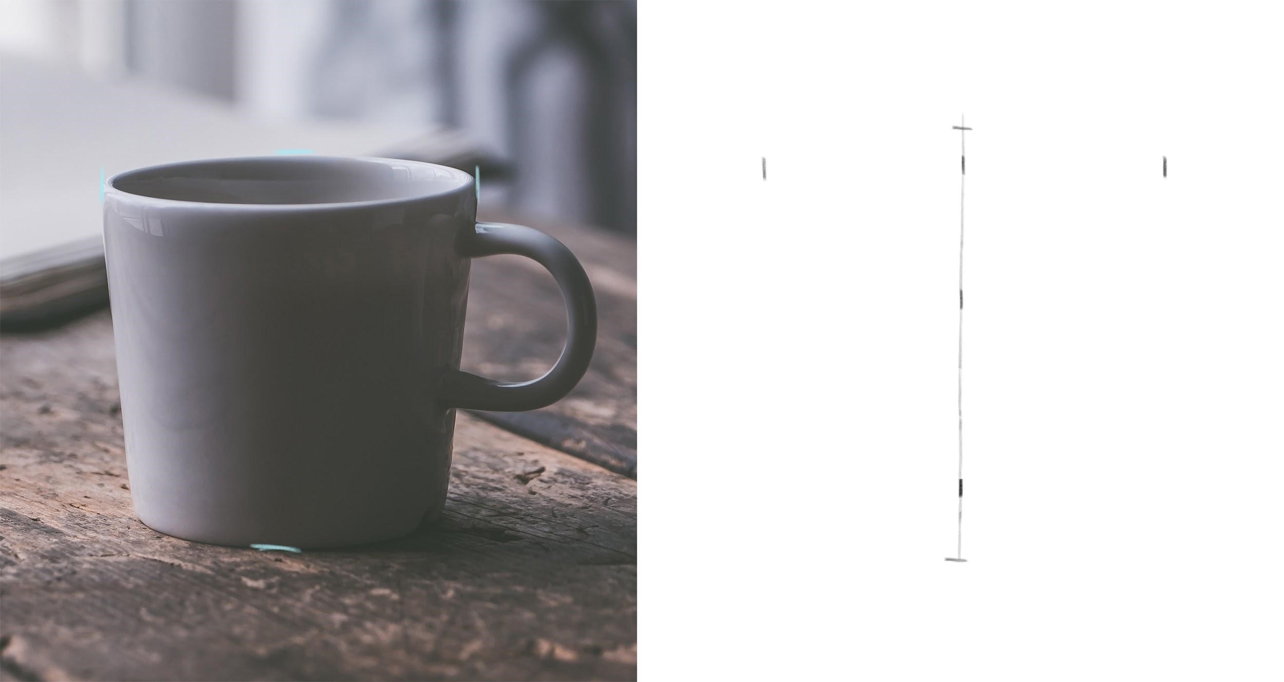
Шаг 2. Найдем высоту верхнего эллипса. Для этого измерим, сколько раз она умещается в его ширине (которую мы нашли ранее). Отметим нижнюю границу эллипса от верхнего края кружки. Легкими линиями нарисуем прямоугольник по намеченным крайним точкам.

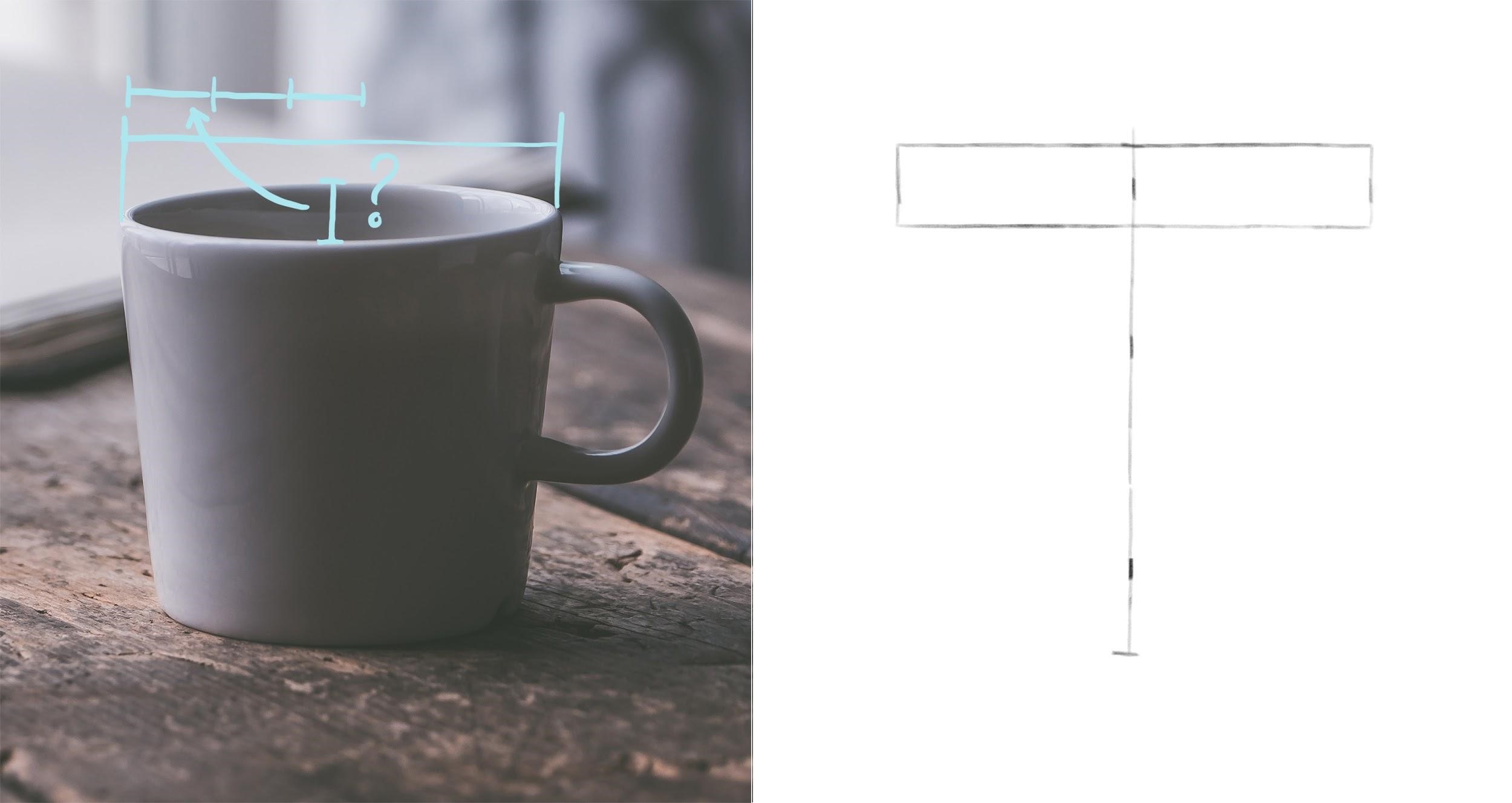
Шаг 3. Проведем горизонтальную ось и впишем эллипс в прямоугольник. Затем найдем ширину нижней части кружки, сравнив ее с шириной верха. Высоту нижнего эллипса мы найдем, измерив расстояние по вертикали от самой нижней отметки кружки до нижней отметки ее бока (до точки, через которую пройдет горизонтальная ось этого эллипса). Найденное расстояние – это половина искомой высоты. Удвоим его и отложим от самой нижней точки кружки. Здесь важно не запутаться: в данном случае ось надо провести через нижнюю точку бока кружки, а не через низ самой кружки. Иначе пропорции нарушатся. Зная высоту нижнего эллипса, проверим, соблюдается ли принцип их постепенного раскрытия по мере удаления от уровня глаз. Верхний эллипс расположен ближе к уровню наших глаз, чем нижний, поэтому должен быть уже. Найдем, сколько раз высота нижнего овала помещается в его ширине – около четырех раз. Для верхнего овала было соотношение примерно 5 к 1. Таким образом нижний овал шире, то есть раскрыт в большей степени. Принцип соблюдается.

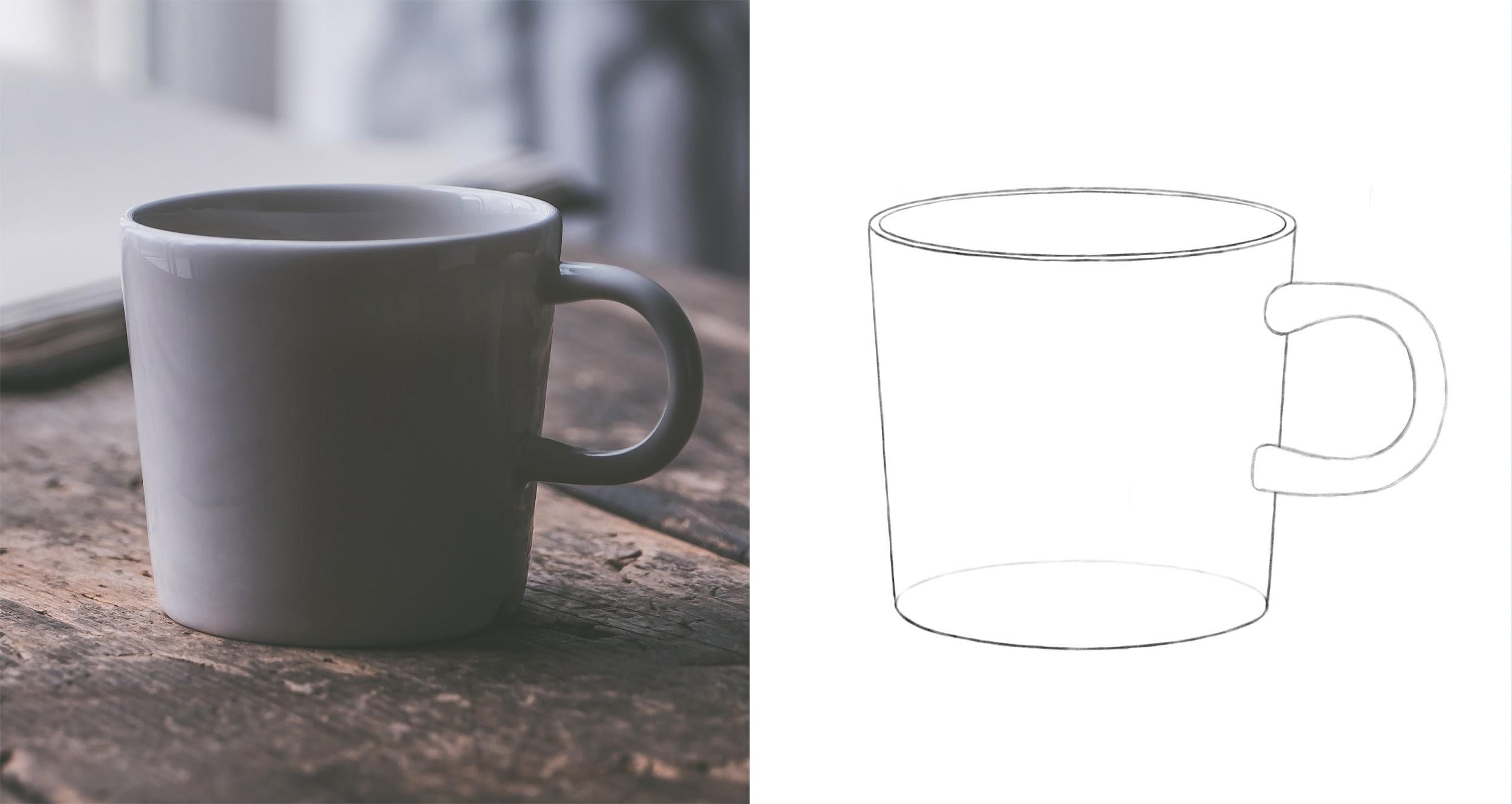
Шаг 4. Рисуем стенки кружки, соединяя боковые вершины верхнего и нижнего эллипсов. Для большей объемности покажем толщину стенки. Нарисуем второй овал внутри верхнего. При этом учитываем, что из-за перспективного искажения толщина стенок выглядит не одинаковой. Передняя и дальняя стенки визуально сужаются сильнее боковых примерно в два раза. Отметим вершины внутреннего овала на некотором расстоянии от вершин первого овала. Делаем этот отступ чуть больше для боковых вершин. Ставим отметки симметрично относительно вертикальной и горизонтальной осей. Нарисуем новый эллипс через эти вершины.

Шаг 5. Найдем расположение ручки и ее общие пропорции, а затем схематично наметим основные отрезки, формирующие ее контур. Их наклоны определяем методом визирования (а где-то — на глаз).

Шаг 6. Уточним контур ручки, сделаем его более плавным. По необходимости подправим очертания кружки. Смягчим немного ластиком линии построения. Выделим более сильным нажимом на карандаш контуры, расположенные ближе к нам. Кружка готова!

Рисуем вазу

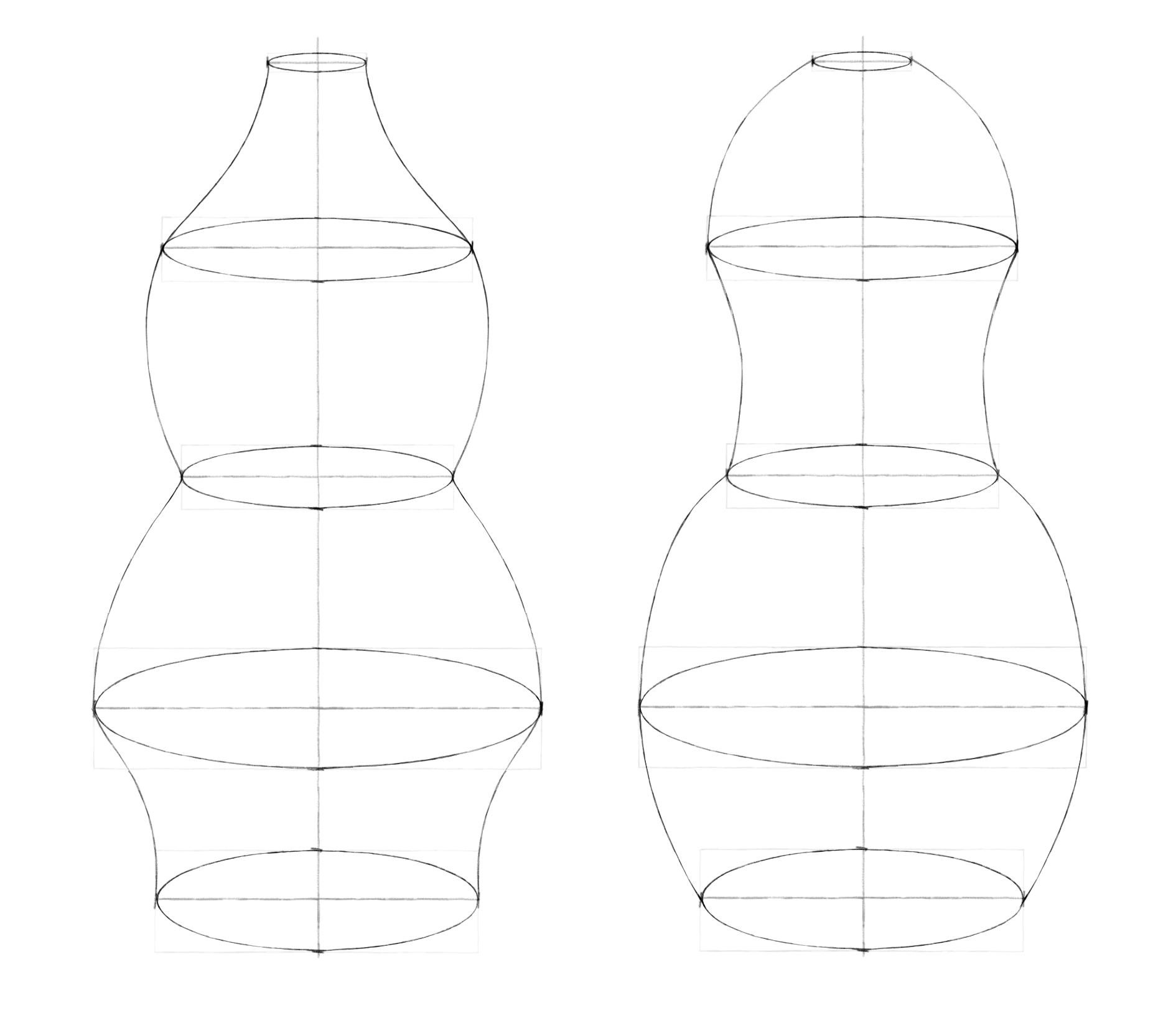
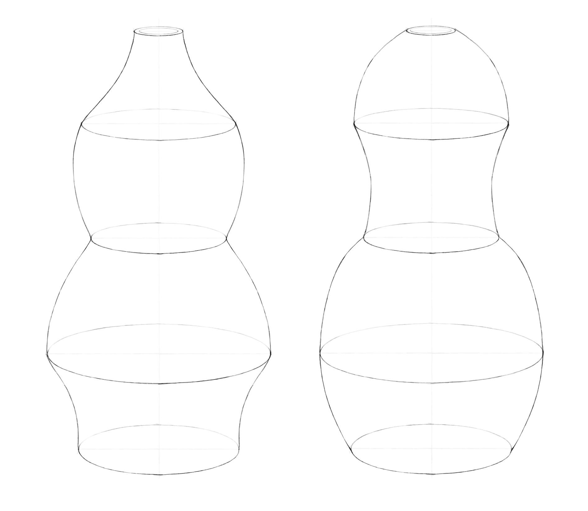
В этом упражнении поработаем с воображением. Придумаем свою вазу и потренируемся рисовать эллипсы.

В прошлом задании для построения кружки было достаточно нарисовать два эллипса. Две ключевые окружности (верхняя и нижняя) определяли ее форму. Диаметр кружки равномерно уменьшался от верха к низу. А, например, форма вазы из рисунка ниже зависит от четырех окружностей (причем верхняя находится на уровне глаз, поэтому превратилась в линию).

Перейдем к рисованию. И помним важный принцип: чем дальше эллипс от уровня глаз, тем более он раскрыт.

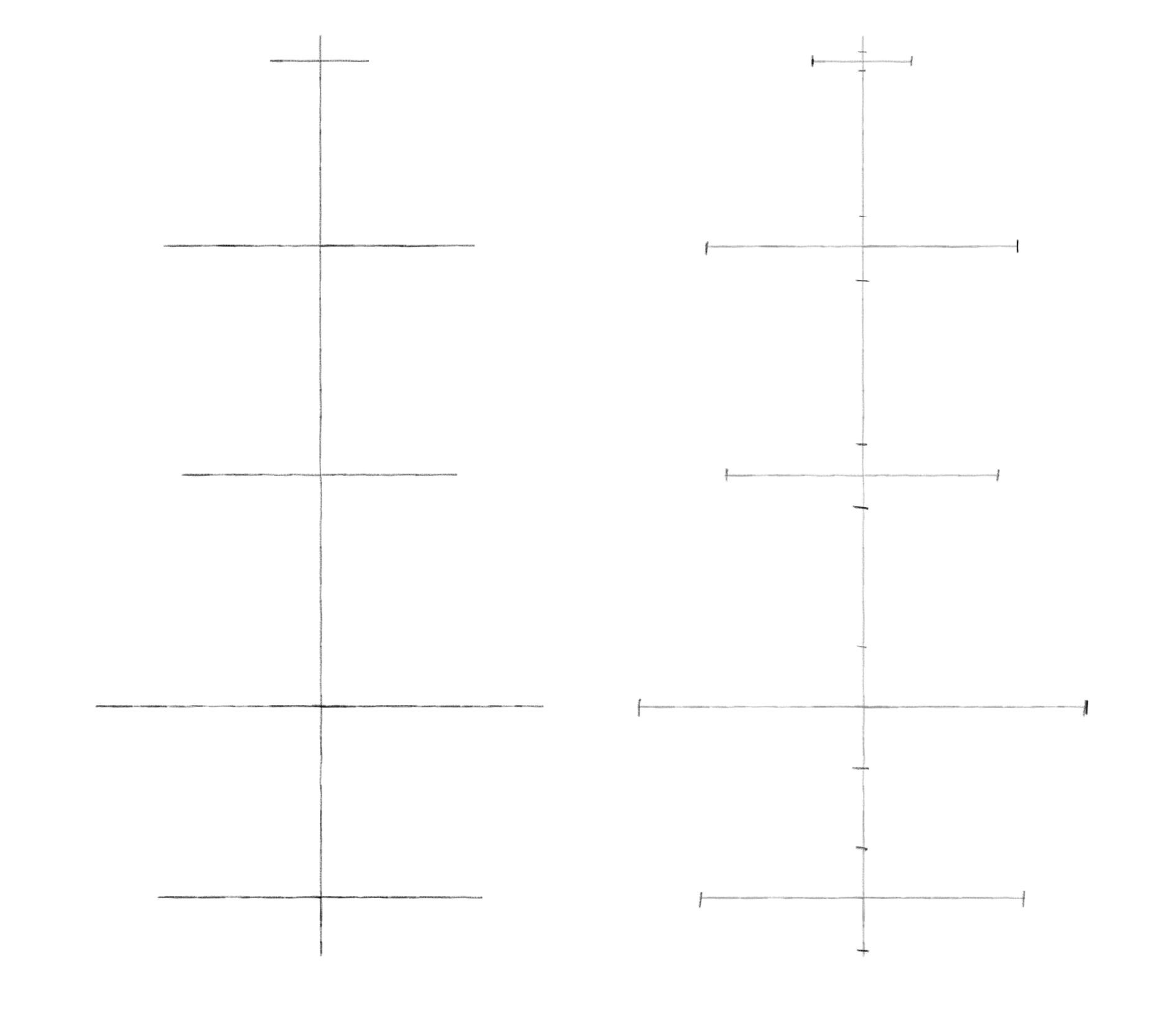
Шаг 1. Проведем вертикальную ось. От нее симметрично отложим горизонтальные оси будущих эллипсов. Длину вертикальной и горизонтальных осей, а также количество эллипсов и расстояние между ними выбирайте сами.

Шаг 2. Обозначим боковые вершины эллипсов симметрично относительно вертикальной оси. Теперь перейдем к обозначению верхних и нижних вершин. И здесь пользуемся принципом постепенного раскрытия эллипсов по мере удаления от линии горизонта. Например, здесь мы рисовали вазу, расположенную в целом ниже уровня глаз. Для первого эллипса взяли высоту, примерно в пять раз меньше ширины. Измеряли это карандашом. Для последующих эллипсов постепенно увеличивали степень раскрытия. Так высота среднего эллипса укладывается в ширине примерно четыре раза, а для самого нижнего – примерно три раза. Чем ближе друг к другу эллипсы, тем ближе они по степени раскрытия. Чем дальше – тем больше разница. Намечая вершины, нижнюю половинку (ближнюю) делаем чуть-чуть больше верхней (дальней).

Шаг 3. Через вершины легкими линиями рисуем прямоугольники. А затем вписываем в них эллипсы.

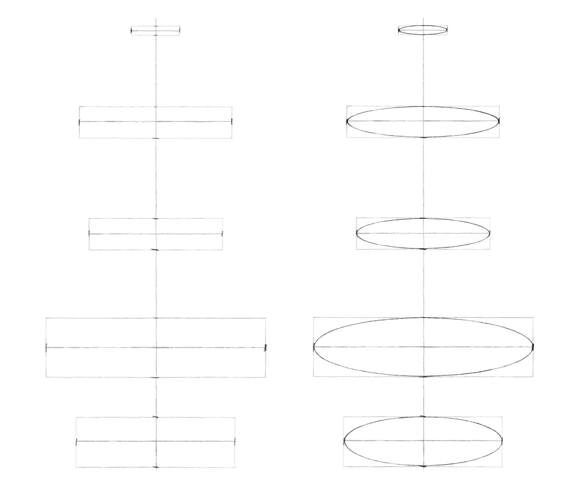
Шаг 4. Теперь самое интересное: надо соединить боковые вершины эллипсов линиями. Вам решать, какими они будут, прямыми или округлыми, вогнутыми или выпуклыми. Можно сделать пару вариантов. Постарайтесь наиболее симметрично повторить форму внешнего контура для двух половинок вазы. Чтобы проверить симметрию, пробуйте перевернуть работу вверх ногами. Взглянув на предмет по-новому, проще увидеть расхождения.

Шаг 5. Так же, как мы делали для кружки, здесь можно показать толщину стенки. Нарисуем внутри верхнего эллипса еще один поменьше, предварительно наметив его вершины. Смягчим ластиком оси и дальние половинки эллипсов. Можно чуть высветлить те эллипсы, в которых изменение формы вазы более плавное. Рисунок готов!

Проверьте свои знания

Если вы хотите проверить свои знания по теме данного урока, можете пройти небольшой тест, состоящий из нескольких вопросов. В каждом вопросе правильным может быть только 1 вариант. После выбора вами одного из вариантов, система автоматически переходит к следующему вопросу. На получаемые вами баллы влияет правильность ваших ответов и затраченное на прохождение время. Обратите внимание, что вопросы каждый раз разные, а варианты перемешиваются.

Напоминаем, что для полноценной работы сайта вам необходимо включить cookies, javascript и iframe. Если вы ввидите это сообщение в течение долгого времени, значит настройки вашего браузера не позволяют нашему порталу полноценно работать.

источники:

Построение овала

http://4brain.ru/draw/okruzhnost-v-vperspective.php

Источник

Not to be confused with eclipse.

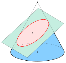
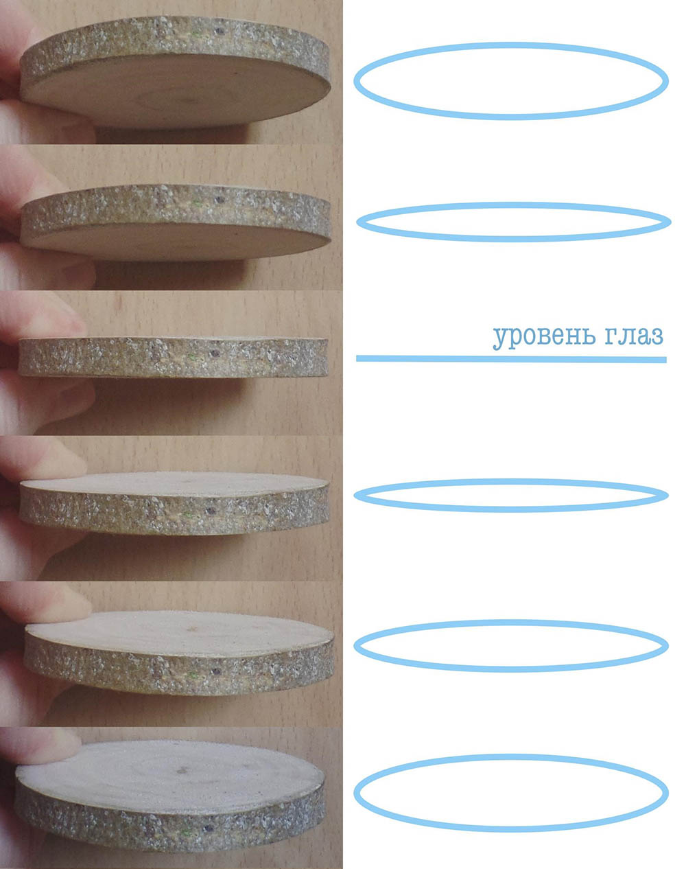
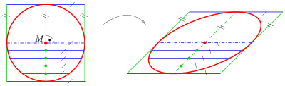
An ellipse (red) obtained as the intersection of a cone with an inclined plane.

Ellipses: examples with increasing eccentricity

In mathematics, an ellipse is a plane curve surrounding two focal points, such that for all points on the curve, the sum of the two distances to the focal points is a constant. It generalizes a circle, which is the special type of ellipse in which the two focal points are the same. The elongation of an ellipse is measured by its eccentricity , a number ranging from e=0 (the limiting case of a circle) to e=1 (the limiting case of infinite elongation, no longer an ellipse but a parabola).

An ellipse has a simple algebraic solution for its area, but only approximations for its perimeter (also known as circumference), for which integration is required to obtain an exact solution.

Analytically, the equation of a standard ellipse centered at the origin with width and height is:

${displaystyle {frac {x^{2}}{a^{2}}}+{frac {y^{2}}{b^{2}}}=1.}$

Assuming a ge b , the foci are for ${textstyle c={sqrt {a^{2}-b^{2}}}}$ . The standard parametric equation is:

{displaystyle (x,y)=(acos(t),bsin(t))quad {text{for}}quad 0leq tleq 2pi .}

Ellipses are the closed type of conic section: a plane curve tracing the intersection of a cone with a plane (see figure). Ellipses have many similarities with the other two forms of conic sections, parabolas and hyperbolas, both of which are open and unbounded. An angled cross section of a cylinder is also an ellipse.

An ellipse may also be defined in terms of one focal point and a line outside the ellipse called the directrix: for all points on the ellipse, the ratio between the distance to the focus and the distance to the directrix is a constant. This constant ratio is the above-mentioned eccentricity:

${displaystyle e={frac {c}{a}}={sqrt {1-{frac {b^{2}}{a^{2}}}}}.}$

Ellipses are common in physics, astronomy and engineering. For example, the orbit of each planet in the Solar System is approximately an ellipse with the Sun at one focus point (more precisely, the focus is the barycenter of the Sun–planet pair). The same is true for moons orbiting planets and all other systems of two astronomical bodies. The shapes of planets and stars are often well described by ellipsoids. A circle viewed from a side angle looks like an ellipse: that is, the ellipse is the image of a circle under parallel or perspective projection. The ellipse is also the simplest Lissajous figure formed when the horizontal and vertical motions are sinusoids with the same frequency: a similar effect leads to elliptical polarization of light in optics.

The name, ἔλλειψις (élleipsis, «omission»), was given by Apollonius of Perga in his Conics.

Definition as locus of points[edit]

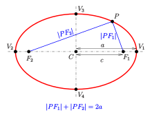
Ellipse: definition by sum of distances to foci

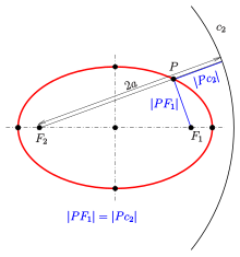
Ellipse: definition by focus and circular directrix

An ellipse can be defined geometrically as a set or locus of points in the Euclidean plane:

Given two fixed points $F_{1},F_{2}$

called the foci and a distance

which is greater than the distance between the foci, the ellipse is the set of points

such that the sum of the distances ${displaystyle |PF_{1}|, |PF_{2}|}$

is equal to

: ${displaystyle E=left{Pin mathbb {R} ^{2},mid ,|PF_{2}|+|PF_{1}|=2aright} .}$

The midpoint of the line segment joining the foci is called the center of the ellipse. The line through the foci is called the major axis, and the line perpendicular to it through the center is the minor axis. The major axis intersects the ellipse at two vertices ${displaystyle V_{1},V_{2}}$ , which have distance to the center. The distance of the foci to the center is called the focal distance or linear eccentricity. The quotient ${displaystyle e={tfrac {c}{a}}}$ is the eccentricity.

The case ${displaystyle F_{1}=F_{2}}$ yields a circle and is included as a special type of ellipse.

The equation ${displaystyle |PF_{2}|+|PF_{1}|=2a}$ can be viewed in a different way (see figure):

If $c_{2}$

is the circle with center $F_{2}$

and radius

, then the distance of a point

to the circle $c_{2}$

equals the distance to the focus $F_{1}$

${displaystyle |PF_{1}|=|Pc_{2}|.}$

$c_{2}$ is called the circular directrix (related to focus $F_{2}$ ) of the ellipse.^[1]^[2] This property should not be confused with the definition of an ellipse using a directrix line below.

Using Dandelin spheres, one can prove that any section of a cone with a plane is an ellipse, assuming the plane does not contain the apex and has slope less than that of the lines on the cone.

In Cartesian coordinates[edit]

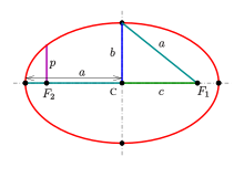
Shape parameters:

a: semi-major axis,
b: semi-minor axis,
c: linear eccentricity,
p: semi-latus rectum (usually ).

Standard equation[edit]

The standard form of an ellipse in Cartesian coordinates assumes that the origin is the center of the ellipse, the x-axis is the major axis, and:

the foci are the points ${displaystyle F_{1}=(c,,0), F_{2}=(-c,,0)}$

the major points are ${displaystyle V_{1}=(a,,0), V_{2}=(-a,,0)}$

For an arbitrary point (x,y) the distance to the focus (c,0) is
${textstyle {sqrt {(x-c)^{2}+y^{2}}}}$ and to the other focus ${textstyle {sqrt {(x+c)^{2}+y^{2}}}}$ . Hence the point is on the ellipse whenever:

${displaystyle {sqrt {(x-c)^{2}+y^{2}}}+{sqrt {(x+c)^{2}+y^{2}}}=2a .}$

Removing the radicals by suitable squarings and using ${displaystyle b^{2}=a^{2}-c^{2}}$ (see diagram) produces the standard equation of the ellipse:^[3]

${displaystyle {frac {x^{2}}{a^{2}}}+{frac {y^{2}}{b^{2}}}=1,}$

or, solved for y:

${displaystyle y=pm {frac {b}{a}}{sqrt {a^{2}-x^{2}}}=pm {sqrt {left(a^{2}-x^{2}right)left(1-e^{2}right)}}.}$

The width and height parameters are called the semi-major and semi-minor axes. The top and bottom points ${displaystyle V_{3}=(0,,b),;V_{4}=(0,,-b)}$ are the co-vertices. The distances from a point on the ellipse to the left and right foci are and .

It follows from the equation that the ellipse is symmetric with respect to the coordinate axes and hence with respect to the origin.

Parameters[edit]

Principal axes[edit]

Throughout this article, the semi-major and semi-minor axes are denoted and , respectively, i.e.

In principle, the canonical ellipse equation ${displaystyle {tfrac {x^{2}}{a^{2}}}+{tfrac {y^{2}}{b^{2}}}=1}$ may have a<b (and hence the ellipse would be taller than it is wide). This form can be converted to the standard form by transposing the variable names and and the parameter names and

Linear eccentricity[edit]

This is the distance from the center to a focus: ${displaystyle c={sqrt {a^{2}-b^{2}}}}$ .

Eccentricity[edit]

The eccentricity can be expressed as:

${displaystyle e={frac {c}{a}}={sqrt {1-left({frac {b}{a}}right)^{2}}},}$

assuming An ellipse with equal axes ( a=b ) has zero eccentricity, and is a circle.

Semi-latus rectum[edit]

The length of the chord through one focus, perpendicular to the major axis, is called the latus rectum. One half of it is the semi-latus rectum ell . A calculation shows:

${displaystyle ell ={frac {b^{2}}{a}}=aleft(1-e^{2}right).}$

^[4]

The semi-latus rectum ell is equal to the radius of curvature at the vertices (see section curvature).

Tangent[edit]

An arbitrary line intersects an ellipse at 0, 1, or 2 points, respectively called an exterior line, tangent and secant. Through any point of an ellipse there is a unique tangent. The tangent at a point ${displaystyle (x_{1},,y_{1})}$ of the ellipse ${displaystyle {tfrac {x^{2}}{a^{2}}}+{tfrac {y^{2}}{b^{2}}}=1}$ has the coordinate equation:

${displaystyle {frac {x_{1}}{a^{2}}}x+{frac {y_{1}}{b^{2}}}y=1.}$

A vector parametric equation of the tangent is:

${displaystyle {vec {x}}={begin{pmatrix}x_{1}\y_{1}end{pmatrix}}+s{begin{pmatrix};!-y_{1}a^{2}\; x_{1}b^{2}end{pmatrix}} }$

with

Proof:
Let ${displaystyle (x_{1},,y_{1})}$ be a point on an ellipse and ${textstyle {vec {x}}={begin{pmatrix}x_{1}\y_{1}end{pmatrix}}+s{begin{pmatrix}u\vend{pmatrix}}}$ be the equation of any line containing ${displaystyle (x_{1},,y_{1})}$ . Inserting the line’s equation into the ellipse equation and respecting ${displaystyle {frac {x_{1}^{2}}{a^{2}}}+{frac {y_{1}^{2}}{b^{2}}}=1}$ yields:

${displaystyle {frac {left(x_{1}+suright)^{2}}{a^{2}}}+{frac {left(y_{1}+svright)^{2}}{b^{2}}}=1 quad Longrightarrow quad 2sleft({frac {x_{1}u}{a^{2}}}+{frac {y_{1}v}{b^{2}}}right)+s^{2}left({frac {u^{2}}{a^{2}}}+{frac {v^{2}}{b^{2}}}right)=0 .}$

There are then cases:

${displaystyle {frac {x_{1}}{a^{2}}}u+{frac {y_{1}}{b^{2}}}v=0.}$ Then line and the ellipse have only point ${displaystyle (x_{1},,y_{1})}$ in common, and is a tangent. The tangent direction has perpendicular vector ${displaystyle {begin{pmatrix}{frac {x_{1}}{a^{2}}}&{frac {y_{1}}{b^{2}}}end{pmatrix}}}$ , so the tangent line has equation ${textstyle {frac {x_{1}}{a^{2}}}x+{tfrac {y_{1}}{b^{2}}}y=k}$ for some . Because ${displaystyle (x_{1},,y_{1})}$ is on the tangent and the ellipse, one obtains .
${displaystyle {frac {x_{1}}{a^{2}}}u+{frac {y_{1}}{b^{2}}}vneq 0.}$ Then line has a second point in common with the ellipse, and is a secant.

Using (1) one finds that ${displaystyle {begin{pmatrix}-y_{1}a^{2}&x_{1}b^{2}end{pmatrix}}}$ is a tangent vector at point ${displaystyle (x_{1},,y_{1})}$ , which proves the vector equation.

If $(x_{1},y_{1})$ and (u,v) are two points of the ellipse such that ${textstyle {frac {x_{1}u}{a^{2}}}+{tfrac {y_{1}v}{b^{2}}}=0}$ , then the points lie on two conjugate diameters (see below). (If a=b , the ellipse is a circle and «conjugate» means «orthogonal».)

Shifted ellipse[edit]

If the standard ellipse is shifted to have center ${displaystyle left(x_{circ },,y_{circ }right)}$ , its equation is

${displaystyle {frac {left(x-x_{circ }right)^{2}}{a^{2}}}+{frac {left(y-y_{circ }right)^{2}}{b^{2}}}=1 .}$

The axes are still parallel to the x- and y-axes.

General ellipse[edit]

In analytic geometry, the ellipse is defined as a quadric: the set of points of the Cartesian plane that, in non-degenerate cases, satisfy the implicit equation^[5]^[6]

${displaystyle AX^{2}+BXY+CY^{2}+DX+EY+F=0}$

provided $B^{2}-4AC<0.$

To distinguish the degenerate cases from the non-degenerate case, let ∆ be the determinant

${displaystyle Delta ={begin{vmatrix}A&{frac {1}{2}}B&{frac {1}{2}}D\{frac {1}{2}}B&C&{frac {1}{2}}E\{frac {1}{2}}D&{frac {1}{2}}E&Fend{vmatrix}}=left(AC-{tfrac {1}{4}}B^{2}right)F+{tfrac {1}{4}}BED-{tfrac {1}{4}}CD^{2}-{tfrac {1}{4}}AE^{2}.}$

Then the ellipse is a non-degenerate real ellipse if and only if C∆ < 0. If C∆ > 0, we have an imaginary ellipse, and if ∆ = 0, we have a point ellipse.^[7]^: p.63

The general equation’s coefficients can be obtained from known semi-major axis , semi-minor axis , center coordinates ${displaystyle left(x_{circ },,y_{circ }right)}$ , and rotation angle theta (the angle from the positive horizontal axis to the ellipse’s major axis) using the formulae:

${displaystyle {begin{aligned}A&=a^{2}sin ^{2}theta +b^{2}cos ^{2}theta \[3mu]B&=2left(b^{2}-a^{2}right)sin theta cos theta \[3mu]C&=a^{2}cos ^{2}theta +b^{2}sin ^{2}theta \[3mu]D&=-2Ax_{circ }-By_{circ }\[3mu]E&=-Bx_{circ }-2Cy_{circ }\[3mu]F&=Ax_{circ }^{2}+Bx_{circ }y_{circ }+Cy_{circ }^{2}-a^{2}b^{2}.end{aligned}}}$

These expressions can be derived from the canonical equation

${frac {x^{2}}{a^{2}}}+{frac {y^{2}}{b^{2}}}=1$

by an affine transformation of the coordinates :

${displaystyle {begin{aligned}x&=left(X-x_{circ }right)cos theta +left(Y-y_{circ }right)sin theta \y&=-left(X-x_{circ }right)sin theta +left(Y-y_{circ }right)cos theta .end{aligned}}}$

Conversely, the canonical form parameters can be obtained from the general form coefficients by the equations:^{[citation needed]}

${displaystyle {begin{aligned}a,b&={frac {-{sqrt {2{big (}AE^{2}+CD^{2}-BDE+(B^{2}-4AC)F{big )}{big (}(A+C)pm {sqrt {(A-C)^{2}+B^{2}}}{big )}}}}{B^{2}-4AC}}\x_{circ }&={frac {2CD-BE}{B^{2}-4AC}}\[5mu]y_{circ }&={frac {2AE-BD}{B^{2}-4AC}}\[5mu]theta &={begin{cases}operatorname {arccot} {dfrac {C-A-{sqrt {(A-C)^{2}+B^{2}}}}{B}}&{text{for }}Bneq 0\[5mu]0&{text{for }}B=0, A<C\[10mu]90^{circ }&{text{for }}B=0, A>C\end{cases}}end{aligned}}}$

Parametric representation[edit]

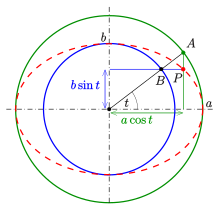
The construction of points based on the parametric equation and the interpretation of parameter t, which is due to de la Hire

Ellipse points calculated by the rational representation with equal spaced parameters ().

Standard parametric representation[edit]

Using trigonometric functions, a parametric representation of the standard ellipse ${tfrac {x^{2}}{a^{2}}}+{tfrac {y^{2}}{b^{2}}}=1$ is:

{displaystyle (x,,y)=(acos t,,bsin t), 0leq t<2pi .}

The parameter t (called the eccentric anomaly in astronomy) is not the angle of with the x-axis, but has a geometric meaning due to Philippe de La Hire (see Drawing ellipses below).^[8]

Rational representation[edit]

With the substitution ${textstyle u=tan left({frac {t}{2}}right)}$ and trigonometric formulae one obtains

${displaystyle cos t={frac {1-u^{2}}{1+u^{2}}} ,quad sin t={frac {2u}{1+u^{2}}}}$

and the rational parametric equation of an ellipse

${displaystyle {begin{aligned}x(u)&=a{frac {1-u^{2}}{1+u^{2}}}\[10mu]y(u)&=b{frac {2u}{1+u^{2}}}end{aligned}};,quad -infty <u<infty ;,}$

which covers any point of the ellipse ${displaystyle {tfrac {x^{2}}{a^{2}}}+{tfrac {y^{2}}{b^{2}}}=1}$ except the left vertex .

For this formula represents the right upper quarter of the ellipse moving counter-clockwise with increasing The left vertex is the limit ${textstyle lim _{uto pm infty }(x(u),,y(u))=(-a,,0);.}$

Alternately, if the parameter is considered to be a point on the real projective line , then the corresponding rational parametrization is

${displaystyle [u:v]mapsto left(a{frac {v^{2}-u^{2}}{v^{2}+u^{2}}},b{frac {2uv}{v^{2}+u^{2}}}right).}$

Then

Rational representations of conic sections are commonly used in computer-aided design (see Bezier curve).

Tangent slope as parameter[edit]

A parametric representation, which uses the slope of the tangent at a point of the ellipse
can be obtained from the derivative of the standard representation ${displaystyle {vec {x}}(t)=(acos t,,bsin t)^{mathsf {T}}}$ :

${displaystyle {vec {x}}'(t)=(-asin t,,bcos t)^{mathsf {T}}quad rightarrow quad m=-{frac {b}{a}}cot tquad rightarrow quad cot t=-{frac {ma}{b}}.}$

With help of trigonometric formulae one obtains:

${displaystyle cos t={frac {cot t}{pm {sqrt {1+cot ^{2}t}}}}={frac {-ma}{pm {sqrt {m^{2}a^{2}+b^{2}}}}} ,quad quad sin t={frac {1}{pm {sqrt {1+cot ^{2}t}}}}={frac {b}{pm {sqrt {m^{2}a^{2}+b^{2}}}}}.}$

Replacing and sin t of the standard representation yields:

${displaystyle {vec {c}}_{pm }(m)=left(-{frac {ma^{2}}{pm {sqrt {m^{2}a^{2}+b^{2}}}}},;{frac {b^{2}}{pm {sqrt {m^{2}a^{2}+b^{2}}}}}right),,min mathbb {R} .}$

Here is the slope of the tangent at the corresponding ellipse point, ${displaystyle {vec {c}}_{+}}$ is the upper and ${displaystyle {vec {c}}_{-}}$ the lower half of the ellipse. The vertices, having vertical tangents, are not covered by the representation.

The equation of the tangent at point ${vec c}_{pm }(m)$ has the form . The still unknown can be determined by inserting the coordinates of the corresponding ellipse point ${vec c}_{pm }(m)$ :

${displaystyle y=mxpm {sqrt {m^{2}a^{2}+b^{2}}};.}$

This description of the tangents of an ellipse is an essential tool for the determination of the orthoptic of an ellipse. The orthoptic article contains another proof, without differential calculus and trigonometric formulae.

General ellipse[edit]

Ellipse as an affine image of the unit circle

Another definition of an ellipse uses affine transformations:

Any ellipse is an affine image of the unit circle with equation

Parametric representation

An affine transformation of the Euclidean plane has the form ${displaystyle {vec {x}}mapsto {vec {f}}!_{0}+A{vec {x}}}$ , where is a regular matrix (with non-zero determinant) and ${displaystyle {vec {f}}!_{0}}$ is an arbitrary vector. If ${displaystyle {vec {f}}!_{1},{vec {f}}!_{2}}$ are the column vectors of the matrix , the unit circle , , is mapped onto the ellipse:

${displaystyle {vec {x}}={vec {p}}(t)={vec {f}}!_{0}+{vec {f}}!_{1}cos t+{vec {f}}!_{2}sin t .}$

Here ${displaystyle {vec {f}}!_{0}}$ is the center and ${displaystyle {vec {f}}!_{1},;{vec {f}}!_{2}}$ are the directions of two conjugate diameters, in general not perpendicular.

Vertices

The four vertices of the ellipse are ${displaystyle {vec {p}}(t_{0}),;{vec {p}}left(t_{0}pm {tfrac {pi }{2}}right),;{vec {p}}left(t_{0}+pi right)}$ , for a parameter $t=t_{0}$ defined by:

${displaystyle cot(2t_{0})={frac {{vec {f}}!_{1}^{,2}-{vec {f}}!_{2}^{,2}}{2{vec {f}}!_{1}cdot {vec {f}}!_{2}}}.}$

(If ${displaystyle {vec {f}}!_{1}cdot {vec {f}}!_{2}=0}$ , then $t_{0}=0$ .) This is derived as follows. The tangent vector at point is:

${displaystyle {vec {p}},'(t)=-{vec {f}}!_{1}sin t+{vec {f}}!_{2}cos t .}$

At a vertex parameter $t=t_{0}$ , the tangent is perpendicular to the major/minor axes, so:

${displaystyle 0={vec {p}}'(t)cdot left({vec {p}}(t)-{vec {f}}!_{0}right)=left(-{vec {f}}!_{1}sin t+{vec {f}}!_{2}cos tright)cdot left({vec {f}}!_{1}cos t+{vec {f}}!_{2}sin tright).}$

Expanding and applying the identities ${displaystyle ;cos ^{2}t-sin ^{2}t=cos 2t, 2sin tcos t=sin 2t;}$ gives the equation for ${displaystyle t=t_{0};.}$

Area

From Apollonios theorem (see below) one obtains:
The area of an ellipse ${displaystyle ;{vec {x}}={vec {f}}_{0}+{vec {f}}_{1}cos t+{vec {f}}_{2}sin t;}$ is

${displaystyle A=pi |det({vec {f}}_{1},{vec {f}}_{2})| .}$

Semiaxes

With the abbreviations
${displaystyle ;M={vec {f}}_{1}^{2}+{vec {f}}_{2}^{2}, N=left|det({vec {f}}_{1},{vec {f}}_{2})right|}$ the statements of Apollonios’s theorem can be written as:

${displaystyle a^{2}+b^{2}=M,quad ab=N .}$

Solving this nonlinear system for a,b yields the semiaxes:

${displaystyle a={frac {1}{2}}({sqrt {M+2N}}+{sqrt {M-2N}})}$

${displaystyle b={frac {1}{2}}({sqrt {M+2N}}-{sqrt {M-2N}}) .}$

Implicit representation

Solving the parametric representation for by Cramer’s rule and using ${displaystyle ;cos ^{2}t+sin ^{2}t-1=0;}$ , one obtains the implicit representation

${displaystyle det({vec {x}}!-!{vec {f}}!_{0},{vec {f}}!_{2})^{2}+det({vec {f}}!_{1},{vec {x}}!-!{vec {f}}!_{0})^{2}-det({vec {f}}!_{1},{vec {f}}!_{2})^{2}=0}$

Conversely: If the equation

${displaystyle x^{2}+2cxy+d^{2}y^{2}-e^{2}=0 ,}$

with ${displaystyle ;d^{2}-c^{2}>0;,}$

of an ellipse centered at the origin is given, then the two vectors

${displaystyle {vec {f}}_{1}={e choose 0},quad {vec {f}}_{2}={frac {e}{sqrt {d^{2}-c^{2}}}}{-c choose 1} }$

point to two conjugate points and the tools developed above are applicable.

Example: For the ellipse with equation ${displaystyle ;x^{2}+2xy+3y^{2}-1=0;}$ the vectors are

${displaystyle {vec {f}}_{1}={1 choose 0},quad {vec {f}}_{2}={frac {1}{sqrt {2}}}{-1 choose 1}}$

Whirls: nested, scaled and rotated ellipses. The spiral is not drawn: we see it as the locus of points where the ellipses are especially close to each other.

Rotated Standard ellipse

For ${displaystyle {vec {f}}_{0}={0 choose 0},;{vec {f}}_{1}=a{cos theta choose sin theta },;{vec {f}}_{2}=b{-sin theta choose ;cos theta }}$ one obtains a parametric representation of the standard ellipse rotated by angle theta :

${displaystyle x=x_{theta }(t)=acos theta cos t-bsin theta sin t ,}$

${displaystyle y=y_{theta }(t)=asin theta cos t+bcos theta sin t .}$

Ellipse in space

The definition of an ellipse in this section gives a parametric representation of an arbitrary ellipse, even in space, if one allows ${displaystyle {vec {f}}!_{0},{vec {f}}!_{1},{vec {f}}!_{2}}$ to be vectors in space.

Polar forms[edit]

Polar form relative to center[edit]

Polar coordinates centered at the center.

In polar coordinates, with the origin at the center of the ellipse and with the angular coordinate theta measured from the major axis, the ellipse’s equation is^[7]^{: p. 75}

${displaystyle r(theta )={frac {ab}{sqrt {(bcos theta )^{2}+(asin theta )^{2}}}}={frac {b}{sqrt {1-(ecos theta )^{2}}}}}$

where is the eccentricity, not Euler’s number

Polar form relative to focus[edit]

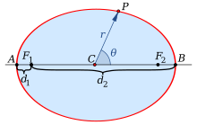
Polar coordinates centered at focus.

If instead we use polar coordinates with the origin at one focus, with the angular coordinate still measured from the major axis, the ellipse’s equation is

${displaystyle r(theta )={frac {a(1-e^{2})}{1pm ecos theta }}}$

where the sign in the denominator is negative if the reference direction points towards the center (as illustrated on the right), and positive if that direction points away from the center.

In the slightly more general case of an ellipse with one focus at the origin and the other focus at angular coordinate phi , the polar form is

${displaystyle r(theta )={frac {a(1-e^{2})}{1-ecos(theta -phi )}}.}$

The angle theta in these formulas is called the true anomaly of the point. The numerator of these formulas is the semi-latus rectum ${displaystyle ell =a(1-e^{2})}$ .

Eccentricity and the directrix property[edit]

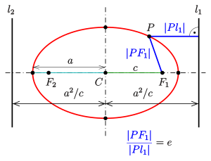
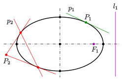
Ellipse: directrix property

Each of the two lines parallel to the minor axis, and at a distance of ${textstyle d={frac {a^{2}}{c}}={frac {a}{e}}}$ from it, is called a directrix of the ellipse (see diagram).

For an arbitrary point

of the ellipse, the quotient of the distance to one focus and to the corresponding directrix (see diagram) is equal to the eccentricity:

${displaystyle {frac {left|PF_{1}right|}{left|Pl_{1}right|}}={frac {left|PF_{2}right|}{left|Pl_{2}right|}}=e={frac {c}{a}} .}$

The proof for the pair ${displaystyle F_{1},l_{1}}$ follows from the fact that ${displaystyle left|PF_{1}right|^{2}=(x-c)^{2}+y^{2}, left|Pl_{1}right|^{2}=left(x-{tfrac {a^{2}}{c}}right)^{2}}$ and ${displaystyle y^{2}=b^{2}-{tfrac {b^{2}}{a^{2}}}x^{2}}$ satisfy the equation

${displaystyle left|PF_{1}right|^{2}-{frac {c^{2}}{a^{2}}}left|Pl_{1}right|^{2}=0 .}$

The second case is proven analogously.

The converse is also true and can be used to define an ellipse (in a manner similar to the definition of a parabola):

For any point

(focus), any line

(directrix) not through

, and any real number

with

the ellipse is the locus of points for which the quotient of the distances to the point and to the line is

that is:

${displaystyle E=left{P left| {frac {|PF|}{|Pl|}}=eright.right}.}$

The extension to e=0 , which is the eccentricity of a circle, is not allowed in this context in the Euclidean plane. However, one may consider the directrix of a circle to be the line at infinity in the projective plane.

(The choice e=1 yields a parabola, and if e>1 , a hyperbola.)

Pencil of conics with a common vertex and common semi-latus rectum

Proof

Let , and assume is a point on the curve.
The directrix has equation ${displaystyle x=-{tfrac {f}{e}}}$ . With , the relation ${displaystyle |PF|^{2}=e^{2}|Pl|^{2}}$ produces the equations

${displaystyle (x-f)^{2}+y^{2}=e^{2}left(x+{frac {f}{e}}right)^{2}=(ex+f)^{2}}$

and ${displaystyle x^{2}left(e^{2}-1right)+2xf(1+e)-y^{2}=0.}$

The substitution yields

${displaystyle x^{2}left(e^{2}-1right)+2px-y^{2}=0.}$

This is the equation of an ellipse (), or a parabola ( e=1 ), or a hyperbola ( e>1 ). All of these non-degenerate conics have, in common, the origin as a vertex (see diagram).

If , introduce new parameters so that ${displaystyle 1-e^{2}={tfrac {b^{2}}{a^{2}}},{text{ and }} p={tfrac {b^{2}}{a}}}$ , and then the equation above becomes

${displaystyle {frac {(x-a)^{2}}{a^{2}}}+{frac {y^{2}}{b^{2}}}=1 ,}$

which is the equation of an ellipse with center , the x-axis as major axis, and
the major/minor semi axis .

Construction of a directrix

Construction of a directrix

Because of ${displaystyle ccdot {tfrac {a^{2}}{c}}=a^{2}}$ point $L_{1}$ of directrix $l_{1}$ (see diagram) and focus $F_{1}$ are inverse with respect to the circle inversion at circle ${displaystyle x^{2}+y^{2}=a^{2}}$ (in diagram green). Hence $L_{1}$ can be constructed as shown in the diagram. Directrix $l_{1}$ is the perpendicular to the main axis at point $L_{1}$ .

General ellipse

If the focus is ${displaystyle F=left(f_{1},,f_{2}right)}$ and the directrix , one obtains the equation

${displaystyle left(x-f_{1}right)^{2}+left(y-f_{2}right)^{2}=e^{2}{frac {left(ux+vy+wright)^{2}}{u^{2}+v^{2}}} .}$

(The right side of the equation uses the Hesse normal form of a line to calculate the distance .)

Focus-to-focus reflection property[edit]

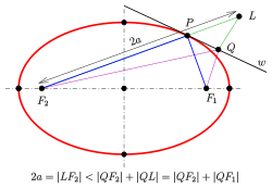
Ellipse: the tangent bisects the supplementary angle of the angle between the lines to the foci.

Rays from one focus reflect off the ellipse to pass through the other focus.

An ellipse possesses the following property:

The normal at a point

bisects the angle between the lines ${displaystyle {overline {PF_{1}}},,{overline {PF_{2}}}}$

Proof

Because the tangent is perpendicular to the normal, the statement is true for the tangent and the supplementary angle of the angle between the lines to the foci (see diagram), too.

Let be the point on the line ${displaystyle {overline {PF_{2}}}}$ with the distance to the focus $F_{2}$ , is the semi-major axis of the ellipse. Let line be the bisector of the supplementary angle to the angle between the lines ${displaystyle {overline {PF_{1}}},,{overline {PF_{2}}}}$ . In order to prove that is the tangent line at point , one checks that any point on line which is different from cannot be on the ellipse. Hence has only point in common with the ellipse and is, therefore, the tangent at point .

From the diagram and the triangle inequality one recognizes that ${displaystyle 2a=left|LF_{2}right|<left|QF_{2}right|+left|QLright|=left|QF_{2}right|+left|QF_{1}right|}$ holds, which means: ${displaystyle left|QF_{2}right|+left|QF_{1}right|>2a}$ . The equality ${displaystyle left|QLright|=left|QF_{1}right|}$ is true from the Angle bisector theorem because ${displaystyle {frac {left|PLright|}{left|PF_{1}right|}}={frac {left|QLright|}{left|QF_{1}right|}}}$ and ${displaystyle left|PLright|=left|PF_{1}right|}$ . But if is a point of the ellipse, the sum should be .

Application

The rays from one focus are reflected by the ellipse to the second focus. This property has optical and acoustic applications similar to the reflective property of a parabola (see whispering gallery).

Conjugate diameters[edit]

Definition of conjugate diameters[edit]

Orthogonal diameters of a circle with a square of tangents, midpoints of parallel chords and an affine image, which is an ellipse with conjugate diameters, a parallelogram of tangents and midpoints of chords.

A circle has the following property:

The midpoints of parallel chords lie on a diameter.

An affine transformation preserves parallelism and midpoints of line segments, so this property is true for any ellipse. (Note that the parallel chords and the diameter are no longer orthogonal.)

Definition

Two diameters ${displaystyle d_{1},,d_{2}}$ of an ellipse are conjugate if the midpoints of chords parallel to $d_{1}$ lie on ${displaystyle d_{2} .}$

From the diagram one finds:

Two diameters ${displaystyle {overline {P_{1}Q_{1}}},,{overline {P_{2}Q_{2}}}}$

of an ellipse are conjugate whenever the tangents at $P_{1}$

and $Q_{1}$

are parallel to ${displaystyle {overline {P_{2}Q_{2}}}}$

Conjugate diameters in an ellipse generalize orthogonal diameters in a circle.

In the parametric equation for a general ellipse given above,

${displaystyle {vec {x}}={vec {p}}(t)={vec {f}}!_{0}+{vec {f}}!_{1}cos t+{vec {f}}!_{2}sin t,}$

any pair of points belong to a diameter, and the pair ${displaystyle {vec {p}}left(t+{tfrac {pi }{2}}right), {vec {p}}left(t-{tfrac {pi }{2}}right)}$ belong to its conjugate diameter.

For the common parametric representation of the ellipse with equation ${tfrac {x^{2}}{a^{2}}}+{tfrac {y^{2}}{b^{2}}}=1$ one gets: The points

${displaystyle (x_{1},y_{1})=(pm acos t,pm bsin t)quad }$

(signs: (+,+) or (-,-) )

${displaystyle (x_{2},y_{2})=({color {red}{mp }}asin t,pm bcos t)quad }$

(signs: (-,+) or (+,-) )

are conjugate and

${displaystyle {frac {x_{1}x_{2}}{a^{2}}}+{frac {y_{1}y_{2}}{b^{2}}}=0 .}$

In case of a circle the last equation collapses to ${displaystyle x_{1}x_{2}+y_{1}y_{2}=0 .}$

Theorem of Apollonios on conjugate diameters[edit]

For the alternative area formula

For an ellipse with semi-axes the following is true:^[9]^[10]

Let ${displaystyle c_{1}}$

and ${displaystyle c_{2}}$

be halves of two conjugate diameters (see diagram) then

${displaystyle c_{1}^{2}+c_{2}^{2}=a^{2}+b^{2}}$ .
The triangle ${displaystyle O,P_{1},P_{2}}$ with sides ${displaystyle c_{1},,c_{2}}$ (see diagram) has the constant area ${textstyle A_{Delta }={frac {1}{2}}ab}$ , which can be expressed by ${displaystyle A_{Delta }={tfrac {1}{2}}c_{2}d_{1}={tfrac {1}{2}}c_{1}c_{2}sin alpha }$ , too. $d_{1}$ is the altitude of point $P_{1}$ and the angle between the half diameters. Hence the area of the ellipse (see section metric properties) can be written as ${displaystyle A_{el}=pi ab=pi c_{2}d_{1}=pi c_{1}c_{2}sin alpha }$ .
The parallelogram of tangents adjacent to the given conjugate diameters has the ${displaystyle {text{Area}}_{12}=4ab .}$

Proof

Let the ellipse be in the canonical form with parametric equation

{displaystyle {vec {p}}(t)=(acos t,,bsin t)}

The two points ${displaystyle {vec {c}}_{1}={vec {p}}(t), {vec {c}}_{2}={vec {p}}left(t+{frac {pi }{2}}right)}$ are on conjugate diameters (see previous section). From trigonometric formulae one obtains ${displaystyle {vec {c}}_{2}=(-asin t,,bcos t)^{mathsf {T}}}$ and

${displaystyle left|{vec {c}}_{1}right|^{2}+left|{vec {c}}_{2}right|^{2}=cdots =a^{2}+b^{2} .}$

The area of the triangle generated by ${displaystyle {vec {c}}_{1},,{vec {c}}_{2}}$ is

${displaystyle A_{Delta }={frac {1}{2}}det left({vec {c}}_{1},,{vec {c}}_{2}right)=cdots ={frac {1}{2}}ab}$

and from the diagram it can be seen that the area of the parallelogram is 8 times that of ${displaystyle A_{Delta }}$ . Hence

${displaystyle {text{Area}}_{12}=4ab .}$

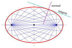
Orthogonal tangents[edit]

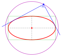
Ellipse with its orthoptic

For the ellipse ${tfrac {x^{2}}{a^{2}}}+{tfrac {y^{2}}{b^{2}}}=1$ the intersection points of orthogonal tangents lie on the circle $x^{2}+y^{2}=a^{2}+b^{2}$ .

This circle is called orthoptic or director circle of the ellipse (not to be confused with the circular directrix defined above).

Drawing ellipses[edit]

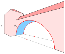
Central projection of circles (gate)

Ellipses appear in descriptive geometry as images (parallel or central projection) of circles. There exist various tools to draw an ellipse. Computers provide the fastest and most accurate method for drawing an ellipse. However, technical tools (ellipsographs) to draw an ellipse without a computer exist. The principle of ellipsographs were known to Greek mathematicians such as Archimedes and Proklos.

If there is no ellipsograph available, one can draw an ellipse using an approximation by the four osculating circles at the vertices.

For any method described below, knowledge of the axes and the semi-axes is necessary (or equivalently: the foci and the semi-major axis).
If this presumption is not fulfilled one has to know at least two conjugate diameters. With help of Rytz’s construction the axes and semi-axes can be retrieved.

de La Hire’s point construction[edit]

The following construction of single points of an ellipse is due to de La Hire.^[11] It is based on the standard parametric representation of an ellipse:

Draw the two circles centered at the center of the ellipse with radii and the axes of the ellipse.
Draw a line through the center, which intersects the two circles at point and , respectively.
Draw a line through that is parallel to the minor axis and a line through that is parallel to the major axis. These lines meet at an ellipse point (see diagram).
Repeat steps (2) and (3) with different lines through the center.

de La Hire’s method
Animation of the method

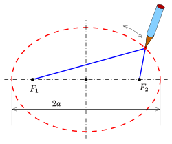
Ellipse: gardener’s method

Pins-and-string method[edit]

The characterization of an ellipse as the locus of points so that sum of the distances to the foci is constant leads to a method of drawing one using two drawing pins, a length of string, and a pencil. In this method, pins are pushed into the paper at two points, which become the ellipse’s foci. A string is tied at each end to the two pins; its length after tying is . The tip of the pencil then traces an ellipse if it is moved while keeping the string taut. Using two pegs and a rope, gardeners use this procedure to outline an elliptical flower bed—thus it is called the gardener’s ellipse.

A similar method for drawing confocal ellipses with a closed string is due to the Irish bishop Charles Graves.

Paper strip methods[edit]

The two following methods rely on the parametric representation (see section parametric representation, above):

This representation can be modeled technically by two simple methods. In both cases center, the axes and semi axes have to be known.

Method 1

The first method starts with

a strip of paper of length a+b

The point, where the semi axes meet is marked by . If the strip slides with both ends on the axes of the desired ellipse, then point traces the ellipse. For the proof one shows that point has the parametric representation , where parameter is the angle of the slope of the paper strip.

A technical realization of the motion of the paper strip can be achieved by a Tusi couple (see animation). The device is able to draw any ellipse with a fixed sum a+b , which is the radius of the large circle. This restriction may be a disadvantage in real life. More flexible is the second paper strip method.

Ellipse construction: paper strip method 1
Ellipses with Tusi couple. Two examples: red and cyan.

A variation of the paper strip method 1 uses the observation that the midpoint of the paper strip is moving on the circle with center (of the ellipse) and radius ${displaystyle {tfrac {a+b}{2}}}$ . Hence, the paperstrip can be cut at point into halves, connected again by a joint at and the sliding end fixed at the center (see diagram). After this operation the movement of the unchanged half of the paperstrip is unchanged.^[12] This variation requires only one sliding shoe.

Variation of the paper strip method 1
Animation of the variation of the paper strip method 1

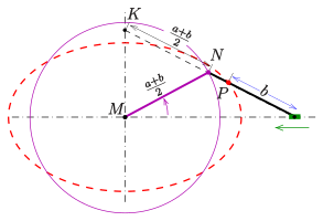
Ellipse construction: paper strip method 2

Method 2

The second method starts with

a strip of paper of length

One marks the point, which divides the strip into two substrips of length and a-b . The strip is positioned onto the axes as described in the diagram. Then the free end of the strip traces an ellipse, while the strip is moved. For the proof, one recognizes that the tracing point can be described parametrically by , where parameter is the angle of slope of the paper strip.

This method is the base for several ellipsographs (see section below).

Similar to the variation of the paper strip method 1 a variation of the paper strip method 2 can be established (see diagram) by cutting the part between the axes into halves.

Variation of the paper strip method 2

Most ellipsograph drafting instruments are based on the second paperstrip method.

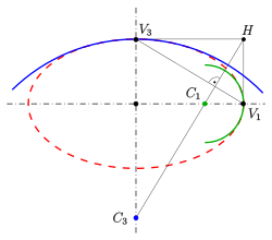
Approximation of an ellipse with osculating circles

Approximation by osculating circles[edit]

From Metric properties below, one obtains:

The diagram shows an easy way to find the centers of curvature ${displaystyle C_{1}=left(a-{tfrac {b^{2}}{a}},0right),,C_{3}=left(0,b-{tfrac {a^{2}}{b}}right)}$ at vertex $V_{1}$ and co-vertex $V_{3}$ , respectively:

mark the auxiliary point and draw the line segment ${displaystyle V_{1}V_{3} ,}$
draw the line through , which is perpendicular to the line ${displaystyle V_{1}V_{3} ,}$
the intersection points of this line with the axes are the centers of the osculating circles.

(proof: simple calculation.)

The centers for the remaining vertices are found by symmetry.

With help of a French curve one draws a curve, which has smooth contact to the osculating circles.

Steiner generation[edit]

Ellipse: Steiner generation

The following method to construct single points of an ellipse relies on the Steiner generation of a conic section:

Given two pencils

of lines at two points

(all lines containing

and

, respectively) and a projective but not perspective mapping

onto

, then the intersection points of corresponding lines form a non-degenerate projective conic section.

For the generation of points of the ellipse ${displaystyle {tfrac {x^{2}}{a^{2}}}+{tfrac {y^{2}}{b^{2}}}=1}$ one uses the pencils at the vertices ${displaystyle V_{1},,V_{2}}$ . Let be an upper co-vertex of the ellipse and .

is the center of the rectangle ${displaystyle V_{1},,V_{2},,B,,A}$ . The side of the rectangle is divided into n equal spaced line segments and this division is projected parallel with the diagonal ${displaystyle AV_{2}}$ as direction onto the line segment ${displaystyle {overline {V_{1}B}}}$ and assign the division as shown in the diagram. The parallel projection together with the reverse of the orientation is part of the projective mapping between the pencils at $V_{1}$ and $V_{2}$ needed. The intersection points of any two related lines ${displaystyle V_{1}B_{i}}$ and ${displaystyle V_{2}A_{i}}$ are points of the uniquely defined ellipse. With help of the points ${displaystyle C_{1},,dotsc }$ the points of the second quarter of the ellipse can be determined. Analogously one obtains the points of the lower half of the ellipse.

Steiner generation can also be defined for hyperbolas and parabolas. It is sometimes called a parallelogram method because one can use other points rather than the vertices, which starts with a parallelogram instead of a rectangle.

As hypotrochoid[edit]

An ellipse (in red) as a special case of the hypotrochoid with R = 2r

The ellipse is a special case of the hypotrochoid when , as shown in the adjacent image. The special case of a moving circle with radius inside a circle with radius is called a Tusi couple.

Inscribed angles and three-point form[edit]

Circles[edit]

Circle: inscribed angle theorem

A circle with equation ${displaystyle left(x-x_{circ }right)^{2}+left(y-y_{circ }right)^{2}=r^{2}}$ is uniquely determined by three points ${displaystyle left(x_{1},y_{1}right),;left(x_{2},,y_{2}right),;left(x_{3},,y_{3}right)}$ not on a line. A simple way to determine the parameters ${displaystyle x_{circ },y_{circ },r}$ uses the inscribed angle theorem for circles:

For four points ${displaystyle P_{i}=left(x_{i},,y_{i}right), i=1,,2,,3,,4,,}$

(see diagram) the following statement is true:

The four points are on a circle if and only if the angles at $P_{3}$

and $P_{4}$

are equal.

Usually one measures inscribed angles by a degree or radian θ, but here the following measurement is more convenient:

In order to measure the angle between two lines with equations ${displaystyle y=m_{1}x+d_{1}, y=m_{2}x+d_{2}, m_{1}neq m_{2},}$

one uses the quotient:

${displaystyle {frac {1+m_{1}m_{2}}{m_{2}-m_{1}}}=cot theta .}$

Inscribed angle theorem for circles[edit]

For four points ${displaystyle P_{i}=left(x_{i},,y_{i}right), i=1,,2,,3,,4,,}$ no three of them on a line, we have the following (see diagram):

The four points are on a circle, if and only if the angles at $P_{3}$

and $P_{4}$

are equal. In terms of the angle measurement above, this means:

${displaystyle {frac {(x_{4}-x_{1})(x_{4}-x_{2})+(y_{4}-y_{1})(y_{4}-y_{2})}{(y_{4}-y_{1})(x_{4}-x_{2})-(y_{4}-y_{2})(x_{4}-x_{1})}}={frac {(x_{3}-x_{1})(x_{3}-x_{2})+(y_{3}-y_{1})(y_{3}-y_{2})}{(y_{3}-y_{1})(x_{3}-x_{2})-(y_{3}-y_{2})(x_{3}-x_{1})}}.}$

At first the measure is available only for chords not parallel to the y-axis, but the final formula works for any chord.

Three-point form of circle equation[edit]

As a consequence, one obtains an equation for the circle determined by three non-colinear points ${displaystyle P_{i}=left(x_{i},,y_{i}right)}$

${displaystyle {frac {({color {red}x}-x_{1})({color {red}x}-x_{2})+({color {red}y}-y_{1})({color {red}y}-y_{2})}{({color {red}y}-y_{1})({color {red}x}-x_{2})-({color {red}y}-y_{2})({color {red}x}-x_{1})}}={frac {(x_{3}-x_{1})(x_{3}-x_{2})+(y_{3}-y_{1})(y_{3}-y_{2})}{(y_{3}-y_{1})(x_{3}-x_{2})-(y_{3}-y_{2})(x_{3}-x_{1})}}.}$

For example, for ${displaystyle P_{1}=(2,,0),;P_{2}=(0,,1),;P_{3}=(0,,0)}$ the three-point equation is:

${displaystyle {frac {(x-2)x+y(y-1)}{yx-(y-1)(x-2)}}=0}$

, which can be rearranged to ${displaystyle (x-1)^{2}+left(y-{tfrac {1}{2}}right)^{2}={tfrac {5}{4}} .}$

Using vectors, dot products and determinants this formula can be arranged more clearly, letting :

${displaystyle {frac {left({color {red}{vec {x}}}-{vec {x}}_{1}right)cdot left({color {red}{vec {x}}}-{vec {x}}_{2}right)}{det left({color {red}{vec {x}}}-{vec {x}}_{1},{color {red}{vec {x}}}-{vec {x}}_{2}right)}}={frac {left({vec {x}}_{3}-{vec {x}}_{1}right)cdot left({vec {x}}_{3}-{vec {x}}_{2}right)}{det left({vec {x}}_{3}-{vec {x}}_{1},{vec {x}}_{3}-{vec {x}}_{2}right)}}.}$

The center of the circle ${displaystyle left(x_{circ },,y_{circ }right)}$ satisfies:

${displaystyle {begin{bmatrix}1&{frac {y_{1}-y_{2}}{x_{1}-x_{2}}}\{frac {x_{1}-x_{3}}{y_{1}-y_{3}}}&1end{bmatrix}}{begin{bmatrix}x_{circ }\y_{circ }end{bmatrix}}={begin{bmatrix}{frac {x_{1}^{2}-x_{2}^{2}+y_{1}^{2}-y_{2}^{2}}{2(x_{1}-x_{2})}}\{frac {y_{1}^{2}-y_{3}^{2}+x_{1}^{2}-x_{3}^{2}}{2(y_{1}-y_{3})}}end{bmatrix}}.}$

The radius is the distance between any of the three points and the center.

${displaystyle r={sqrt {left(x_{1}-x_{circ }right)^{2}+left(y_{1}-y_{circ }right)^{2}}}={sqrt {left(x_{2}-x_{circ }right)^{2}+left(y_{2}-y_{circ }right)^{2}}}={sqrt {left(x_{3}-x_{circ }right)^{2}+left(y_{3}-y_{circ }right)^{2}}}.}$

Ellipses[edit]

This section, we consider the family of ellipses defined by equations ${displaystyle {tfrac {left(x-x_{circ }right)^{2}}{a^{2}}}+{tfrac {left(y-y_{circ }right)^{2}}{b^{2}}}=1}$ with a fixed eccentricity . It is convenient to use the parameter:

${displaystyle {color {blue}q}={frac {a^{2}}{b^{2}}}={frac {1}{1-e^{2}}},}$

and to write the ellipse equation as:

${displaystyle left(x-x_{circ }right)^{2}+{color {blue}q},left(y-y_{circ }right)^{2}=a^{2},}$

where q is fixed and ${displaystyle x_{circ },,y_{circ },,a}$ vary over the real numbers. (Such ellipses have their axes parallel to the coordinate axes: if , the major axis is parallel to the x-axis; if , it is parallel to the y-axis.)

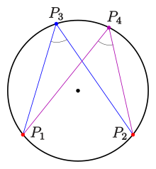
Inscribed angle theorem for an ellipse

Like a circle, such an ellipse is determined by three points not on a line.

For this family of ellipses, one introduces the following q-analog angle measure, which is not a function of the usual angle measure θ:^[13]^[14]

In order to measure an angle between two lines with equations ${displaystyle y=m_{1}x+d_{1}, y=m_{2}x+d_{2}, m_{1}neq m_{2}}$

one uses the quotient:

${displaystyle {frac {1+{color {blue}q};m_{1}m_{2}}{m_{2}-m_{1}}} .}$

Inscribed angle theorem for ellipses[edit]

Given four points ${displaystyle P_{i}=left(x_{i},,y_{i}right), i=1,,2,,3,,4}$

, no three of them on a line (see diagram).

The four points are on an ellipse with equation ${displaystyle (x-x_{circ })^{2}+{color {blue}q},(y-y_{circ })^{2}=a^{2}}$

if and only if the angles at $P_{3}$

and $P_{4}$

are equal in the sense of the measurement above—that is, if

${displaystyle {frac {(x_{4}-x_{1})(x_{4}-x_{2})+{color {blue}q};(y_{4}-y_{1})(y_{4}-y_{2})}{(y_{4}-y_{1})(x_{4}-x_{2})-(y_{4}-y_{2})(x_{4}-x_{1})}}={frac {(x_{3}-x_{1})(x_{3}-x_{2})+{color {blue}q};(y_{3}-y_{1})(y_{3}-y_{2})}{(y_{3}-y_{1})(x_{3}-x_{2})-(y_{3}-y_{2})(x_{3}-x_{1})}} .}$

At first the measure is available only for chords which are not parallel to the y-axis. But the final formula works for any chord. The proof follows from a straightforward calculation. For the direction of proof given that the points are on an ellipse, one can assume that the center of the ellipse is the origin.

Three-point form of ellipse equation[edit]

A consequence, one obtains an equation for the ellipse determined by three non-colinear points ${displaystyle P_{i}=left(x_{i},,y_{i}right)}$

${displaystyle {frac {({color {red}x}-x_{1})({color {red}x}-x_{2})+{color {blue}q};({color {red}y}-y_{1})({color {red}y}-y_{2})}{({color {red}y}-y_{1})({color {red}x}-x_{2})-({color {red}y}-y_{2})({color {red}x}-x_{1})}}={frac {(x_{3}-x_{1})(x_{3}-x_{2})+{color {blue}q};(y_{3}-y_{1})(y_{3}-y_{2})}{(y_{3}-y_{1})(x_{3}-x_{2})-(y_{3}-y_{2})(x_{3}-x_{1})}} .}$

For example, for ${displaystyle P_{1}=(2,,0),;P_{2}=(0,,1),;P_{3}=(0,,0)}$ and q=4 one obtains the three-point form

${displaystyle {frac {(x-2)x+4y(y-1)}{yx-(y-1)(x-2)}}=0}$

and after conversion ${displaystyle {frac {(x-1)^{2}}{2}}+{frac {left(y-{frac {1}{2}}right)^{2}}{frac {1}{2}}}=1.}$

Analogously to the circle case, the equation can be written more clearly using vectors:

${displaystyle {frac {left({color {red}{vec {x}}}-{vec {x}}_{1}right)*left({color {red}{vec {x}}}-{vec {x}}_{2}right)}{det left({color {red}{vec {x}}}-{vec {x}}_{1},{color {red}{vec {x}}}-{vec {x}}_{2}right)}}={frac {left({vec {x}}_{3}-{vec {x}}_{1}right)*left({vec {x}}_{3}-{vec {x}}_{2}right)}{det left({vec {x}}_{3}-{vec {x}}_{1},{vec {x}}_{3}-{vec {x}}_{2}right)}},}$

where is the modified dot product ${displaystyle {vec {u}}*{vec {v}}=u_{x}v_{x}+{color {blue}q},u_{y}v_{y}.}$

Pole-polar relation[edit]

Ellipse: pole-polar relation

Any ellipse can be described in a suitable coordinate system by an equation ${displaystyle {tfrac {x^{2}}{a^{2}}}+{tfrac {y^{2}}{b^{2}}}=1}$ . The equation of the tangent at a point ${displaystyle P_{1}=left(x_{1},,y_{1}right)}$ of the ellipse is ${displaystyle {tfrac {x_{1}x}{a^{2}}}+{tfrac {y_{1}y}{b^{2}}}=1.}$ If one allows point ${displaystyle P_{1}=left(x_{1},,y_{1}right)}$ to be an arbitrary point different from the origin, then

point ${displaystyle P_{1}=left(x_{1},,y_{1}right)neq (0,,0)}$

is mapped onto the line ${displaystyle {tfrac {x_{1}x}{a^{2}}}+{tfrac {y_{1}y}{b^{2}}}=1}$

, not through the center of the ellipse.

This relation between points and lines is a bijection.

The inverse function maps

Such a relation between points and lines generated by a conic is called pole-polar relation or polarity. The pole is the point; the polar the line.

By calculation one can confirm the following properties of the pole-polar relation of the ellipse:

The intersection point of two polars is the pole of the line through their poles.
The foci and , respectively, and the directrices ${displaystyle x={tfrac {a^{2}}{c}}}$ and ${displaystyle x=-{tfrac {a^{2}}{c}}}$ , respectively, belong to pairs of pole and polar. Because they are even polar pairs with respect to the circle ${displaystyle x^{2}+y^{2}=a^{2}}$ , the directrices can be constructed by compass and straightedge (see Inversive geometry).

Pole-polar relations exist for hyperbolas and parabolas as well.

Metric properties[edit]

All metric properties given below refer to an ellipse with equation

${displaystyle {frac {x^{2}}{a^{2}}}+{frac {y^{2}}{b^{2}}}=1}$

(1)

except for the section on the area enclosed by a tilted ellipse, where the generalized form of Eq.(1) will be given.

Area[edit]

The area $A_{text{ellipse}}$ enclosed by an ellipse is:

${displaystyle A_{text{ellipse}}=pi ab}$

(2)

where and are the lengths of the semi-major and semi-minor axes, respectively. The area formula is intuitive: start with a circle of radius (so its area is ${displaystyle pi b^{2}}$ ) and stretch it by a factor a/b to make an ellipse. This scales the area by the same factor: ${displaystyle pi b^{2}(a/b)=pi ab.}$ ^[15] However, using the same approach for the circumference would be fallacious – compare the integrals and ${textstyle int {sqrt {1+f'^{2}(x)}},dx}$ . It is also easy to rigorously prove the area formula using integration as follows. Equation (1) can be rewritten as ${textstyle y(x)=b{sqrt {1-x^{2}/a^{2}}}.}$ For this curve is the top half of the ellipse. So twice the integral of y(x) over the interval [-a,a] will be the area of the ellipse:

${displaystyle {begin{aligned}A_{text{ellipse}}&=int _{-a}^{a}2b{sqrt {1-{frac {x^{2}}{a^{2}}}}},dx\&={frac {b}{a}}int _{-a}^{a}2{sqrt {a^{2}-x^{2}}},dx.end{aligned}}}$

The second integral is the area of a circle of radius that is, ${displaystyle pi a^{2}.}$ So

${displaystyle A_{text{ellipse}}={frac {b}{a}}pi a^{2}=pi ab.}$

An ellipse defined implicitly by ${displaystyle Ax^{2}+Bxy+Cy^{2}=1}$ has area ${displaystyle 2pi /{sqrt {4AC-B^{2}}}.}$

The area can also be expressed in terms of eccentricity and the length of the semi-major axis as ${displaystyle a^{2}pi {sqrt {1-e^{2}}}}$ (obtained by solving for flattening, then computing the semi-minor axis).

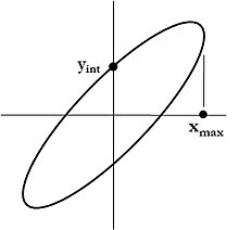
The area enclosed by a tilted ellipse is ${displaystyle pi ;y_{text{int}},x_{text{max}}}$ .

So far we have dealt with erect ellipses, whose major and minor axes are parallel to the and axes. However, some applications require tilted ellipses. In charged-particle beam optics, for instance, the enclosed area of an erect or tilted ellipse is an important property of the beam, its emittance. In this case a simple formula still applies, namely

${displaystyle A_{text{ellipse}}=pi ;y_{text{int}},x_{text{max}}=pi ;x_{text{int}},y_{text{max}}}$

(3)

where ${displaystyle y_{text{int}}}$ , ${displaystyle x_{text{int}}}$ are intercepts and ${displaystyle x_{text{max}}}$ , ${displaystyle y_{text{max}}}$ are maximum values. It follows directly from Apollonios’s theorem.

Circumference[edit]

Ellipses with same circumference

The circumference of an ellipse is:

${displaystyle C,=,4aint _{0}^{pi /2}{sqrt {1-e^{2}sin ^{2}theta }} dtheta ,=,4a,E(e)}$

where again is the length of the semi-major axis, ${textstyle e={sqrt {1-b^{2}/a^{2}}}}$ is the eccentricity, and the function is the complete elliptic integral of the second kind,

${displaystyle E(e),=,int _{0}^{pi /2}{sqrt {1-e^{2}sin ^{2}theta }} dtheta }$

which is in general not an elementary function.

The circumference of the ellipse may be evaluated in terms of E(e) using Gauss’s arithmetic-geometric mean;^[16] this is a quadratically converging iterative method (see here for details).

The exact infinite series is:

${displaystyle {begin{aligned}C&=2pi aleft[{1-left({frac {1}{2}}right)^{2}e^{2}-left({frac {1cdot 3}{2cdot 4}}right)^{2}{frac {e^{4}}{3}}-left({frac {1cdot 3cdot 5}{2cdot 4cdot 6}}right)^{2}{frac {e^{6}}{5}}-cdots }right]\&=2pi aleft[1-sum _{n=1}^{infty }left({frac {(2n-1)!!}{(2n)!!}}right)^{2}{frac {e^{2n}}{2n-1}}right]\&=-2pi asum _{n=0}^{infty }left({frac {(2n-1)!!}{(2n)!!}}right)^{2}{frac {e^{2n}}{2n-1}},end{aligned}}}$

where n!! is the double factorial (extended to negative odd integers by the recurrence relation , for ). This series converges, but by expanding in terms of ${displaystyle h=(a-b)^{2}/(a+b)^{2},}$ James Ivory^[17] and Bessel^[18] derived an expression that converges much more rapidly:

${displaystyle {begin{aligned}C&=pi (a+b)sum _{n=0}^{infty }left({frac {(2n-3)!!}{2^{n}n!}}right)^{2}h^{n}\&=pi (a+b)left[1+{frac {h}{4}}+sum _{n=2}^{infty }left({frac {(2n-3)!!}{2^{n}n!}}right)^{2}h^{n}right]\&=pi (a+b)left[1+sum _{n=1}^{infty }left({frac {(2n-1)!!}{2^{n}n!}}right)^{2}{frac {h^{n}}{(2n-1)^{2}}}right].end{aligned}}}$

Srinivasa Ramanujan gave two close approximations for the circumference in §16 of «Modular Equations and Approximations to «;^[19] they are

${displaystyle Capprox pi {biggl [}3(a+b)-{sqrt {(3a+b)(a+3b)}}{biggr ]}=pi {biggl [}3(a+b)-{sqrt {10ab+3left(a^{2}+b^{2}right)}}{biggr ]}}$

and

${displaystyle Capprox pi left(a+bright)left(1+{frac {3h}{10+{sqrt {4-3h}}}}right),}$

where takes on the same meaning as above. The errors in these approximations, which were obtained empirically, are of order $h^{3}$ and ${displaystyle h^{5},}$ respectively.

Arc length[edit]

More generally, the arc length of a portion of the circumference, as a function of the angle subtended (or x coordinates of any two points on the upper half of the ellipse), is given by an incomplete elliptic integral. The upper half of an ellipse is parameterized by

${displaystyle y=b {sqrt {1-{frac {x^{2}}{a^{2}}} }}~.}$

Then the arc length from ${displaystyle x_{1} }$ to ${displaystyle x_{2} }$ is:

${displaystyle s=-bint _{arccos {frac {x_{1}}{a}}}^{arccos {frac {x_{2}}{a}}}{sqrt { 1+left({tfrac {a^{2}}{b^{2}}}-1right) sin ^{2}z~}};mathrm {d} z~.}$

This is equivalent to

${displaystyle s=b left[;Eleft(z;{Biggl |};1-{frac {a^{2}}{b^{2}}}right);right]_{z = arccos {frac {x_{2}}{a}}}^{arccos {frac {x_{1}}{a}}}}$

where is the incomplete elliptic integral of the second kind with parameter ${displaystyle m=k^{2}.}$

Some lower and upper bounds on the circumference of the canonical ellipse ${displaystyle x^{2}/a^{2}+y^{2}/b^{2}=1 }$ with are^[20]

${displaystyle {begin{aligned}2pi b&leq Cleq 2pi a ,\pi (a+b)&leq Cleq 4(a+b) ,\4{sqrt {a^{2}+b^{2} }}&leq Cleq {sqrt {2 }}pi {sqrt {a^{2}+b^{2} }}~.end{aligned}}}$

Here the upper bound is the circumference of a circumscribed concentric circle passing through the endpoints of the ellipse’s major axis, and the lower bound $4{sqrt {a^{2}+b^{2}}}$ is the perimeter of an inscribed rhombus with vertices at the endpoints of the major and the minor axes.

Curvature[edit]

The curvature is given by ${displaystyle kappa ={frac {1}{a^{2}b^{2}}}left({frac {x^{2}}{a^{4}}}+{frac {y^{2}}{b^{4}}}right)^{-{frac {3}{2}}} ,}$
radius of curvature at point (x,y) :

${displaystyle rho =a^{2}b^{2}left({frac {x^{2}}{a^{4}}}+{frac {y^{2}}{b^{4}}}right)^{frac {3}{2}}={frac {1}{a^{4}b^{4}}}{sqrt {left(a^{4}y^{2}+b^{4}x^{2}right)^{3}}} .}$

Radius of curvature at the two vertices and the centers of curvature:

${displaystyle rho _{0}={frac {b^{2}}{a}}=p ,qquad left(pm {frac {c^{2}}{a}},{bigg |},0right) .}$

Radius of curvature at the two co-vertices and the centers of curvature:

${displaystyle rho _{1}={frac {a^{2}}{b}} ,qquad left(0,{bigg |},pm {frac {c^{2}}{b}}right) .}$

In triangle geometry[edit]

Ellipses appear in triangle geometry as

Steiner ellipse: ellipse through the vertices of the triangle with center at the centroid,
inellipses: ellipses which touch the sides of a triangle. Special cases are the Steiner inellipse and the Mandart inellipse.

As plane sections of quadrics[edit]

Ellipses appear as plane sections of the following quadrics:

Ellipsoid
Elliptic cone
Elliptic cylinder
Hyperboloid of one sheet
Hyperboloid of two sheets

Ellipsoid
Elliptic cone
Elliptic cylinder
Hyperboloid of one sheet
Hyperboloid of two sheets

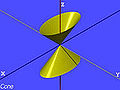
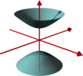
Applications[edit]

Physics[edit]

Elliptical reflectors and acoustics[edit]

Wave pattern of a little droplet dropped into mercury in one focus of the ellipse

If the water’s surface is disturbed at one focus of an elliptical water tank, the circular waves of that disturbance, after reflecting off the walls, converge simultaneously to a single point: the second focus. This is a consequence of the total travel length being the same along any wall-bouncing path between the two foci.

Similarly, if a light source is placed at one focus of an elliptic mirror, all light rays on the plane of the ellipse are reflected to the second focus. Since no other smooth curve has such a property, it can be used as an alternative definition of an ellipse. (In the special case of a circle with a source at its center all light would be reflected back to the center.) If the ellipse is rotated along its major axis to produce an ellipsoidal mirror (specifically, a prolate spheroid), this property holds for all rays out of the source. Alternatively, a cylindrical mirror with elliptical cross-section can be used to focus light from a linear fluorescent lamp along a line of the paper; such mirrors are used in some document scanners.

Sound waves are reflected in a similar way, so in a large elliptical room a person standing at one focus can hear a person standing at the other focus remarkably well. The effect is even more evident under a vaulted roof shaped as a section of a prolate spheroid. Such a room is called a whisper chamber. The same effect can be demonstrated with two reflectors shaped like the end caps of such a spheroid, placed facing each other at the proper distance. Examples are the National Statuary Hall at the United States Capitol (where John Quincy Adams is said to have used this property for eavesdropping on political matters); the Mormon Tabernacle at Temple Square in Salt Lake City, Utah; at an exhibit on sound at the Museum of Science and Industry in Chicago; in front of the University of Illinois at Urbana–Champaign Foellinger Auditorium; and also at a side chamber of the Palace of Charles V, in the Alhambra.

Planetary orbits[edit]

In the 17th century, Johannes Kepler discovered that the orbits along which the planets travel around the Sun are ellipses with the Sun [approximately] at one focus, in his first law of planetary motion. Later, Isaac Newton explained this as a corollary of his law of universal gravitation.

More generally, in the gravitational two-body problem, if the two bodies are bound to each other (that is, the total energy is negative), their orbits are similar ellipses with the common barycenter being one of the foci of each ellipse. The other focus of either ellipse has no known physical significance. The orbit of either body in the reference frame of the other is also an ellipse, with the other body at the same focus.

Keplerian elliptical orbits are the result of any radially directed attraction force whose strength is inversely proportional to the square of the distance. Thus, in principle, the motion of two oppositely charged particles in empty space would also be an ellipse. (However, this conclusion ignores losses due to electromagnetic radiation and quantum effects, which become significant when the particles are moving at high speed.)

For elliptical orbits, useful relations involving the eccentricity are:

${displaystyle {begin{aligned}e&={frac {r_{a}-r_{p}}{r_{a}+r_{p}}}={frac {r_{a}-r_{p}}{2a}}\r_{a}&=(1+e)a\r_{p}&=(1-e)aend{aligned}}}$

where

Also, in terms of $r_{a}$ and $r_{p}$ , the semi-major axis is their arithmetic mean, the semi-minor axis is their geometric mean, and the semi-latus rectum ell is their harmonic mean. In other words,

${displaystyle {begin{aligned}a&={frac {r_{a}+r_{p}}{2}}\[2pt]b&={sqrt {r_{a}r_{p}}}\[2pt]ell &={frac {2}{{frac {1}{r_{a}}}+{frac {1}{r_{p}}}}}={frac {2r_{a}r_{p}}{r_{a}+r_{p}}}end{aligned}}}$

Harmonic oscillators[edit]

The general solution for a harmonic oscillator in two or more dimensions is also an ellipse. Such is the case, for instance, of a long pendulum that is free to move in two dimensions; of a mass attached to a fixed point by a perfectly elastic spring; or of any object that moves under influence of an attractive force that is directly proportional to its distance from a fixed attractor. Unlike Keplerian orbits, however, these «harmonic orbits» have the center of attraction at the geometric center of the ellipse, and have fairly simple equations of motion.

Phase visualization[edit]

In electronics, the relative phase of two sinusoidal signals can be compared by feeding them to the vertical and horizontal inputs of an oscilloscope. If the Lissajous figure display is an ellipse, rather than a straight line, the two signals are out of phase.

Elliptical gears[edit]

Two non-circular gears with the same elliptical outline, each pivoting around one focus and positioned at the proper angle, turn smoothly while maintaining contact at all times. Alternatively, they can be connected by a link chain or timing belt, or in the case of a bicycle the main chainring may be elliptical, or an ovoid similar to an ellipse in form. Such elliptical gears may be used in mechanical equipment to produce variable angular speed or torque from a constant rotation of the driving axle, or in the case of a bicycle to allow a varying crank rotation speed with inversely varying mechanical advantage.

Elliptical bicycle gears make it easier for the chain to slide off the cog when changing gears.^[21]

An example gear application would be a device that winds thread onto a conical bobbin on a spinning machine. The bobbin would need to wind faster when the thread is near the apex than when it is near the base.^[22]

Optics[edit]

In a material that is optically anisotropic (birefringent), the refractive index depends on the direction of the light. The dependency can be described by an index ellipsoid. (If the material is optically isotropic, this ellipsoid is a sphere.)
In lamp-pumped solid-state lasers, elliptical cylinder-shaped reflectors have been used to direct light from the pump lamp (coaxial with one ellipse focal axis) to the active medium rod (coaxial with the second focal axis).^[23]
In laser-plasma produced EUV light sources used in microchip lithography, EUV light is generated by plasma positioned in the primary focus of an ellipsoid mirror and is collected in the secondary focus at the input of the lithography machine.^[24]

Statistics and finance[edit]

In statistics, a bivariate random vector (X,Y) is jointly elliptically distributed if its iso-density contours—loci of equal values of the density function—are ellipses. The concept extends to an arbitrary number of elements of the random vector, in which case in general the iso-density contours are ellipsoids. A special case is the multivariate normal distribution. The elliptical distributions are important in finance because if rates of return on assets are jointly elliptically distributed then all portfolios can be characterized completely by their mean and variance—that is, any two portfolios with identical mean and variance of portfolio return have identical distributions of portfolio return.^[25]^[26]

Computer graphics[edit]

Drawing an ellipse as a graphics primitive is common in standard display libraries, such as the MacIntosh QuickDraw API, and Direct2D on Windows. Jack Bresenham at IBM is most famous for the invention of 2D drawing primitives, including line and circle drawing, using only fast integer operations such as addition and branch on carry bit. M. L. V. Pitteway extended Bresenham’s algorithm for lines to conics in 1967.^[27] Another efficient generalization to draw ellipses was invented in 1984 by Jerry Van Aken.^[28]

In 1970 Danny Cohen presented at the «Computer Graphics 1970» conference in England a linear algorithm for drawing ellipses and circles. In 1971, L. B. Smith published similar algorithms for all conic sections and proved them to have good properties.^[29] These algorithms need only a few multiplications and additions to calculate each vector.

It is beneficial to use a parametric formulation in computer graphics because the density of points is greatest where there is the most curvature. Thus, the change in slope between each successive point is small, reducing the apparent «jaggedness» of the approximation.

Drawing with Bézier paths

Composite Bézier curves may also be used to draw an ellipse to sufficient accuracy, since any ellipse may be construed as an affine transformation of a circle. The spline methods used to draw a circle may be used to draw an ellipse, since the constituent Bézier curves behave appropriately under such transformations.

Optimization theory[edit]

It is sometimes useful to find the minimum bounding ellipse on a set of points. The ellipsoid method is quite useful for solving this problem.

Notes[edit]

^ Apostol, Tom M.; Mnatsakanian, Mamikon A. (2012), New Horizons in Geometry, The Dolciani Mathematical Expositions #47, The Mathematical Association of America, p. 251, ISBN 978-0-88385-354-2
^ The German term for this circle is Leitkreis which can be translated as «Director circle», but that term has a different meaning in the English literature (see Director circle).
^ «Ellipse — from Wolfram MathWorld». Mathworld.wolfram.com. 2020-09-10. Retrieved 2020-09-10.
^ Protter & Morrey (1970, pp. 304, APP-28)
^ Larson, Ron; Hostetler, Robert P.; Falvo, David C. (2006). «Chapter 10». Precalculus with Limits. Cengage Learning. p. 767. ISBN 978-0-618-66089-6.
^ Young, Cynthia Y. (2010). «Chapter 9». Precalculus. John Wiley and Sons. p. 831. ISBN 978-0-471-75684-2.
^ ^a ^b Lawrence, J. Dennis, A Catalog of Special Plane Curves, Dover Publ., 1972.
^ K. Strubecker: Vorlesungen über Darstellende Geometrie, GÖTTINGEN,
VANDENHOECK & RUPRECHT, 1967, p. 26
^ Bronstein&Semendjajew: Taschenbuch der Mathematik, Verlag Harri Deutsch, 1979, ISBN 3871444928, p. 274.
^ Encyclopedia of Mathematics, Springer, URL: http://encyclopediaofmath.org/index.php?title=Apollonius_theorem&oldid=17516 .
^ K. Strubecker: Vorlesungen über Darstellende Geometrie. Vandenhoeck & Ruprecht, Göttingen 1967, S. 26.
^ J. van Mannen: Seventeenth century instruments for drawing conic sections. In: The Mathematical Gazette. Vol. 76, 1992, p. 222–230.
^ E. Hartmann: Lecture Note ‘Planar Circle Geometries’, an Introduction to Möbius-, Laguerre- and Minkowski Planes, p. 55
^ W. Benz, Vorlesungen über Geomerie der Algebren, Springer (1973)
^ Archimedes. (1897). The works of Archimedes. Heath, Thomas Little, Sir, 1861-1940. Mineola, N.Y.: Dover Publications. p. 115. ISBN 0-486-42084-1. OCLC 48876646.
^ Carlson, B. C. (2010), «Elliptic Integrals», in Olver, Frank W. J.; Lozier, Daniel M.; Boisvert, Ronald F.; Clark, Charles W. (eds.), NIST Handbook of Mathematical Functions, Cambridge University Press, ISBN 978-0-521-19225-5, MR 2723248
^ Ivory, J. (1798). «A new series for the rectification of the ellipsis». Transactions of the Royal Society of Edinburgh. 4 (2): 177–190. doi:10.1017/s0080456800030817. S2CID 251572677.
^ Bessel, F. W. (2010). «The calculation of longitude and latitude from geodesic measurements (1825)». Astron. Nachr. 331 (8): 852–861. arXiv:0908.1824. Bibcode:2010AN….331..852K. doi:10.1002/asna.201011352. S2CID 118760590. Englisch translation of Bessel, F. W. (1825). «Über die Berechnung der geographischen Längen und Breiten aus geodätischen Vermesssungen». Astron. Nachr. 4 (16): 241–254. arXiv:0908.1823. Bibcode:1825AN……4..241B. doi:10.1002/asna.18260041601. S2CID 118630614.
^ Ramanujan, Srinivasa (1914). «Modular Equations and Approximations to π». Quart. J. Pure App. Math. 45: 350–372. ISBN 9780821820766.
^ Jameson, G.J.O. (2014). «Inequalities for the perimeter of an ellipse». Mathematical Gazette. 98 (542): 227–234. doi:10.1017/S002555720000125X. S2CID 125063457.
^ David Drew.
«Elliptical Gears».
[1]
^ Grant, George B. (1906). A treatise on gear wheels. Philadelphia Gear Works. p. 72.
^ Encyclopedia of Laser Physics and Technology — lamp-pumped lasers, arc lamps, flash lamps, high-power, Nd:YAG laser
^ «Cymer — EUV Plasma Chamber Detail Category Home Page». Archived from the original on 2013-05-17. Retrieved 2013-06-20.
^ Chamberlain, G. (February 1983). «A characterization of the distributions that imply mean—Variance utility functions». Journal of Economic Theory. 29 (1): 185–201. doi:10.1016/0022-0531(83)90129-1.
^ Owen, J.; Rabinovitch, R. (June 1983). «On the class of elliptical distributions and their applications to the theory of portfolio choice». Journal of Finance. 38 (3): 745–752. doi:10.1111/j.1540-6261.1983.tb02499.x. JSTOR 2328079.
^ Pitteway, M.L.V. (1967). «Algorithm for drawing ellipses or hyperbolae with a digital plotter». The Computer Journal. 10 (3): 282–9. doi:10.1093/comjnl/10.3.282.
^ Van Aken, J.R. (September 1984). «An Efficient Ellipse-Drawing Algorithm». IEEE Computer Graphics and Applications. 4 (9): 24–35. doi:10.1109/MCG.1984.275994. S2CID 18995215.
^ Smith, L.B. (1971). «Drawing ellipses, hyperbolae or parabolae with a fixed number of points». The Computer Journal. 14 (1): 81–86. doi:10.1093/comjnl/14.1.81.

References[edit]

Besant, W.H. (1907). «Chapter III. The Ellipse». Conic Sections. London: George Bell and Sons. p. 50.
Coxeter, H.S.M. (1969). Introduction to Geometry (2nd ed.). New York: Wiley. pp. 115–9.
Meserve, Bruce E. (1983) [1959], Fundamental Concepts of Geometry, Dover Publications, ISBN 978-0-486-63415-9
Miller, Charles D.; Lial, Margaret L.; Schneider, David I. (1990). Fundamentals of College Algebra (3rd ed.). Scott Foresman/Little. p. 381. ISBN 978-0-673-38638-0.
Protter, Murray H.; Morrey, Charles B. Jr. (1970), College Calculus with Analytic Geometry (2nd ed.), Reading: Addison-Wesley, LCCN 76087042

External links[edit]

Источник

Определение и элементы эллипса

По форме график эллипса представляет замкнутую овальную кривую:

Точки эллипса, являющиеся концами осей, называются вершинами.

Расстояния от точки на линии до фокусов получили название фокальных радиусов.

Расстояние между фокусами есть фокальное расстояние.

Основные свойства эллипса

Их несколько:

имеются две оси и один центр симметрии;
при равенстве полуосей линия превращается в окружность;
все точки фигуры лежат внутри прямоугольника со сторонами, равными большой и малой осям эллипса, проходящими через вершины параллельно осям.

Уравнение эллипса

Пусть линия расположена так, чтобы центр симметрии совпадал с началом координат, а оси – с осями координат.

Для составления уравнения достаточно воспользоваться определением, введя обозначение:

а – большая полуось (в наиболее простом виде её располагают вдоль оси Оx) (большая ось, соответственно, равна 2a);
c – половина фокального расстояния;
M(x;y) – произвольная точка линии.

В этом случае фокусы находятся в точках F₁(-c;0); F₂(c;0)

Согласно определению,

MF₁ + MF₂ = 2a,

поэтому

100

101

После ввода ещё одного обозначения

b² = a² — c²

получается наиболее простой вид уравнения:

a²b² — a²y² — x²b² = 0,

a²b² = a²y² + x²b²,

Параметр b численно равен полуоси, расположенной вдоль Oy (a > b).

В случае (b < a) уравнение не изменится, однако, будет выполняться условие

Такое уравнение называется каноническим, то есть наиболее простым.

Каждое слагаемое в левой части не превосходит единицу.

При возрастании значения lxl уменьшается lyl и наоборот.

В случае (a > b) формула эксцентриситета (ε) принимает вид:

если b > a, то

Чем меньше эксцентриситет, тем более сжатым будет эллипс.

Площадь эллипса

Площадь фигуры (овала), ограниченной эллипсом, можно вычислить по формуле:

a – большая полуось, b – малая.

Площадь сегмента эллипса

Часть эллипса, отсекаемая прямой, называется его сегментом.

, где

(x_o;y₀) – крайняя точка сегмента.

Длина дуги эллипса

Длина дуги находится с помощью определённого интеграла по соответствующей формуле при введении параметра:

Радиус круга, вписанного в эллипс

r = b.

Радиус круга, описанного вокруг эллипса

R = a.

Как построить эллипс

Построение линии удобно выполнять в декартовых координатах в каноническом виде.

Отмечаются вершины:

Строится прямоугольник. Для этого проводятся прямые:

Сглаживая углы, проводится линия по сторонам прямоугольника.

Полученная фигура есть эллипс. По координатам отмечается каждый фокус.

При вращении вокруг любой из осей координат образуется поверхность, которая называется эллипсоид.

Источник

Калькулятор

Длина дуги, как сумма хорд

Длина дуги, как интеграл

Длина дуги через эксцентриситет

Длина дуги через эксцентриситет с подготовкой

Длина дуги и хорошо забытые хорды

Практика

Небольшая инструкция

Скачать

Определение эллипсa

Элементы эллипсa

Основные свойства эллипсa

Уравнение эллипсa

Каноническое уравнение эллипсa:

Параметрическое уравнение эллипсa:

Радиус круга вписанного в эллипс

Радиус круга описанного вокруг эллипсa

Площадь эллипсa

Площадь сегмента эллипсa

Периметр эллипсa

Длина дуги эллипсa

Формулы определения длины дуги эллипсa:

Эллипс — свойства, уравнение и построение фигуры

Определение и элементы эллипса

Основные свойства эллипса

Уравнение эллипса

Площадь эллипса

Площадь сегмента эллипса

Длина дуги эллипса

Радиус круга, вписанного в эллипс

Радиус круга, описанного вокруг эллипса

Как построить эллипс

Чертежик

Метки

Построение овала

Урок 3. Окружность в перспективе. Как нарисовать кружку и вазу

Принципы рисования эллипсов:

Рисуем эллипсы

Рисуем кружку

Рисуем вазу

Проверьте свои знания

Definition as locus of points[edit]

In Cartesian coordinates[edit]

Standard equation[edit]

Parameters[edit]

Principal axes[edit]

Linear eccentricity[edit]

Eccentricity[edit]

Semi-latus rectum[edit]

Tangent[edit]

Shifted ellipse[edit]

General ellipse[edit]

Parametric representation[edit]

Standard parametric representation[edit]

Rational representation[edit]

Tangent slope as parameter[edit]

General ellipse[edit]

Polar forms[edit]

Polar form relative to center[edit]

Polar form relative to focus[edit]

Eccentricity and the directrix property[edit]

Focus-to-focus reflection property[edit]

Conjugate diameters[edit]

Definition of conjugate diameters[edit]

Theorem of Apollonios on conjugate diameters[edit]

Orthogonal tangents[edit]

Drawing ellipses[edit]

de La Hire’s point construction[edit]

Pins-and-string method[edit]

Paper strip methods[edit]

Approximation by osculating circles[edit]

Steiner generation[edit]

As hypotrochoid[edit]

Inscribed angles and three-point form[edit]

Circles[edit]

Inscribed angle theorem for circles[edit]

Three-point form of circle equation[edit]

Ellipses[edit]

Inscribed angle theorem for ellipses[edit]

Three-point form of ellipse equation[edit]