4.2. Эластичность спроса и предложения
4.2.1. Общее понятие эластичности. Эластичность спроса
Реакция покупателей и продавцов на изменяющуюся рыночную конъюнктуру, в частности, на изменение цены может быть различной по своей интенсивности. Так, очевидно, что по-разному отреагируют покупатели при уменьшении цен на автомобили и французские духи, с одной стороны, и хлеб и молоко — с другой: в одном случае объем продаж может существенно возрасти, в другом — изменится мало.
Общее понятие эластичности
Для характеристики степени влияния изменения цены на поведение покупателей и продавцов в экономике используется понятие эластичность, которую можно определить как степень реакции одной величины на изменение другой.
Данное понятие весьма важно с практической точки зрения. Так, проведение разумной ценовой политики фирмой немыслимо без понимания того, как понижение стоимости телевизоров или стиральных машин может сказаться на объемах их продаж, а значит, и на выручке. Подсчитывать (измерять), как изменяется объем продаж или покупок того или иного товара в ответ на изменение цены, можно по-разному, например, в штуках, в тоннах, в тех или иных денежных единицах. Но все эти подходы требуют дополнительной информации и сами по себе мало о чем говорят.
Так, фраза: «Увеличение цены колбасы на 5 руб. вызвало сокращение ее продаж на 12 т», без дополнительных разъяснений почти бессмысленна. Велико ли было изменение цен? Если дело происходило в 1997 г. и она стоила 25000 руб., то, конечно, невелико. А если в начале 1998 г. при исходной цене 25 руб., то его вполне можно признать значительным. Столь же неясно, насколько катастрофично снижение продаж. Одно дело, если первоначальный уровень составлял 50 т и совсем другое, если — 500 т.
Коэффициент эластичности
Оценка эластичности в процентном исчислении позволяет избежать подобной путаницы и построить единый показатель для всех случаев. Такой показатель называют коэффициентом эластичности. Его можно определить как отношение процентного изменения одной величины к процентному изменению другой.
Эластичность спроса по цене
Зависимость изменения спроса на товар от изменения его цены называется эластичностью спроса по цене, или ценовой эластичностью. Принято различать три варианта ценовой эластичности спроса.
- эластичный спрос, когда при незначительных понижениях цены объем продаж значительно возрастает.
- единичная эластичность спроса, когда изменение цены, выраженное в процентах, равно проценту изменения объема продаж.
- неэластичный спрос, если вслед за изменением цены не происходит существенного изменения продаж.
Величина эластичности спроса
Эластичность можно измерить с помощью уже упомянутого коэффициента эластичности. Представим его в виде формулы
Приведенная формула позволяет количественно определить все три варианта ценовой эластичности спроса. Так, в случае эластичного спроса, когда прирост количества больше уменьшения цены, величина коэффициента превышает единицу ( ); при неэластичном спросе, напротив,
  ; а в случае спроса единичной эластичности, когда процентное изменение цены строго равно изменению количества, устанавливается равенство
  (от которого, собственно, и пошло название единичная эластичность).
Рис.
4.14.
Графическая интерпретация спроса с различной эластичностью
Эластичным спрос по цене бывает, как правило, для предметов роскоши — драгоценностей, мехов, черной икры и т.п., и для достаточно дорогих предметов потребления, как автомобили, телевизоры, стиральные машины, аудио- и видеотехника, персональные компьютеры и др. Неэластичен спрос на товары первой необходимости с относительно низкими ценами — на хлеб, картофель, одежду, обувь, белье, расходы на общественный транспорт и пр.
Давая графическую интерпретацию эластичности (
рис.
4.14), обратим внимание на то, что, чем больше коэффициент эластичности, тем в принципе более пологая кривая спроса. А чем меньше он, тем более круто (опять-таки, в принципе — уточнение см. ниже) падает кривая.
Кроме рассмотренных трех случаев эластичности спроса по цене, можно указать еще два — абсолютно эластичный спрос и абсолютно неэластичный спрос. На
рис.
4.15 даны графики спроса для этих двух случаев.
Рис.
4.15.
Экстремальные случаи эластичности спроса: а) абсолютно эластичный; б) абсолютно неэластичный
В случае абсолютно эластичного спроса — это горизонтальная кривая спроса (
рис.
4.15 а) — потребители платят одну и ту же цену за товар, невзирая на величину спроса ( ). В случае абсолютно неэластичного спроса они покупают одно и то же количество товара при любых уровнях цен. То есть изменение цены не вызывает никакого изменения спроса (Е = 0), а кривая вырождается в вертикальную прямую (
рис.
4.15 б).
В качестве примера спроса, приближающегося к абсолютно неэластичному, можно указать на ситуацию с некоторыми медикаментами. Например, спрос на инсулин для больных сахарным диабетом (без него человек может умереть, а при правильном приеме нормально доживает до старости). Абсолютно эластичный спрос характерен для ситуации совершенной конкуренции (см.
«Издержки»
), когда производители не могут влиять на цену, а покупатели готовы приобретать любое количество товаров по данной цене.
Особенно важны экстремальные случаи эластичности как полезные абстракции, позволяющие понять суть многих экономических процессов.
Особенности графической интерпретации эластичности
Хотя мы и проиллюстрировали различные виды эластичности кривыми спроса с разными углами наклона, однако не следует напрямую отождествлять наклон кривой спроса и эластичность. Разумеется, обе величины связаны между собой. Ясно, например, что очень пологие кривые спроса будут весьма эластичны: малое изменение цены на них порождает большое изменение объема спроса. И все же это не одно и то же. Наклон кривой на обычном графике отражает абсолютные изменения цены и количества, а эластичность — процентные изменения.
На
рис.
4.16 а показана кривая спроса, имеющая на всем протяжении одинаковый наклон (именно поэтому эта кривая и выглядит, как прямая). Убедимся, что она имеет различную эластичность в различных точках. В верхней части кривой (на графике — точки 1 и 2) спрос эластичен, поскольку при малом процентном изменении цены (отношение  ) велико процентное изменение количества (отношение
  ).
).

Рис.
4.16.
Эластичность на различных участках прямой линии
В нижней части кривой ситуация меняется на противоположную. Чтобы сделать это наглядным, мы специально повторили ту же самую кривую еще раз на графике 4.16 б и выделили точки 3 и 4 в ее нижней части. Сразу бросается в глаза, что процентное изменение цены (отношение  ) здесь велико — она упала чуть ли не вдвое. Напротив, процентное изменение количества (отношение
  ) мало — оно выросло лишь на незначительную долю исходной величины.
В силу описанных обстоятельств изображение более или менее эластичного спроса в виде кривых разного наклона следует рассматривать лишь как приблизительную иллюстрацию. Для простоты мы будем пользоваться такими графиками и в дальнейшем. Чтобы придать графическим изображениям математическую точность их, однако, следует строить в так называемых двойных логарифмических шкалах, где каждое новое деление осей координат изображается в 10 раз более сжатом масштабе. Не заостряя на этом специального внимания, мы уже использовали такие шкалы на
рис.
4.14.
Только в двойных логарифмических шкалах угол наклона кривой точно соответствует величине ее эластичности. Исключение из этого правила составляют абсолютно эластичные и абсолютно неэластичные кривые спроса, каждая точка которых имеет и один и тот же наклон и одну и ту же эластичность даже на обычных графиках.
Эластичность спроса и объем выручки
Изменение объема продаж, к которому мы апеллировали, давая определение эластичности спроса по цене, влияет на объем выручки и финансовое положение продавца. Ведь зная размеры спроса, можно легко вычислить объем выручки — это произведение  или площадь прямоугольника, одна сторона которого равна цене товара, а вторая — количеству товара, проданного по этой цене. Проанализируем ситуацию с объемом выручки при различных вариантах эластичности графически. На
рис.
4.17 показано, как изменяется общая выручка при одинаковом изменении цены для товаров с различной эластичностью спроса:
- при эластичном спросе снижение цены вызывает такое увеличение объема продаж, которое ведет к увеличению общей выручки (площадь прямоугольника, соответствующего низкой цене, явно больше площади прямоугольника, соответствующего высокой цене).
- при спросе единичной эластичности прирост объема продаж при снижении цены таков, что общая выручка остается неизменной (обе площади равны).
- при неэластичном спросе снижение цены ведет к столь малому увеличению продаж, что объем общей выручки уменьшается (площадь прямоугольника, соответствующего низкой цене, меньше площади прямоугольника, соответствующего высокой цене).
Рис.
4.17.
Рис. 4.17. Изменение выручки продавца при различной эластичности спроса: а) эластичный спрос; б) спрос единичной эластичности; в) неэластичный спрос
Факторы эластичности спроса
Эластичность спроса по цене зависит от ряда факторов, к которым относятся следующие:
- незаменимость. Если у товара есть заменители (товары-субституты), то спрос будет более эластичным, противоположным образом влияет отсутствие таковых;
- значимость товара для потребителя. Как правило, неэластичным является спрос на товары первой необходимости, а более эластичным — на все другие группы товаров;
- удельный вес в доходах и расходах. Товары, на которые тратится значительная доля средств, эластичны, а занимающие незначительную долю бюджета — неэластичны.
- временные рамки. Эластичность спроса увеличивается в долгосрочном плане и становится менее эластичной на коротких промежутках времени.
Эластичность спроса по доходу
Кроме эластичности спроса по цене, важный экономический смысл имеет также эластичность спроса по доходу, которую можно определить как отношение процентного изменения объема спроса на товар к процентному изменению дохода (I):

Поскольку потребитель по-разному меняет спрос на различные товары при изменении дохода, то и показатель может иметь различные положительные и отрицательные значения. Так, если потребитель увеличивает объем закупок при возрастании дохода, то эластичность по доходу положительна ( ). В этом случае речь идет, скорее всего, о стандартном нормальном товаре, допустим, дополнительных парах обуви, которую потребитель может позволить себе купить при возрастании дохода. Если при этом рост спроса опережает рост дохода (
 ), то говорят о высокой эластичности спроса по доходу. Так бывает, в частности, со спросом на товары длительного пользования, например, автомобили или персональные компьютеры, для приобретения которых люди берут кредит или тратят сбережения.
Но возможна и противоположная ситуация, когда значение  отрицательно (
 ). Это могут быть аномальные или низкокачественные товары (дешевые сорта колбасы, сигарет, маргарин и т.п.), т.е. те товары, которые потребители при растущем доходе покупают, как правило, меньше, заменяя их более качественными товарами (см. 4.1.1).
Перекрестная эластичность
Как мы уже отмечали, реакция потребителей на изменение цены зависит от цен на другие товары. Зависимость эластичности спроса на одно благо относительно изменения цен на другие блага называется перекрестной эластичностью, которая измеряется как отношение процентного изменения спроса на товар А к процентному изменению цены на товар В:
Перекрестная эластичность показывает наличие связи в потреблении между рассматриваемыми товарами. Если  , т.е. с повышением цены на товар В растет спрос на товар А, то речь идет о взаимозаменяемых товарах (товарах-субститутах). Например, рост цен на американские куриные окорочка заставляет покупателей переходить на относительно дешевую российскую рыбу, а подорожавший рис заменять более дешевым картофелем.
Если  , т.е. повышение цен на товар ведет к уменьшению спроса на товар А, то мы имеем дело с взаимодополняющими товарами: так, рост цен на фотопленку уменьшает спрос на фотоаппараты.
Наконец, товары могут быть индифферентны друг к другу ( ), т.е. изменение цен на один из них ничего не меняет в количественном спросе на другой, например, растущие цены на автомобили не влияют на количество покупаемой соли.
A good’s price elasticity of demand ( , PED) is a measure of how sensitive the quantity demanded is to its price. When the price rises, quantity demanded falls for almost any good, but it falls more for some than for others. The price elasticity gives the percentage change in quantity demanded when there is a one percent increase in price, holding everything else constant. If the elasticity is −2, that means a one percent price rise leads to a two percent decline in quantity demanded. Other elasticities measure how the quantity demanded changes with other variables (e.g. the income elasticity of demand for consumer income changes).[1]
Price elasticities are negative except in special cases. If a good is said to have an elasticity of 2, it almost always means that the good has an elasticity of −2 according to the formal definition. The phrase «more elastic» means that a good’s elasticity has greater magnitude, ignoring the sign. Veblen and Giffen goods are two classes of goods which have positive elasticity, rare exceptions to the law of demand. Demand for a good is said to be inelastic when the elasticity is less than one in absolute value: that is, changes in price have a relatively small effect on the quantity demanded. Demand for a good is said to be elastic when the elasticity is greater than one. A good with an elasticity of −2 has elastic demand because quantity falls twice as much as the price increase; an elasticity of −0.5 has inelastic demand because the quantity response is half the price increase.[2]
At an elasticity of 0 consumption would not change at all, in spite of any price increases.
Revenue is maximised when price is set so that the elasticity is exactly one. The good’s elasticity can be used to predict the incidence (or «burden») of a tax on that good. Various research methods are used to determine price elasticity, including test markets, analysis of historical sales data and conjoint analysis.
Definition[edit]
The variation in demand in response to a variation in price is called price elasticity of demand. It may also be defined as the ratio of the percentage change in quantity demanded to the percentage change in price of particular commodity.[3] The formula
for the coefficient of price elasticity of demand for a good is:[4][5][6]

where  is the initial price of the good demanded,
  is how much it changed,
  is the initial quantity of the good demanded, and
  is how much it changed. In other words, we can say that the price elasticity of demand is the percentage change in demand for a commodity due to a given percentage change in the price. If the quantity demanded falls 20 tons from an initial 200 tons after the price rises $5 from an initial price of $100, then the quantity demanded has fallen 10% and the price has risen 5%, so the elasticity is (−10%)/(+5%) = −2.
The price elasticity of demand is ordinarily negative because quantity demanded falls when price rises, as described by the «law of demand».[5] Two rare classes of goods which have elasticity greater than 0 (consumers buy more if the price is higher) are Veblen and Giffen goods.[7] Since the price elasticity of demand is negative for the vast majority of goods and services (unlike most other elasticities, which take both positive and negative values depending on the good), economists often leave off the word «negative» or the minus sign and refer to the price elasticity of demand as a positive value (i.e., in absolute value terms).[6] They will say «Yachts have an elasticity of two» meaning the elasticity is −2. This is a common source of confusion for students.
Depending on its elasticity, a good is said to have
elastic demand (> 1),
inelastic demand (< 1), or
unitary elastic demand (= 1). If demand is elastic, the quantity demanded is very sensitive to price, e.g. when a 1% rise in price generates a 10% decrease in quantity. If demand is inelastic, the good’s demand is relatively insensitive to price, with quantity changing less than price. If demand is unitary elastic, the quantity falls by exactly the percentage that the price rises. Two important special cases are perfectly elastic demand (= ∞), where even a small rise in price reduces the quantity demanded to zero; and perfectly inelastic demand (= 0), where a rise in price leaves the quantity unchanged.
The above measure of elasticity is sometimes referred to as the own-price elasticity of demand for a good, i.e., the elasticity of demand with respect to the good’s own price, in order to distinguish it from the elasticity of demand for that good with respect to the change in the price of some other good, i.e., an independent, complementary, or substitute good.[3] That two-good type of elasticity is called a cross-price elasticity of demand.[8][9] If a 1% rise in the price of gasoline causes a 0.5% fall in the quantity of cars demanded, the cross-price elasticity is 
As the size of the price change gets bigger, the elasticity definition becomes less reliable for a combination of two reasons. First, a good’s elasticity is not necessarily constant; it varies at different points along the demand curve because a 1% change in price has a quantity effect that may depend on whether the initial price is high or low.[10][11] Contrary to common misconception, the price elasticity is not constant even along a linear demand curve, but rather varies along the curve.[12] A linear demand curve’s slope is constant, to be sure, but the elasticity can change even if  is constant.[13][14] There does exist a nonlinear shape of demand curve along which the elasticity is constant:
  , where
  is a shift constant and
  is the elasticity.
Second, percentage changes are not symmetric; instead, the percentage change between any two values depends on which one is chosen as the starting value and which as the ending value. For example, suppose that when the price rises from $10 to $16, the quantity falls from 100 units to 80. This is a price increase of 60% and a quantity decline of 20%, an elasticity of  for that part of the demand curve. If the price falls from $16 to $10 and the quantity rises from 80 units to 100, however, the price decline is 37.5% and the quantity gain is 25%, an elasticity of
  for the same part of the curve. This is an example of the index number problem.[15][16]
Two refinements of the definition of elasticity are used to deal with these shortcomings of the basic elasticity formula: arc elasticity and point elasticity.
Arc elasticity[edit]
Arc elasticity was introduced very early on by Hugh Dalton. It is very similar to an ordinary elasticity problem, but it adds in the index number problem. Arc Elasticity is a second solution to the asymmetry problem of having an elasticity dependent on which of the two given points on a demand curve is chosen as the «original» point will and which as the «new» one is to compute the percentage change in P and Q relative to the average of the two prices and the average of the two quantities, rather than just the change relative to one point or the other. Loosely speaking, this gives an «average» elasticity for the section of the actual demand curve—i.e., the arc of the curve—between the two points. As a result, this measure is known as the arc elasticity, in this case with respect to the price of the good. The arc elasticity is defined mathematically as:[16][17][18]

This method for computing the price elasticity is also known as the «midpoints formula», because the average price and average quantity are the coordinates of the midpoint of the straight line between the two given points.[15][18] This formula is an application of the midpoint method. However, because this formula implicitly assumes the section of the demand curve between those points is linear, the greater the curvature of the actual demand curve is over that range, the worse this approximation of its elasticity will be.[17][19]
Point elasticity[edit]
The point elasticity of demand method is used to determine change in demand within the same demand curve, basically a very small amount of change in demand is measured through point elasticity. One way to avoid the accuracy problem described above is to minimize the difference between the starting and ending prices and quantities. This is the approach taken in the definition of point elasticity, which uses differential calculus to calculate the elasticity for an infinitesimal change in price and quantity at any given point on the demand curve:[20]

In other words, it is equal to the absolute value of the first derivative of quantity with respect to price  multiplied by the point’s price (P) divided by its quantity (Qd).[21] However, the point elasticity can be computed only if the formula for the demand function,
  , is known so its derivative with respect to price,
  , can be determined.
In terms of partial-differential calculus, point elasticity of demand can be defined as follows:[22] let  be the demand of goods
  as a function of parameters price and wealth, and let
  be the demand for good
  . The elasticity of demand for good with respect to price
  is
is

History[edit]
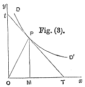
The illustration that accompanied Marshall’s original definition of elasticity, the ratio of PT to Pt
Together with the concept of an economic «elasticity» coefficient, Alfred Marshall is credited with defining «elasticity of demand» in Principles of Economics, published in 1890.[23] Alfred Marshall invented price elasticity of demand only four years after he had invented the concept of elasticity. He used Cournot’s basic creating of the demand curve to get the equation for price elasticity of demand. He described price elasticity of demand as thus: «And we may say generally:— the elasticity (or responsiveness) of demand in a market is great or small according as the amount demanded increases much or little for a given fall in price, and diminishes much or little for a given rise in price».[24] He reasons this since «the only universal law as to a person’s desire for a commodity is that it diminishes … but this diminution may be slow or rapid. If it is slow… a small fall in price will cause a comparatively large increase in his purchases. But if it is rapid, a small fall in price will cause only a very small increase in his purchases. In the former case… the elasticity of his wants, we may say, is great. In the latter case… the elasticity of his demand is small.»[25] Mathematically, the Marshallian PED was based on a point-price definition, using differential calculus to calculate elasticities.[26]
Determinants[edit]
The overriding factor in determining the elasticity is the willingness and ability of consumers after a price change to postpone immediate consumption decisions concerning the good and to search for substitutes («wait and look»).[27] A number of factors can thus affect the elasticity of demand for a good:[28]
- Availability of substitute goods
- The more and closer the substitutes available, the higher the elasticity is likely to be, as people can easily switch from one good to another if an even minor price change is made;[28][29][30] There is a strong substitution effect.[31] If no close substitutes are available, the substitution effect will be small and the demand inelastic.[31]
- Breadth of definition of a good
- The broader the definition of a good (or service), the lower the elasticity. For example, Company X’s fish and chips would tend to have a relatively high elasticity of demand if a significant number of substitutes are available, whereas food in general would have an extremely low elasticity of demand because no substitutes exist.[32] Specific foodstuffs (ice cream, meat, spinach) or families of them (dairy, meat, sea products) may be more elastic.
- Percentage of income
- The higher the percentage of the consumer’s income that the product’s price represents, the higher the elasticity tends to be, as people will pay more attention when purchasing the good because of its cost;[28][29] The income effect is substantial.[33] When the goods represent only a negligible portion of the budget the income effect will be insignificant and demand inelastic,[33]
- Necessity
- The more necessary a good is, the lower the elasticity, as people will attempt to buy it no matter the price, such as the case of insulin for those who need it.[13][29]
- Duration
- For most goods, the longer a price change holds, the higher the elasticity is likely to be, as more and more consumers find they have the time and inclination to search for substitutes.[28][30] When fuel prices increase suddenly, for instance, consumers may still fill up their empty tanks in the short run, but when prices remain high over several years, more consumers will reduce their demand for fuel by switching to carpooling or public transportation, investing in vehicles with greater fuel economy or taking other measures.[29] This does not hold for consumer durables such as the cars themselves, however; eventually, it may become necessary for consumers to replace their present cars, so one would expect demand to be less elastic.[29]
- Brand loyalty
- An attachment to a certain brand—either out of tradition or because of proprietary barriers—can override sensitivity to price changes, resulting in more inelastic demand.[32][34]
- Who pays
- Where the purchaser does not directly pay for the good they consume, such as with corporate expense accounts, demand is likely to be more inelastic.[34]
Addictiveness
Goods that are more addictive in nature tend to have an inelastic PED (absolute value of PED < 1). Examples of such include cigarettes, heroin and alcohol. This is because consumers treat such goods as necessities and hence are forced to purchase them, despite even significant price changes.
Relation to marginal revenue[edit]
The following equation holds:

where
- R′ is the marginal revenue
- P is the price
Proof:
- Define Total Revenue as R


On a graph with both a demand curve and a marginal revenue curve, demand will be elastic at all quantities where marginal revenue is positive. Demand is unit elastic at the quantity where marginal revenue is zero. Demand is inelastic at every quantity where marginal revenue is negative.[35]
Effect on entire revenue[edit]

A set of graphs shows the relationship between demand and revenue (PQ) for the specific case of a linear demand curve. As price decreases in the elastic range, the revenue increases, but in the inelastic range, revenue falls. Revenue is highest at the quantity where the elasticity equals 1.
A firm considering a price change must know what effect the change in price will have on total revenue. Revenue is simply the product of unit price times quantity:

Generally, any change in price will have two effects:[36]
- The price effect
- For inelastic goods, an increase in unit price will tend to increase revenue, while a decrease in price will tend to decrease revenue. (The effect is reversed for elastic goods.)
- The quantity effect
- An increase in unit price will tend to lead to fewer units sold, while a decrease in unit price will tend to lead to more units sold.
For inelastic goods, because of the inverse nature of the relationship between price and quantity demanded (i.e., the law of demand), the two effects affect total revenue in opposite directions. But in determining whether to increase or decrease prices, a firm needs to know what the net effect will be. Elasticity provides the answer: The percentage change in total revenue is approximately equal to the percentage change in quantity demanded plus the percentage change in price. (One change will be positive, the other negative.)[37] The percentage change in quantity is related to the percentage change in price by elasticity: hence the percentage change in revenue can be calculated by knowing the elasticity and the percentage change in price alone.
As a result, the relationship between elasticity and revenue can be described for any good:[38][39]
- When the price elasticity of demand for a good is perfectly inelastic (Ed = 0), changes in the price do not affect the quantity demanded for the good; raising prices will always cause total revenue to increase. Goods necessary to survival can be classified here; a rational person will be willing to pay anything for a good if the alternative is death. For example, a person in the desert weak and dying of thirst would easily give all the money in his wallet, no matter how much, for a bottle of water if he would otherwise die. His demand is not contingent on the price.
- When the price elasticity of demand is relatively inelastic (−1 < Ed < 0), the percentage change in quantity demanded is smaller than that in price. Hence, when the price is raised, the total revenue increases, and vice versa.
- When the price elasticity of demand is unit (or unitary) elastic (Ed = −1), the percentage change in quantity demanded is equal to that in price, so a change in price will not affect total revenue.
- When the price elasticity of demand is relatively elastic (−∞ < Ed < −1), the percentage change in quantity demanded is greater than that in price. Hence, when the price is raised, the total revenue falls, and vice versa.
- When the price elasticity of demand is perfectly elastic (Ed is − ∞), any increase in the price, no matter how small, will cause the quantity demanded for the good to drop to zero. Hence, when the price is raised, the total revenue falls to zero. This situation is typical for goods that have their value defined by law (such as fiat currency); if a five-dollar bill were sold for anything more than five dollars, nobody would buy it [unless there is demand for economical jokes], so demand is zero (assuming that the bill does not have a misprint or something else which would cause it to have its own inherent value).
Hence, as the accompanying diagram shows, total revenue is maximized at the combination of price and quantity demanded where the elasticity of demand is unitary.[39]
It is important to realize that price-elasticity of demand is not necessarily constant over all price ranges. The linear demand curve in the accompanying diagram illustrates that changes in price also change the elasticity: the price elasticity is different at every point on the curve.
Effect on tax incidence[edit]

When demand is more inelastic than supply, consumers will bear a greater proportion of the tax burden than producers will.
Demand elasticity, in combination with the price elasticity of supply can be used to assess where the incidence (or «burden») of a per-unit tax is falling or to predict where it will fall if the tax is imposed. For example, when demand is perfectly inelastic, by definition consumers have no alternative to purchasing the good or service if the price increases, so the quantity demanded would remain constant. Hence, suppliers can increase the price by the full amount of the tax, and the consumer would end up paying the entirety. In the opposite case, when demand is perfectly elastic, by definition consumers have an infinite ability to switch to alternatives if the price increases, so they would stop buying the good or service in question completely—quantity demanded would fall to zero. As a result, firms cannot pass on any part of the tax by raising prices, so they would be forced to pay all of it themselves.[40]
In practice, demand is likely to be only relatively elastic or relatively inelastic, that is, somewhere between the extreme cases of perfect elasticity or inelasticity. More generally, then, the higher the elasticity of demand compared to PES, the heavier the burden on producers; conversely, the more inelastic the demand compared to supply, the heavier the burden on consumers. The general principle is that the party (i.e., consumers or producers) that has fewer opportunities to avoid the tax by switching to alternatives will bear the greater proportion of the tax burden.[40] In the end the whole tax burden is carried by individual households since they are the ultimate owners of the means of production that the firm utilises (see Circular flow of income).
PED and PES can also have an effect on the deadweight loss associated with a tax regime. When PED, PES or both are inelastic, the deadweight loss is lower than a comparable scenario with higher elasticity.
Optimal pricing[edit]
Among the most common applications of price elasticity is to determine prices that maximize revenue or profit.
Constant elasticity and optimal pricing[edit]
If one point elasticity is used to model demand changes over a finite range of prices, elasticity is implicitly assumed constant with respect to price over the finite price range. The equation defining price elasticity for one product can be rewritten (omitting secondary variables) as a linear equation.

where
- is the elasticity, and is a constant.


Similarly, the equations for cross elasticity for  products can be written as a set of simultaneous linear equations.

where
- and , and are constants; and appearance of a letter index as both an upper index and a lower index in the same term implies summation over that index.


This form of the equations shows that point elasticities assumed constant over a price range cannot determine what prices generate maximum values of  ; similarly they cannot predict prices that generate maximum or maximum revenue.
Constant elasticities can predict optimal pricing only by computing point elasticities at several points, to determine the price at which point elasticity equals −1 (or, for multiple products, the set of prices at which the point elasticity matrix is the negative identity matrix).
Non-constant elasticity and optimal pricing[edit]
If the definition of price elasticity is extended to yield a quadratic relationship between demand units () and price, then it is possible to compute prices that maximize , , and revenue. The fundamental equation for one product becomes

and the corresponding equation for several products becomes

Excel models are available that compute constant elasticity, and use non-constant elasticity to estimate prices that optimize revenue or profit for one product[41] or several products.[42]
Limitations of revenue-maximizing strategies[edit]
In most situations, such as those with nonzero variable costs, revenue-maximizing prices are not profit-maximizing prices. For these situations, using a technique for Profit maximization is more appropriate.
Selected price elasticities[edit]
Various research methods are used to calculate the price elasticities in real life, including analysis of historic sales data, both public and private, and use of present-day surveys of customers’ preferences to build up test markets capable of modelling such changes.[43] Alternatively, conjoint analysis (a ranking of users’ preferences which can then be statistically analysed) may be used.[44] Approximate estimates of price elasticity can be calculated from the income elasticity of demand, under conditions of preference independence. This approach has been empirically validated using bundles of goods (e.g. food, healthcare, education, recreation, etc.).[45]
Though elasticities for most demand schedules vary depending on price, they can be modeled assuming constant elasticity.[46] Using this method, the elasticities for various goods—intended to act as examples of the theory described above—are as follows. For suggestions on why these goods and services may have the elasticity shown, see the above section on determinants of price elasticity.
|
|
See also[edit]
- Arc elasticity
- Cross elasticity of demand
- Income elasticity of demand
- Price elasticity of supply
- Supply and demand
Notes[edit]
- ^ «Price elasticity of demand | Economics Online». 2020-01-14. Retrieved 2021-04-14.
- ^ Browning, Edgar K. (1992). Microeconomic theory and applications. New York City: HarperCollins. pp. 94–95. ISBN 9780673521422.
- ^ a b Png, Ivan (1989). p. 57.
- ^ Parkin; Powell; Matthews (2002). pp. 74–5.
- ^ a b Gillespie, Andrew (2007). p. 43.
- ^ a b Gwartney, Yaw Bugyei-Kyei.James D.; Stroup, Richard L.; Sobel, Russell S. (2008). p. 425.
- ^ Gillespie, Andrew (2007). p. 57.
- ^ Ruffin; Gregory (1988). p. 524.
- ^ Ferguson, C.E. (1972). p. 106.
- ^ Ruffin; Gregory (1988). p. 520
- ^ McConnell; Brue (1990). p. 436.
- ^ Economics, Tenth edition, John Sloman
- ^ a b Parkin; Powell; Matthews (2002). p .75.
- ^ McConnell; Brue (1990). p. 437
- ^ a b Ruffin; Gregory (1988). pp. 518–519.
- ^ a b Ferguson, C.E. (1972). pp. 100–101.
- ^ a b Wall, Stuart; Griffiths, Alan (2008). pp. 53–54.
- ^ a b McConnell;Brue (1990). pp. 434–435.
- ^ Ferguson, C.E. (1972). p. 101n.
- ^ Sloman, John (2006). p. 55.
- ^ Wessels, Walter J. (2000). p. 296.
- ^ Mas-Colell; Winston; Green (1995).
- ^ Taylor, John (2006). p. 93.
- ^ Marshall, Alfred (1890). III.IV.2.
- ^ Marshall, Alfred (1890). III.IV.1.
- ^ Schumpeter, Joseph Alois; Schumpeter, Elizabeth Boody (1994). p. 959.
- ^ Negbennebor (2001).
- ^ a b c d Parkin; Powell; Matthews (2002). pp. 77–9.
- ^ a b c d e Walbert, Mark. «Tutorial 4a». Retrieved 27 February 2010.
- ^ a b Goodwin, Nelson, Ackerman, & Weisskopf (2009).
- ^ a b Frank (2008) 118.
- ^ a b Gillespie, Andrew (2007). p. 48.
- ^ a b Frank (2008) 119.
- ^ a b Png, Ivan (1999). pp. 62–3.
- ^ Reed, Jacob (2016-05-26). «AP Microeconomics Review: Elasticity Coefficients». APEconReview.com. Retrieved 2016-05-27.
- ^ Krugman, Wells (2009). p. 151.
- ^ Goodwin, Nelson, Ackerman & Weisskopf (2009). p. 122.
- ^ Gillespie, Andrew (2002). p. 51.
- ^ a b Arnold, Roger (2008). p. 385.
- ^ a b Wall, Stuart; Griffiths, Alan (2008). pp. 57–58.
- ^ «Pricing Tests and Price Elasticity for one product». Archived from the original on 2012-11-13. Retrieved 2013-03-03.
- ^ «Pricing Tests and Price Elasticity for several products». Archived from the original on 2012-11-13. Retrieved 2013-03-03.
- ^ Samia Rekhi (16 May 2016). «Empirical Estimation of Demand: Top 10 Techniques». economicsdiscussion.net. Retrieved 11 December 2020.
- ^ Png, Ivan (1999). pp. 79–80.
- ^ Sabatelli, Lorenzo (2016-03-21). «Relationship between the Uncompensated Price Elasticity and the Income Elasticity of Demand under Conditions of Additive Preferences». PLOS ONE. 11 (3): e0151390. arXiv:1602.08644. Bibcode:2016PLoSO..1151390S. doi:10.1371/journal.pone.0151390. ISSN 1932-6203. PMC 4801373. PMID 26999511.
- ^ «Constant Elasticity Demand and Supply Curves (Q=A*P^c)». Archived from the original on 13 January 2011. Retrieved 26 April 2010.
- ^ Perloff, J. (2008). p. 97.
- ^ Chaloupka, Frank J.; Grossman, Michael; Saffer, Henry (2002); Hogarty and Elzinga (1972) cited by Douglas
(1993). - ^ Pindyck; Rubinfeld (2001). p. 381.; Steven Morrison in Duetsch (1993), p. 231.
- ^ Richard T. Rogers in Duetsch (1993), p. 6.
- ^ Havranek, Tomas; Irsova, Zuzana; Janda, Karel (2012). «Demand for gasoline is more price-inelastic than commonly thought» (PDF). Energy Economics. 34: 201–207. doi:10.1016/j.eneco.2011.09.003. S2CID 55215422.
- ^ Algunaibet, Ibrahim; Matar, Walid (2018). «The responsiveness of fuel demand to gasoline price change in passenger transport: a case study of Saudi Arabia». Energy Efficiency. 11 (6): 1341–1358. doi:10.1007/s12053-018-9628-6. S2CID 157328882.
- ^ a b c Samuelson; Nordhaus (2001).
- ^ Goldman and Grossman (1978) cited in Feldstein (1999), p. 99
- ^ Perloff, J. (2008).
- ^ Heilbrun and Gray (1993, p. 94) cited in Vogel (2001)
- ^ Goodwin; Nelson; Ackerman; Weisskopf (2009). p. 124.
- ^ Lehner, S.; Peer, S. (2019), The price elasticity of parking: A meta-analysis, Transportation Research Part A: Policy and Practice, Volume 121, March 2019, pages 177−191″ web|url=https://doi.org/10.1016/j.tra.2019.01.014
- ^ Davis, A.; Nichols, M. (2013), The Price Elasticity of Marijuana Demand»
- ^ Brownell, Kelly D.; Farley, Thomas; Willett, Walter C. et al. (2009).
- ^ a b Ayers; Collinge (2003). p. 120.
- ^ a b Barnett and Crandall in Duetsch (1993), p. 147
- ^ «Valuing the Effect of Regulation on New Services in Telecommunications» (PDF). Jerry A. Hausman. Retrieved 29 September 2016.
- ^ «Price and Income Elasticity of Demand for Broadband Subscriptions: A Cross-Sectional Model of OECD Countries» (PDF). SPC Network. Retrieved 29 September 2016.
- ^ Krugman and Wells (2009) p. 147.
- ^ «Profile of The Canadian Egg Industry». Agriculture and Agri-Food Canada. Archived from the original on 8 July 2011. Retrieved 9 September 2010.
- ^ Cleasby, R. C. G.; Ortmann, G. F. (1991). «Demand Analysis of Eggs in South Africa». Agrekon. 30 (1): 34–36. doi:10.1080/03031853.1991.9524200.
- ^ Havranek, Tomas; Irsova, Zuzana; Zeynalova, Olesia (2018). «Tuition Fees and University Enrolment: A Meta‐Regression Analysis». Oxford Bulletin of Economics and Statistics. 80 (6): 1145–1184. doi:10.1111/obes.12240. S2CID 158193395.
References[edit]
- Arnold, Roger A. (17 December 2008). Economics. Cengage Learning. ISBN 978-0-324-59542-0. Retrieved 28 February 2010.
- Ayers; Collinge (2003). Microeconomics. Pearson. ISBN 978-0-536-53313-5.
- Brownell, Kelly D.; Farley, Thomas; Willett, Walter C.; Popkin, Barry M.; Chaloupka, Frank J.; Thompson, Joseph W.; Ludwig, David S. (15 October 2009). «The Public Health and Economic Benefits of Taxing Sugar-Sweetened Beverages». New England Journal of Medicine. 361 (16): 1599–1605. doi:10.1056/NEJMhpr0905723. PMC 3140416. PMID 19759377.
- Browning, Edgar K.; Browning, Jacquelene M. (1992). Microeconomic Theory and Applications (4th ed.). HarperCollins. Retrieved 11 December 2020.
- Case, Karl; Fair, Ray (1999). Principles of Economics (5th ed.). Prentice-Hall. ISBN 978-0-13-961905-2.
- Chaloupka, Frank J.; Grossman, Michael; Saffer, Henry (2002). «The effects of price on alcohol consumption and alcohol-related problems». Alcohol Research and Health. 26 (1): 22–34. PMC 6683806. PMID 12154648.
- Duetsch, Larry L. (1993). Industry Studies. Englewood Cliffs, NJ: Prentice Hall. ISBN 978-0-585-01979-6.
- Feldstein, Paul J. (1999). Health Care Economics (5th ed.). Albany, NY: Delmar Publishers. ISBN 978-0-7668-0699-3.
- Ferguson, Charles E. (1972). Microeconomic Theory (3rd ed.). Homewood, Illinois: Richard D. Irwin. ISBN 978-0-256-02157-8.
- Frank, Robert (2008). Microeconomics and Behavior (7th ed.). McGraw-Hill. ISBN 978-0-07-126349-8.
- Gillespie, Andrew (1 March 2007). Foundations of Economics. Oxford University Press. ISBN 978-0-19-929637-8. Retrieved 28 February 2010.
- Goodwin; Nelson; Ackerman; Weisskopf (2009). Microeconomics in Context (2nd ed.). Sharpe. ISBN 978-0-618-34599-1.
- Gwartney, James D.; Stroup, Richard L.; Sobel, Russell S.; David MacPherson (14 January 2008). Economics: Private and Public Choice. Cengage Learning. ISBN 978-0-324-58018-1. Retrieved 28 February 2010.
- Krugman; Wells (2009). Microeconomics (2nd ed.). Worth. ISBN 978-0-7167-7159-3.
- Landers (February 2008). Estimates of the Price Elasticity of Demand for Casino Gaming and the Potential Effects of Casino Tax Hikes.
- Marshall, Alfred (1920). Principles of Economics. Library of Economics and Liberty. ISBN 978-0-256-01547-8. Retrieved 5 March 2010.
- Mas-Colell, Andreu; Winston, Michael D.; Green, Jerry R. (1995). Microeconomic Theory. New York: Oxford University Press. ISBN 978-1-4288-7151-9.
- McConnell, Campbell R.; Brue, Stanley L. (1990). Economics: Principles, Problems, and Policies (11th ed.). New York: McGraw-Hill. ISBN 978-0-07-044967-1.
- Negbennebor (2001). «The Freedom to Choose». Microeconomics. ISBN 978-1-56226-485-7.
- Parkin, Michael; Powell, Melanie; Matthews, Kent (2002). Economics. Harlow: Addison-Wesley. ISBN 978-0-273-65813-9.
- Perloff, J. (2008). Microeconomic Theory & Applications with Calculus. Pearson. ISBN 978-0-321-27794-7.
- Pindyck; Rubinfeld (2001). Microeconomics (5th ed.). Prentice-Hall. ISBN 978-1-4058-9340-4.
- Png, Ivan (1999). Managerial Economics. Blackwell. ISBN 978-0-631-22516-4. Retrieved 28 February 2010.
- Ruffin, Roy J.; Gregory, Paul R. (1988). Principles of Economics (3rd ed.). Glenview, Illinois: Scott, Foresman. ISBN 978-0-673-18871-7.
- Samuelson; Nordhaus (2001). Microeconomics (17th ed.). McGraw-Hill. ISBN 978-0-07-057953-8.
- Schumpeter, Joseph Alois; Schumpeter, Elizabeth Boody (1994). History of economic analysis (12th ed.). Routledge. ISBN 978-0-415-10888-1. Retrieved 5 March 2010.
- Sloman, John (2006). Economics. Financial Times Prentice Hall. ISBN 978-0-273-70512-3. Retrieved 5 March 2010.
- Taylor, John B. (1 February 2006). Economics. Cengage Learning. ISBN 978-0-618-64085-0. Retrieved 5 March 2010.
- Vogel, Harold (2001). Entertainment Industry Economics (5th ed.). Cambridge University Press. ISBN 978-0-521-79264-6.
- Wall, Stuart; Griffiths, Alan (2008). Economics for Business and Management. Financial Times Prentice Hall. ISBN 978-0-273-71367-8. Retrieved 6 March 2010.
- Wessels, Walter J. (1 September 2000). Economics. Barron’s Educational Series. ISBN 978-0-7641-1274-4. Retrieved 28 February 2010.
External links[edit]
- A Lesson on Elasticity in Four Parts, Youtube, Jodi Beggs
- Price Elasticity Models and Optimization
- Approx. PED of Various Products (U.S.)
- Approx. PED of Various Home-Consumed Foods (U.K.)
Закон спроса и предложения — это понятие в экономике, которое показывает, как изменяется цена, чтобы привести в равновесие количество поставляемых и потребляемых товаров (услуг).
Чем дешевле товар, тем больше спрос на него, но меньше предложение, поскольку уменьшившаяся цена снижает прибыль продавцов. С другой стороны, чем дороже товар, тем больше его предложение, но меньше спрос, поскольку покупательная способность падает. Между этими крайностями есть точка равновесия. Она означает, что цена товара позволяет продавцам заработать и при этом соответствует уровню покупательской способности.
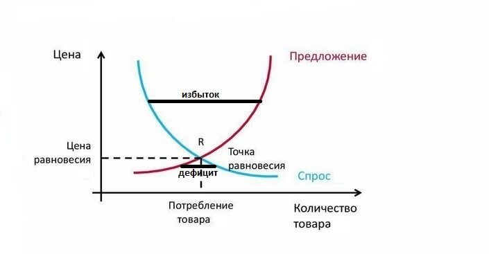
Когда цена и производство растут, то создается переизбыток товаров на рынке. Когда цена и предложение падают, возникает дефицит
Что такое спрос
Спросом называют желание потребителей купить тот или иной продукт. Этот показатель меняется, в зависимости от одного или нескольких факторов:
- цена;
- технологические изменения:
- воздействие государства;
- сезон;
- мода;
- наличие товара на рынке в достаточном количестве;
- число покупателей;
- ценовые прогнозы;
- уровень доходов населения;
- конкуренция в сфере производства товара;
- инфляционные ожидания.
Когда цена на товар снижается, то объем спроса увеличивается. Но бывают и исключения: повышение цен влечет за собой увеличение спроса. У этих явлений есть своё название — эффект Гиффена и парадокс Веблена. В первом случае речь идёт о жизненно важных бюджетных товарах, которые не имеют равноценных заменителей. Во втором — о престижных предметах роскоши. Для этих товаров спрос может расти даже при увеличении их цены.
Пример закона спроса: повышение цены приводит к снижению объёма продаж
Спрос бывает реальным и потенциальным. Реальный показывает, сколько товаров было действительно куплено в тот или иной промежуток времени. Потенциальный демонстрирует, сколько продукции потребители могут приобрести в перспективе. На потенциальный спрос ориентируются производители, планируя объемы производства.
В маркетинге тоже выделяют несколько видов спроса:
- полноценный (предложение соответствует спросу);
- чрезмерный (продавец не может или не успевает удовлетворить потребности покупателей);
- скрытый (есть потребность, но нужной продукции нет в наличии, и покупателям приходится заменять желаемый товар аналогом, отличающимся по качеству или цене);
- отсутствующий (потребители не хотят покупать ту или иную продукцию по разным причинам);
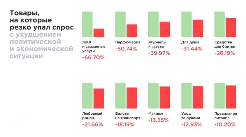
- падающий (когда на рынке появляется более качественный или доступный продукт, потребители отказываются от того товара, которым пользовались раньше).
Спросом можно управлять: делать скидки, проводить акции или рекламные кампании для увеличения продаж. Кампании по увеличению спроса обычно планируются сильно заранее или вовсе имеют сезонный ежегодный характер.

Зимой можно купить летнюю обувь с большими скидками
Что такое предложение
Это желание и готовность продавца реализовать товар. Объем предложения напрямую зависит от объемов производства. Кроме того, на величину предложения влияют и другие факторы:
- себестоимость производства;
- конкуренция;
- прогнозы по цене и уровню потребности;
- сезон;
- новости экономики и политики;
- государственное регулирование;
- налоги;
- цена на аналогичную продукцию других торговых марок.
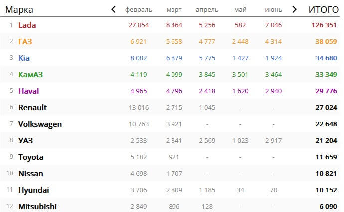
На графике показаны объемы производства автомобилей в РФ в 2022 году. За первые полгода объемы производства машин европейских марок резко снизились. Это привело к падению объемов предложения: сейчас на рынке остались преимущественно отечественные и китайские авто
Когда на рынке возникает избыточное предложение и цены падают, то события неизменно развиваются по одному из двух сценариев (или их комбинации):
- На рынок приходят новые покупатели.
- Производители сокращают объемы производства.
Первый вариант более благоприятен для рынка, но на практике случается редко. Чаще всего производителям приходится сокращать ресурсы, которые затрачиваются на выпуск данной категории товаров.
Так, по данным Росстата, в июле 2022 года объемы производства гречки снизились на 16,7%, по сравнению с июнем. Это связано с тем, что за первые месяцы 2022 года потребители активно покупали крупу и запаслись продукцией на несколько месяцев вперед.
Особенности закона спроса и предложения
Чем выше цена на продукцию, тем продавцу выгоднее сбывать больше товара при прочих равных условиях. Но в качестве сдерживающего рычага выступает спрос: потребителю бывает проще отказаться от покупки, чем платить за нее необоснованную сумму. В этом и заключается взаимосвязь двух величин в законе спроса и предложения.
Цена стремится к такому уровню, где спрос равен предложению. Когда предложение остается неизменным, а спрос растет, возникает дефицит. Соответственно, товары дорожают, так как их не хватает всем покупателям. Если при неизменном предложении спрос падает, снижается и их стоимость: продавцам нужно скорее сбыть излишки.
Когда Apple выводит на рынок новую модель iPhone, стоимость гаджета может достигать сотни тысяч рублей и выше. Но такую цену готов заплатить лишь небольшой процент покупателей, которым важно в числе первых стать обладателями флагманской модели. Спустя несколько недель после старта продаж, производитель постепенно начинает снижать стоимость. К тому моменту, когда будет выпущена следующая модель, цена предыдущей снизится на 30-40% (по сравнению с первоначальной стоимостью).

С момента выпуска 13 модели iPhone прошел год. Изначально цена гаджета составляла около 100 тыс. рублей. Сейчас основное внимание поклонников Apple сконцентрировано на 14 модели: она стоит от 100 тыс. рублей и выше
Кроме того, у Iphone есть модели, которые адаптированы под разные виды спросов. Для потребителей с высокой потребительской способностью представлены более дорогие модели с расширенными функциями. Также существуют заведомо простые и недорогие модели телефонов, доступные широкому кругу покупателей.
Эластичность спроса и предложения
Под эластичностью спроса и предложения понимают то, как эти показатели реагируют на изменение цены. Эластичность спроса показывает, как меняется поведение покупателей, когда продукция дорожает или дешевеет. Если понижение стоимости ведет к увеличению продаж, это значит, что спрос эластичный. Когда потребители не реагируют на удешевление продукции, речь идет о неэластичном спросе.
Товары с эластичным спросом: драгоценности, автомобили, мебель, бытовая техника, деликатесы. Товары с неэластичным спросом: лекарства, топливо для автомобиля, хлеб, соль. Эластичность спроса зависит от степени необходимости товара, наличия аналогов, доли расходов в личном или семейном бюджете (чем чаще человек покупает ту или иную продукцию, тем более предсказуемой будет его реакция на изменение цены).
Антонина Ивановна в июне продавала на рынке клубнику по цене 100 рублей за стакан. К вечеру у женщины осталось всего 2 стакана ягод. Чтобы быстрее уйти домой, продавщица снизила цену до 70 рублей за стакан — продукцию купили в течение 10 минут. Это пример эластичного спроса.
В магазине пиротехники перед новогодними каникулами на 50% вырос объем продаж: все покупали салюты и фейерверки на праздники. После 10 января продажи почти полностью сошли на нет. Руководство снизило цены на 30%, но это не помогло: пиротехника так и осталась нераспроданной. Это пример неэластичного спроса (зависит от степени необходимости для покупателя).
Эластичность предложения, в свою очередь, демонстрирует, как продавцы реагируют на изменение цены: увеличивают или уменьшают объемы продукции на рынке.
От чего зависит эластичность предложения по цене:
- срок хранения товара;
- издержки хранения, в том числе наличие свободных мест на складах;
- вероятность замены компонентов в производстве без потери качества;
- возможность быстро увеличить или уменьшить объемы производства в зависимости от роста или падения цен на продукцию.
Пример неэластичного предложения — билет в кинотеатр. Даже если его цена за неделю вырастет на 100%, продавец не сможет увеличить объем предложения: количество мест в зрительном зале ограничено.
Пример эластичного предложения — мороженое. Если в летние месяцы установилась сильная жара, спрос на продукцию увеличивается в разы даже при том условии, что цена растет. Производители могут быстро увеличить объемы производства и поставить на рынок дополнительные партии продукции. Или наоборот, снизить объемы производства, если лето выдалось холодным и мороженое практически никто не покупает.
Чем больше проходит времени с момента повышения цен или изменения спроса, тем более эластичными становятся спрос и предложение. У покупателей появляется возможность найти замену подорожавшей продукции или изменить свои привычки, а у продавцов — создать новые производственные мощности или избавиться от старых.
Рыночное равновесие: что это и каким оно бывает
Закон спроса и предложения напрямую связан с понятием рыночного равновесия. Это ситуация на рынке, когда объем предложения и спроса совпадают, а на продукцию устанавливается равновесная цена — величина, которая устраивает и продавцов, и покупателей.
Виды рыночного равновесия:
- Устойчивое. Оно означает, что после кратковременного нарушения равновесия на рынке, цены, спрос и предложение быстро восстанавливаются и приходят к предыдущим значениям (или с минимальным отклонением в большую или меньшую сторону).
- Неустойчивое. В этом случае после колебаний на рынке складывается новое соотношение спроса и предложения, а цены существенно отличаются от тех, что были раньше.
В преддверии Нового года традиционно растет спрос на рыбу, икру и морепродукты. Производители наращивают объемы производства, чтобы обеспечить потребность населения в этой продукции. В 2022 году цены на рыбу и икру уже выросли на 10-15%. Но потребители все равно активно покупают деликатесы к праздничному столу. Налицо — пример рыночного равновесия: вырос спрос, продукция подорожала, объемы производства увеличились. Но всех все устраивает. Когда после праздников покупательский интерес спадет, продавцы наверняка будут делать скидки на остатки продукции.
Главные мысли