Как найти эволюту кривой - Исправление недочетов и поиск решений вместе с Examum.ru

Пусть кривая (Gamma) задана натуральным уравнением. Будем предполагать, что в точке (MinGamma), где (overrightarrow{OM}=textbf{r}(s)), существует кривизна (k=k(s)neq 0). Тогда радиус кривизны кривой (Gamma) в точке (M) равен
$$
R=R(s)=frac{1}{k(s)}.label{ref42}
$$

Отложим на главной нормали кривой (Gamma) (рис. 22.9) в направлении главной нормали (nu=nu(s)) отрезок (MN) длиной (R=R(s)) и назовем точку (N) центром кривизны кривой (Gamma) в точке (M). Пусть (overrightarrow{ON}=rho).

Так как (overrightarrow{MN}=R(s)nu(s)), то получаем:
$$
boldsymbol{rho}=textbf{r}(s)+R(s)boldsymbol{nu}(s).label{ref43}
$$

Рис. 22.9

Используя формулу eqref{ref42} и равенство
$$
frac{d^{2}textbf{r}}{ds^{2}}=frac{dtau}{ds}=k(s)boldsymbolnu(s),nonumber
$$
запишем уравнение eqref{ref43} в следующем виде:
$$
boldsymbolrho=textbf{r}(s)+frac{1}{(k(s))^2}frac{d^2textbf{r}}{ds^2}.label{ref44}
$$

Предполагая, что во всех точках кривой (Gamma) кривизна отлична от нуля, построим для каждой точки кривой центр кривизны и назовем множество всех центров кривизны кривой (Gamma) эволютой этой кривой.

Если кривая (Gamma_1) — эволюта кривой (Gamma), то кривую (Gamma) называют эвольвентой кривой (Gamma_1). Уравнение эволюты кривой (Gamma), заданной натуральным уравнением, имеет вид eqref{ref44}.

Если кривая (Gamma) задана уравнением кривой в векторной форме, то уравнение эволюты этой кривой можно получить, заменив в равенстве eqref{ref44} (k) и (displaystylefrac{d^{2}textbf{r}}{ds^{2}}) их выражениями по формулам отсюда и отсюда.

В случае, когда плоская кривая (Gamma) задана уравнением (Gamma={x=x(t),;y=y(t),;alphaleq tleqbeta}), ее кривизна выражается формулой отсюда, а (displaystyle frac{d^2textbf{r}}{ds^2}) — формулой из этого утверждения, где
$$
textbf{r}’=(x’,y’),quad r″=(x″,y″),quad s’=sqrt{(x’)^{2}+(y’)^{2}},quad s″=frac{x’x″+y’y″}{s},nonumber
$$
и поэтому
$$
frac{d^{2}textbf{r}}{ds^{2}}=left(frac{x″}{(s’)^{2}}-frac{x'(x’x″+y’y″)}{(s’)^{4}},;frac{y″}{(s)^{2}}-frac{y'(x’x″+y’y″)}{(s’)^{4}}right)=\=left(displaystyle y’frac{x″y’-x’y″}{((x’)^{2}+(y’)^{2})^{2}},; x’frac{y″x’-y’x″}{((x’)^{2}+(y’)^{2})^{2}}right).nonumber
$$
Если (boldsymbolrho=(xi,eta)), то уравнение eqref{ref44} в координатной форме примет вид
$$
xi=x-y’frac{(x’)^{2}+(y’)^{2}}{x’y″-y’x″},quad eta=y+x’frac{(x’)^{2}+(y’)^{2}}{x’y″-y’x″}.label{ref45}
$$

Равенства eqref{ref45} задают эволюту кривой (Gamma) в координатной форме.

Замечание 1.

Приведем без доказательства физическое истолкование эволюты и эвольвенты. Пусть на эволюту натянута гибкая нерастяжимая нить. Если эту нить развертывать, оставляя все время натянутой, то конец нити опишет эвольвенту. Этим можно объяснить термины эволюта («развертка») и эвольвента («развертывающаяся»).

Пример 1.

Найти эволюту эллипса (x=acos t, y=bsin t).

Решение.

(triangle) В этом случае (x’=-asin t,;y’=bcos t,;x″=acos t,;y″= -bsin t),и формулы eqref{ref45} принимают вид
$$
xi=frac{a^{2}-b^{2}}{a}cos^3 t,quad eta=frac{b^{2}-a^{2}}{b}sin^{3}t.nonumber
$$
Следовательно, эволютой эллипса является астроида. (blacktriangle)

Рис. 22.10

Если плоская кривая задана уравнением (y=f(x)), то уравнения eqref{ref45} записываются в виде
$$
xi=x-frac{1+(f'(x))^{2}}{f″(x)}f'(x),qquad eta=f(x)+frac{1+(f'(x))^{2}}{f″(x)}.label{ref46}
$$

Пример 2.

Найти эволюту параболы (y=ax^{2}).

Решение.

Рис. 22.11

(triangle) Используя формулы eqref{ref46}, где (f(x)=ax^{2}), получаем
$$
xi=x-frac{1+4a^{2}x^{2}}{2a}2ax=-4a^{2}x^{3},qquad eta=ax^{2}+frac{1+4a^{2}x^{2}}{2a}=frac{1}{2a}+3ax^{2}.nonumber
$$
Исключая (x), получаем
$$
xi^{2}=frac{16a}{27}left(eta-frac{1}{2a}right)^{3}.nonumber
$$

Следовательно, эволютой параболы является полукубическая парабола. (blacktriangle)

Источник

=	x− y ‘	1 y’ 2
2) если кривая задана явно, то {=		y ‘ ‘	}.
y 1 y’y‘‘ 2

Определение. Эволюта кривой — это линия, состоящая из всех центров кривизны этой кривой. При этом данная кривая для своей эволюты называется эвольвентой.

Свойства эволюты и эвольвенты

1)Касательная к эволюте является нормалью к эвольвенте.

2)Приращение длины дуги эволюты равно приращению радиуса кривизны эвольвенты.

Пример 1. Найти кривизну и эволюту параболы y=x2. Решение.

а). Найдем кривизну по формуле k =

y»

, подставив сюда

y’ =2 x , y’ ‘=2 :

(1+ (

y’)2 )3/ 2

2 3 /2

Отсюда получаем радиус кривизны: R= 2

1 4 x

1 4 x2 3 /2

б). Координаты центра кривизны вычисляются по формулам:

= x− y’ 1 y ‘ 2

= x−2 x

1 4 x2

= −4 x3

y’ ‘

. Это — параметрические

1 y’ 2

4 x2

{ =

= x

= 1/2 3 x

}

y ‘ ‘

уравнения эволюты. Исключая из

системы параметр x, получим явное

уравнение:

x= − 4 , поэтому

2 2

График эволюты изображен на одном чертеже с параболой.

В точке M0(0,0) кривизна равна 2,

радиус кривизны равен 1/2, центр кривизны (0, 1/2). Геометрически это означает, что в малой окрестности точки M0 парабола лучше всего (из всех окружностей) приближается окружностью x−12 2 y2= 14 . ■

Пример 2. Найти кривизну и эволюту эллипса {xy==abcossintt.,}

Решение. Воспользуемся формулой (1): k =		y»(t)x’(t) − y’(t)x»(t)		.

	( (x’(t))2 + (y’(t))2 )3/ 2
Так как {xy’‘==−bacossintt },	{xy’‘ ‘‘==−−abcossin tt },	и	ab
y»(t)x’(t) − y’(t)x»(t) =	− a sint(− bsin t) + a cost bcost = ab , то k =
	.
(a2 sin2 t + b2 cos2 t)3 2

Координаты центра кривизны вычисляются по формулам:

= a cos t−b cost a2 sin2 t b2 cos2 t ab

= b sin t−a sin t a2 sin2 t b2 cos2 t ab

	=	x −y’	x ‘ 2 y ‘ 2
x’ y’ ‘−x ‘ ‘ y’
{
=	y x’	x ‘ 2 y ‘ 2
x’ y’ ‘−x ‘ ‘ y’

Это — параметрические уравнения эволюты. Для исключения из системы параметра t, преобразуем её:

a 2 /3	=	a2 −b2 2/3 cos2 t	},
{b 2 /3	=	b2−a2 2 /3 sin2 t	откуда, складывая
уравнения, получаем неявное уравнение эволюты:
(aξ )23 + (bη )23	= (b2 − a2 )23 — это асторида.
Вершины астроиды:
при	=0	=± a2−b2 ;
				b
при	=0	=±	a2 −b2	.

				a
Если a = 4, b = 2, то вершины астроиды: 0,±6 ,	±3,0 . ■

=	a2−b2 cos3 t	}.
	a
=	b2−b a2 sin3 t
	7
	5
	3
	1

-5 -4 -3 -2 —11 0 1 2 3 4 5

-3

-5

-7

Источник

Содержание

Соприкасающаяся окружность. Эволюта, эвольвента

Разбор ДЗ

2. Найти кривизну и кручение кривой, заданной в неявном виде: $-x^2+y^2+z^2=1$, $-x^2+2y-z=0$ в точке $M(1,,1,,1)$.

Ответ: $k=displaystylefrac{sqrt{6}}{6}$, $varkappa=1$.

3. Доказать, что кривая $x=1+2t+t^2, y=2-5t+t^2, z=1+t^2$~ — плоская. Найти уравнение плоскости, в которой лежит эта кривая.

Ответ: $varkappa=0$, $5x+2y-7z-2=0$.

Краткие теоретические сведения

Соприкосновение $k$-того порядка

Две кривые
$$ gamma_1: vec{r}_1=vec{r}_1(t),, mbox{и} ,, gamma_2: vec{r}_2=vec{r}_2(t) $$
имеют в общей точке $M_0$ соприкосновение (касание) $k$-того порядка, если в этой точке:
begin{equation*}
frac{dvec{r}_1}{dt}=frac{dvec{r}_2}{dt}, ldots, frac{d^kvec{r}_1}{dt^k}=frac{d^kvec{r}_2}{dt^k},, frac{d^{k+1}vec{r}_1}{dt^k}neqfrac{d^{k+1}vec{r}_2}{dt^k}.
end{equation*}

Для неявно заданных кривых — см. формулы в Феденко.

Касательная кривой имеет в точке касания имеет соприкосновение первого порядка.

Соприкасающаяся окружность плоской кривой

Пусть $gamma$ — плоская кривая, $M_0 (t=t_0)$ — точка на ней.

Окружность, проходящая через точку $M_0$, называется соприкасающейся окружностью кривой $gamma$ в точке $M_0$, если кривая в этой точке с окружностью имеет соприкосновение второго порядка (не ниже второго порядка).

Центр соприкасающейся окружности называют центром кривизны кривой в заданной точке.

Центр окружности лежит на нормали к кривой. Радиус окружности (радиус кривизны) есть величина, обратная кривизне этой кривой в заданной точке $M_0$:
$$ R=1/k(t_0).$$

Эволюта и эвольвента

Эволютой плоской кривой называется огибающая ее нормалей.

Эволюта это геометрическое место центров кривизны плоской кривой.

Уравнение эволюты:
begin{equation*}
X = x-y’frac{(x’)^2+(y’)^2}{x’y»-x»y’}, ,, Y= y+x’frac{(x’)^2+(y’)^2}{x’y»-x»y’}.
end{equation*}

Эвольвентой плоской кривой $gamma$ называется такая кривая $Gamma$ по отношению к которой $gamma$ является эволютой.

Уравнение эвольвенты:
begin{gather*}
R = vec{r(}t)-frac{vec{r’}(t)}{sqrt{(vec{r’})^2}}intsqrt{(vec{r’}(t))^2},dt.
end{gather*}

Решение задач

Задача 1 (Феденко № 179)

Докажите, что линии
begin{equation*}
y_1=mbox{sin},x, ,, y_2=x^4-frac16x^3+x.
end{equation*}
имеют в начале координат касание третьего порядка

Решение задачи 1

begin{equation*}
begin{split}
&y_1(0)=y_2(0)=0, \
&y’_1(0)=y’_2(0)=1, \
&y»_1(0)= y»_2(0)=0, \
&y»’_1(0)=y»’_2(0)=-1, \
&y_1^{(4)}(0)=0neq y_2^{(4)}(0)=24. \
&end{split}
end{equation*}

Задача 2 (Феденко №369)

Напишите уравнение соприкасающейся окружности линии $y=mbox{sin},x$ в точке $Aleft(frac{pi}{2}; 1right)$.

Решение задачи 2

Радиус соприкасающейся плоскости $R=displaystylefrac{1}{k}$. Найдем кривизну для заданной кривой:
begin{equation*}
k = displaystylefrac{|y»|}{left(1+(y’)^2right)^{3/2}}=frac{mbox{sin},x}{(1+mbox{cos}^2,x)^{3/2}}.
end{equation*}
begin{equation*}
kleft(frac{pi}{2}right)=1 ,, Rightarrow ,, R=1.
end{equation*}
Учитывая, что окружность касается синусоиды в точке $Aleft(displaystylefrac{pi}{2}; 1right)$, радиус окружности равен $1$ и центр окружности лежит на нормали, проведенной в точке касания, получаем следующее уравнение:
begin{equation*}
left(x-displaystylefrac{pi}{2}right)^2+y^2=1.
end{equation*}

Задача 3 (Феденко №391)

Составьте уравнения и начертите эволюту кривой
begin{equation*}
x=aleft(mbox{ln},mbox{tg},left(displaystylefrac{t}{2}right)+mbox{cos},tright), ,, y = a,mbox{sin},t.
end{equation*}

Решение задачи 3

Находим производные.
begin{equation*}
begin{split}
x’&=aleft(frac{1}{mbox{sin},t}-mbox{sin},tright)=afrac{mbox{cos}^2t}{mbox{sin},t},\
x»&=-a,mbox{cos},tleft(1+frac{1}{mbox{sin}^2,t}right),\
y’&=a,mbox{cos},t, quad y»=-a,mbox{sin},t.
end{split}
end{equation*}
begin{equation*}
begin{split}
&(x’)^2+(y’)^2=a^2mbox{ctg}^2,t,\
&x’y»-x»y’=a^2mbox{ctg}^2,t.
end{split}
end{equation*}

Получаем уравнения эволюты:
begin{equation*}
begin{split}
&X= x(t)-a,mbox{cos},tcdot1,,, Y= y(t)+a,displaystylefrac{mbox{cos}^2t}{mbox{sin},t}cdot1.\
&X = a,mbox{ln},mbox{tg},left(displaystylefrac{t}{2}right), ,, Y= displaystylefrac{a}{mbox{sin},t}.
end{split}
end{equation*}

Задача 4 (Феденко №397)

Составьте уравнения эвольвент окружности $x^2+y^2=a^2$ и сделайте рисунок.

Решение задачи 4

Запишем параметрическое уравнение окружности:
begin{equation*}
x=a,mbox{cos},t, ,, y=a,mbox{sin},t.
end{equation*}

begin{gather*}
vec{r}(t)={a,mbox{cos},t,,,a,mbox{sin},t},\
vec{r’}(t)={-a,mbox{sin},t,,,a,mbox{cos},t},\
(vec{r’}(t))^2=a^2,\
intsqrt{(vec{r’}(t))^2},dt = int a,dt = at+C.
end{gather*}

Уравнения эвольвент:
begin{equation*}
begin{array}{ccc}
X&=&a,mbox{cos},t + (at+C),mbox{sin},t,\
Y&=&a,mbox{sin},t — (at+C),mbox{cos},t.\
end{array}
end{equation*}

diffgeom/seminar4.txt

· Последние изменения: 2021/03/28 21:00 —

nvr

Источник

From Wikipedia, the free encyclopedia

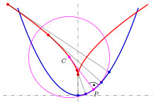
The evolute of a curve (blue parabola) is the locus of all its centers of curvature (red).

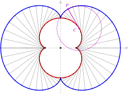
The evolute of a curve (in this case, an ellipse) is the envelope of its normals.

In the differential geometry of curves, the evolute of a curve is the locus of all its centers of curvature. That is to say that when the center of curvature of each point on a curve is drawn, the resultant shape will be the evolute of that curve. The evolute of a circle is therefore a single point at its center.^[1] Equivalently, an evolute is the envelope of the normals to a curve.

The evolute of a curve, a surface, or more generally a submanifold, is the caustic of the normal map. Let M be a smooth, regular submanifold in Rⁿ. For each point p in M and each vector v, based at p and normal to M, we associate the point p + v. This defines a Lagrangian map, called the normal map. The caustic of the normal map is the evolute of M.^[2]

Evolutes are closely connected to involutes: A curve is the evolute of any of its involutes.

History[edit]

Apollonius (c. 200 BC) discussed evolutes in Book V of his Conics. However, Huygens is sometimes credited with being the first to study them (1673). Huygens formulated his theory of evolutes sometime around 1659 to help solve the problem of finding the tautochrone curve, which in turn helped him construct an isochronous pendulum. This was because the tautochrone curve is a cycloid, and the cycloid has the unique property that its evolute is also a cycloid. The theory of evolutes, in fact, allowed Huygens to achieve many results that would later be found using calculus.^[3]

Evolute of a parametric curve[edit]

If ${displaystyle {vec {x}}={vec {c}}(t),;tin [t_{1},t_{2}]}$ is the parametric representation of a regular curve in the plane with its curvature nowhere 0 and its curvature radius and the unit normal pointing to the curvature center, then

describes the evolute of the given curve.

For ${displaystyle {vec {c}}(t)=(x(t),y(t))^{mathsf {T}}}$ and ${displaystyle {vec {E}}=(X,Y)^{mathsf {T}}}$ one gets

${displaystyle X(t)=x(t)-{frac {y'(t){Big (}x'(t)^{2}+y'(t)^{2}{Big )}}{x'(t)y''(t)-x''(t)y'(t)}}}$

and

${displaystyle Y(t)=y(t)+{frac {x'(t){Big (}x'(t)^{2}+y'(t)^{2}{Big )}}{x'(t)y''(t)-x''(t)y'(t)}}.}$

Properties of the evolute[edit]

The normal at point P is the tangent at the curvature center C.

In order to derive properties of a regular curve it is advantageous to use the arc length of the given curve as its parameter, because of and (see Frenet–Serret formulas). Hence the tangent vector of the evolute is:

From this equation one gets the following properties of the evolute:

Proof of the last property:
Let be at the section of consideration. An involute of the evolute can be described as follows:

${displaystyle {vec {C}}_{0}={vec {E}}-{frac {{vec {E}}'}{left|{vec {E}}'right|}}left(int _{0}^{s}left|{vec {E}}'(w)right|mathrm {d} w+l_{0}right),}$

where l_0 is a fixed string extension (see Involute of a parameterized curve ).
With and one gets

${displaystyle {vec {C}}_{0}={vec {c}}+rho {vec {n}}-{vec {n}}left(int _{0}^{s}rho '(w);mathrm {d} w;+l_{0}right)={vec {c}}+(rho (0)-l_{0});{vec {n}},.}$

That means: For the string extension ${displaystyle l_{0}=rho (0)}$ the given curve is reproduced.

Parallel curves have the same evolute.

Proof: A parallel curve with distance off the given curve has the parametric representation ${displaystyle {vec {c}}_{d}={vec {c}}+d{vec {n}}}$ and the radius of curvature ${displaystyle rho _{d}=rho -d}$ (see parallel curve). Hence the evolute of the parallel curve is

${displaystyle {vec {E}}_{d}={vec {c}}_{d}+rho _{d}{vec {n}}={vec {c}}+d{vec {n}}+(rho -d){vec {n}}={vec {c}}+rho {vec {n}}={vec {E}};.}$

Examples[edit]

Evolute of a parabola[edit]

For the parabola with the parametric representation $(t,t^{2})$ one gets from the formulae above the equations:

${displaystyle X=cdots =-4t^{3}}$

${displaystyle Y=cdots ={frac {1}{2}}+3t^{2},,}$

which describes a semicubic parabola

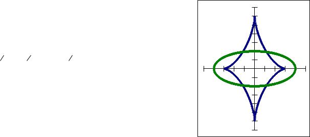
Evolute (red) of an ellipse

Evolute of an ellipse[edit]

For the ellipse with the parametric representation one gets:^[5]

${displaystyle X=cdots ={frac {a^{2}-b^{2}}{a}}cos ^{3}t}$

${displaystyle Y=cdots ={frac {b^{2}-a^{2}}{b}}sin ^{3}t;.}$

These are the equations of a non symmetric astroid.
Eliminating parameter leads to the implicit representation

${displaystyle (aX)^{tfrac {2}{3}}+(bY)^{tfrac {2}{3}}=(a^{2}-b^{2})^{tfrac {2}{3}} .}$

Cycloid (blue), its osculating circle (red) and evolute (green).

Evolute of a cycloid[edit]

For the cycloid with the parametric representation the evolute will be:^[6]

which describes a transposed replica of itself.

The evolute of the large nephroid (blue) is the small nephroid (red).

Evolutes of some curves[edit]

The evolute

of a parabola is a semicubic parabola (see above),
of an ellipse is a non symmetric astroid (see above),
of a line is an ideal point,
of a nephroid is a nephroid (half as large, see diagram),
of an astroid is an astroid (twice as large),
of a cardioid is a cardioid (one third as large),
of a circle is its center,
of a deltoid is a deltoid (three times as large),
of a cycloid is a congruent cycloid,
of a logarithmic spiral is the same logarithmic spiral,
of a tractrix is a catenary.

Radial curve[edit]

A curve with a similar definition is the radial of a given curve. For each point on the curve take the vector from the point to the center of curvature and translate it so that it begins at the origin. Then the locus of points at the end of such vectors is called the radial of the curve. The equation for the radial is obtained by removing the x and y terms from the equation of the evolute. This produces

${displaystyle (X,Y)=left(-y'{frac {{x'}^{2}+{y'}^{2}}{x'y''-x''y'}};,;x'{frac {{x'}^{2}+{y'}^{2}}{x'y''-x''y'}}right).}$

References[edit]

^ Weisstein, Eric W. «Circle Evolute». MathWorld.
^ Arnold, V. I.; Varchenko, A. N.; Gusein-Zade, S. M. (1985). The Classification of Critical Points, Caustics and Wave Fronts: Singularities of Differentiable Maps, Vol 1. Birkhäuser. ISBN 0-8176-3187-9.
^ Yoder, Joella G. (2004). Unrolling Time: Christiaan Huygens and the Mathematization of Nature. Cambridge University Press.
^ Ghys, Étienne; Tabachnikov, Sergei; Timorin, Vladlen (2013). «Osculating curves: around the Tait-Kneser theorem». The Mathematical Intelligencer. 35 (1): 61–66. arXiv:1207.5662. doi:10.1007/s00283-012-9336-6. MR 3041992.
^ R.Courant: Vorlesungen über Differential- und Integralrechnung. Band 1, Springer-Verlag, 1955, S. 268.
^ Weisstein, Eric W. «Cycloid Evolute». MathWorld.

Weisstein, Eric W. «Evolute». MathWorld.
Sokolov, D.D. (2001) [1994], «Evolute», Encyclopedia of Mathematics, EMS Press
Yates, R. C.: A Handbook on Curves and Their Properties, J. W. Edwards (1952), «Evolutes.» pp. 86ff
Evolute on 2d curves.

Источник

Эволюта

Материал из Большого Справочника

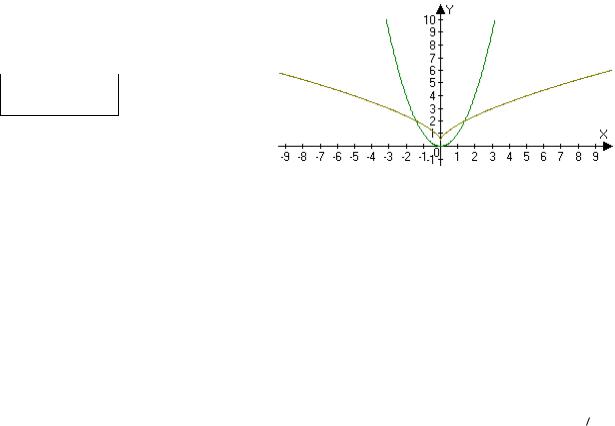
Синим цветом показана гипербола. Зелёным цветом — эволюта правой ветви этой гиперболы (эволюта левой ветви вне рисунка. Красным цветом показана окружность, соответствующая кривизне гиперболы в её вершине)

Эволюта плоской кривой — геометрическое место точек, являющихся центрами кривизны кривой.
По отношению к своей эволюте любая кривая является эвольвентой.

Уравнения

Если линия задана параметрическими уравнениями , то её эволюта имеет уравнение:

${displaystyle X=x(t)-y'{frac {x'^{2}+y'^{2}}{x'y''-x''y'}},}$

${displaystyle Y=y(t)+x'{frac {x'^{2}+y'^{2}}{x'y''-x''y'}}}$

В частности, если является натуральным параметром кривой , то её эволюта может быть задана^[1] уравнением:

${displaystyle {vec {r}}(t)+{frac {1}{k(t)}}{vec {n}}(t)}$

где — единичный вектор нормали кривой, направленный в сторону центра кривизны, — кривизна.

Примеры

Вытянутая астроида как эволюта эллипса

Вытянутая астроида

${displaystyle x={frac {a^{2}-b^{2}}{a}}cos ^{3}t,quad y={frac {b^{2}-a^{2}}{b}}sin ^{3}t}$

является эволютой эллипса

${frac {x^{2}}{a^{2}}}+{frac {y^{2}}{b^{2}}}=1$

Эволюта астроиды подобна ей, но вдвое больше неё и повёрнута относительно неё на 45°.
Эволюта циклоиды является циклоидой, конгруэнтной исходной, а именно — параллельно сдвинутой так, что вершины переходят в «острия».
- Эти свойства открыты Христианом Гюйгенсом; они были им использованы для создания точных механических часов собственная частота маятника в которых не зависит от амплитуды колебаний.

См. также

Эвольвента
Параллельная кривая
Соприкасающаяся окружность

Примечания

↑ Эволюта — статья из Математической энциклопедии. Д. Д. Соколов

Литература

Д. А. Граве. Дифференциальное исчисление // Энциклопедический словарь Брокгауза и Ефрона : в 86 т. (82 т. и 4 доп.). — СПб., 1890—1907.
В. Бляшке. Диференциальная геометрия и геометрические основы теории относительности Эйнштейна / М. Я. Выгодский (перевод с немецкого). — М.: ОНТИ, 1935. — 331 с.

Источник