Как найти функцию плотности вероятности случайной величины

Плотность распределения вероятностей непрерывной случайной величины

Краткая теория
Примеры решения задач
Задачи контрольных и самостоятельных работ

Краткая теория

Ранее
непрерывная случайная величина задавалась с помощью функции распределения. Этот
способ задания не является единственным. Непрерывную случайную величину можно
также задать, используя другую функцию, которую называют плотностью
распределения или плотностью вероятности (иногда ее называют дифференциальной
функцией).

Плотностью распределения вероятностей непрерывной случайной величины

называют функцию

– первую производную от функции распределения

Из этого определения следует, что
функция распределения является первообразной для плотности распределения.

Заметим, что для описания
распределения вероятностей дискретной случайной величины плотность
распределения неприменима.

Зная плотность распределения, можно
вычислить вероятность того, что непрерывная случайная величина примет значение,
принадлежащее заданному интервалу.

Вероятность того, что непрерывная
случайная величина

примет
значение, принадлежащее интервалу

равна
определенному интегралу от плотности распределения, взятому в пределах от

до

Геометрически полученный результат
можно истолковать так: вероятность того, что непрерывная случайная величина
примет значение, принадлежащее интервалу

, равна площади криволинейной трапеции, ограниченной
осью

, кривой распределения

и прямыми

В частности, если

– четная
функция и концы интервала симметричны относительно начала координат, то:

Зная плотность распределения

можно найти
функцию распределения

по формуле:

Свойства плотности распределения

Свойство 1.

Плотность
распределения – неотрицательная функция:

Свойство 2.

Несобственный
интеграл от плотности распределения в пределах от

до

равен единице:

Смежные темы решебника:

Дискретная случайная величина
Непрерывная случайная величина
Интегральная функция распределения вероятностей

Примеры решения задач

Пример 1

Задана
плотность распределения вероятностей f(x) непрерывной случайной
величины X. Требуется:

1)
определить коэффициент A;

2) найти
функцию распределения F(x);

3)
схематично построить графики F(x) и f(x);

4) найти
математическое ожидание и дисперсию X;

5) найти
вероятность того, что X примет значение из
интервала (α,β):

α=1; β=1.7

Решение

На сайте можно заказать решение контрольной или самостоятельной работы, домашнего задания, отдельных задач. Для этого вам нужно только связаться со мной:

ВКонтакте
WhatsApp
Telegram

Мгновенная связь в любое время и на любом этапе заказа. Общение без посредников. Удобная и быстрая оплата переводом на карту СберБанка. Опыт работы более 25 лет.

Подробное решение в электронном виде (docx, pdf) получите точно в срок или раньше.

1)
Постоянный параметр

найдем из
свойства плотности вероятности:

В
нашем случае эта формула имеет вид:

Получаем:

2)
Функцию распределения

найдем из
формулы:

Учитывая
свойства

, сразу можем
отметить, что:

Остается
найти выражение для

, когда

принадлежит
интервалу

Получаем:

3) Построим графики

График плотности распределения

График функции распределения

4)
Математическое ожидание находим по формуле:

Для
нашего примера:

Дисперсию
можно найти по формуле:

5)
Вероятность того, что случайная величина примет значение из интервала

Пример 2

Плотность
распределения вероятности непрерывной случайной величины равна

, x∈(0,∞). Найти нормировочный множитель C,
математическое ожидание M(X) и дисперсию D(X).

Решение

Нормировочный множитель

найдем из
свойства плотности вероятности:

В
нашем случае эта формула имеет вид:

Плотность
вероятности:

Математическое
ожидание находим по формуле:

Для
нашего примера:

Дисперсию
можно найти по формуле:

Пример 3

Непрерывная
случайная величина

имеет плотность распределения:

Найти
величину a, вероятность P(X<0) и математическое
ожидание X.

Решение

ВКонтакте
WhatsApp
Telegram

Подробное решение в электронном виде (docx, pdf) получите точно в срок или раньше.

Постоянный
параметр

найдем из
свойства плотности вероятности:

В
нашем случае эта формула имеет вид:

Плотность
вероятности имеет вид:

Вероятность:

Математическое
ожидание находим по формуле:

Для
нашего примера:

Задачи контрольных и самостоятельных работ

Задача 1

Плотность
распределения непрерывной случайной величины X имеет вид:

Найти:

а)
параметр a;

б)
функцию распределения F(x);

в)
вероятность попадания случайной величины X в интервал (6.5; 11);

г)
математическое ожидание M(X) и дисперсию D(X);

Построить
график функций f(x) и F(x).

Задача 2

Задана
функция распределения непрерывной случайной величины:

Найти и
построить график функции плотности распределения вероятностей.

Задача 3

Случайная
величина X задана функцией распределения F(x).
Найти плотность распределения вероятностей, математическое ожидание и дисперсию
случайной величины. Построить график функции
F(x).

Задача 4

Задана
плотность вероятности f(x) или функции распределения
непрерывной случайной величины X. Найти a, M[X], D[X], P(α<x<β).

α=1,β=2

ВКонтакте
WhatsApp
Telegram

Подробное решение в электронном виде (docx, pdf) получите точно в срок или раньше.

Задача 5

Непрерывная
случайная величина

задана плотностью распределения вероятностей.

Требуется
найти:

— функцию
распределения вероятностей;

—
математическое ожидание;

—
дисперсию;

— среднее
квадратическое отклонение;

— вероятность
того, что случайная величина отклонится от своего математического ожидания не
более, чем на одну четвертую длины всего интервала возможных значений этой
величины;

—
построить графики функции распределения и плотности распределения вероятностей.

Задача 6

Случайная
величина X равномерно распределена на интервале (2;7).
Составить f(x),F(x), построить графики. Найти
M(X),D(X).

Задача 7

Случайная
величина X~N(a,σ)

a=25;
σ=4; α=13; β=30; δ=0.1.

Требуется:

—
составить функцию плотности распределения и построить ее график;

— найти
вероятность того, что случайная величина в результате испытания примет
значение, принадлежащее интервалу (α; β);

— найти
вероятность того, что абсолютная величина отклонения значений случайной
величины от ее математического ожидания не превысит δ.

Задача 8

Плотность
вероятности непрерывной случайной величины ξ задана следующим выражением:

Найти
постоянную C, функцию распределения Fξ (x), математическое
ожидание и дисперсию Dξ случайной величины ξ.

ВКонтакте
WhatsApp
Telegram

Подробное решение в электронном виде (docx, pdf) получите точно в срок или раньше.

Задача 9

Случайная
величина X задана функцией распределения вероятностей F(x).

Требуется:

1. Найти
функцию плотности распределения f(x).

2. Найти M(X).

3. Найти
вероятность P(α<X<β)

4.
Построить графики f(x) и F(x).

α=2, β=4.5

Задача 10

Найти
функцию плотности нормально распределенной случайной величины X и
постройте ее график, зная M(X) и D(X).

M(X)=-1; D(X)=8

Задача 11

Случайная
величина X задана интегральной F(x) или дифференциальной f(x)
функцией. Требуется:

а) найти
параметр C;

б) при
заданной интегральной функции F(x) найти дифференциальную функцию f(x), а при
заданной дифференциальной функции f(x) найти интегральную функцию F(x);

в)
построить графики функций F(x) и f(x);

г) найти
математическое ожидание M(X), дисперсию D(X) и
среднее квадратическое отклонение σ(x);

д)
вычислить вероятность попадания в интервал P(a≤x≤b)

е)
определить, квантилем какого порядка является точка xp;

ж)
вычислить квантиль порядка p

a=π/4; b=π/3; xp=π/2; p=0.75

Краткая теория
Примеры решения задач
Задачи контрольных и самостоятельных работ

Источник

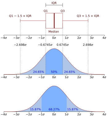
Geometric visualisation of the mode, median and mean of an arbitrary unimodal probability density function.^[1]

In probability theory, a probability density function (PDF), or density of an absolutely continuous random variable, is a function whose value at any given sample (or point) in the sample space (the set of possible values taken by the random variable) can be interpreted as providing a relative likelihood that the value of the random variable would be equal to that sample.^[2]^[3] Probability density is the probability per unit length, in other words, while the absolute likelihood for a continuous random variable to take on any particular value is 0 (since there is an infinite set of possible values to begin with), the value of the PDF at two different samples can be used to infer, in any particular draw of the random variable, how much more likely it is that the random variable would be close to one sample compared to the other sample.

In a more precise sense, the PDF is used to specify the probability of the random variable falling within a particular range of values, as opposed to taking on any one value. This probability is given by the integral of this variable’s PDF over that range—that is, it is given by the area under the density function but above the horizontal axis and between the lowest and greatest values of the range. The probability density function is nonnegative everywhere, and the area under the entire curve is equal to 1.

The terms probability distribution function and probability function have also sometimes been used to denote the probability density function. However, this use is not standard among probabilists and statisticians. In other sources, «probability distribution function» may be used when the probability distribution is defined as a function over general sets of values or it may refer to the cumulative distribution function, or it may be a probability mass function (PMF) rather than the density. «Density function» itself is also used for the probability mass function, leading to further confusion.^[4] In general though, the PMF is used in the context of discrete random variables (random variables that take values on a countable set), while the PDF is used in the context of continuous random variables.

Example[edit]

Suppose bacteria of a certain species typically live 4 to 6 hours. The probability that a bacterium lives exactly 5 hours is equal to zero. A lot of bacteria live for approximately 5 hours, but there is no chance that any given bacterium dies at exactly 5.00… hours. However, the probability that the bacterium dies between 5 hours and 5.01 hours is quantifiable. Suppose the answer is 0.02 (i.e., 2%). Then, the probability that the bacterium dies between 5 hours and 5.001 hours should be about 0.002, since this time interval is one-tenth as long as the previous. The probability that the bacterium dies between 5 hours and 5.0001 hours should be about 0.0002, and so on.

In this example, the ratio (probability of dying during an interval) / (duration of the interval) is approximately constant, and equal to 2 per hour (or 2 hour⁻¹). For example, there is 0.02 probability of dying in the 0.01-hour interval between 5 and 5.01 hours, and (0.02 probability / 0.01 hours) = 2 hour⁻¹. This quantity 2 hour⁻¹ is called the probability density for dying at around 5 hours. Therefore, the probability that the bacterium dies at 5 hours can be written as (2 hour⁻¹) dt. This is the probability that the bacterium dies within an infinitesimal window of time around 5 hours, where dt is the duration of this window. For example, the probability that it lives longer than 5 hours, but shorter than (5 hours + 1 nanosecond), is (2 hour⁻¹)×(1 nanosecond) ≈ 6×10⁻¹³ (using the unit conversion 3.6×10¹² nanoseconds = 1 hour).

There is a probability density function f with f(5 hours) = 2 hour⁻¹. The integral of f over any window of time (not only infinitesimal windows but also large windows) is the probability that the bacterium dies in that window.

Absolutely continuous univariate distributions[edit]

A probability density function is most commonly associated with absolutely continuous univariate distributions. A random variable has density f_X , where f_X is a non-negative Lebesgue-integrable function, if:

${displaystyle Pr[aleq Xleq b]=int _{a}^{b}f_{X}(x),dx.}$

Hence, if $F_{X}$ is the cumulative distribution function of , then:

${displaystyle F_{X}(x)=int _{-infty }^{x}f_{X}(u),du,}$

and (if f_X is continuous at )

${displaystyle f_{X}(x)={frac {d}{dx}}F_{X}(x).}$

Intuitively, one can think of ${displaystyle f_{X}(x),dx}$ as being the probability of falling within the infinitesimal interval .

Formal definition[edit]

(This definition may be extended to any probability distribution using the measure-theoretic definition of probability.)

A random variable with values in a measurable space (usually $mathbb {R} ^{n}$ with the Borel sets as measurable subsets) has as probability distribution the measure X_∗P on : the density of with respect to a reference measure on is the Radon–Nikodym derivative:

${displaystyle f={frac {dX_{*}P}{dmu }}.}$

That is, f is any measurable function with the property that:

${displaystyle Pr[Xin A]=int _{X^{-1}A},dP=int _{A}f,dmu }$

for any measurable set

Discussion[edit]

In the continuous univariate case above, the reference measure is the Lebesgue measure. The probability mass function of a discrete random variable is the density with respect to the counting measure over the sample space (usually the set of integers, or some subset thereof).

It is not possible to define a density with reference to an arbitrary measure (e.g. one can’t choose the counting measure as a reference for a continuous random variable). Furthermore, when it does exist, the density is almost unique, meaning that any two such densities coincide almost everywhere.

Further details[edit]

Unlike a probability, a probability density function can take on values greater than one; for example, the uniform distribution on the interval [0, 1/2] has probability density f(x) = 2 for 0 ≤ x ≤ 1/2 and f(x) = 0 elsewhere.
The standard normal distribution has probability density

${displaystyle f(x)={frac {1}{sqrt {2pi }}},e^{-x^{2}/2}.}$

If a random variable X is given and its distribution admits a probability density function f, then the expected value of X (if the expected value exists) can be calculated as

${displaystyle operatorname {E} [X]=int _{-infty }^{infty }x,f(x),dx.}$

Not every probability distribution has a density function: the distributions of discrete random variables do not; nor does the Cantor distribution, even though it has no discrete component, i.e., does not assign positive probability to any individual point.

A distribution has a density function if and only if its cumulative distribution function F(x) is absolutely continuous. In this case: F is almost everywhere differentiable, and its derivative can be used as probability density:

${displaystyle {frac {d}{dx}}F(x)=f(x).}$

If a probability distribution admits a density, then the probability of every one-point set {a} is zero; the same holds for finite and countable sets.

Two probability densities f and g represent the same probability distribution precisely if they differ only on a set of Lebesgue measure zero.

In the field of statistical physics, a non-formal reformulation of the relation above between the derivative of the cumulative distribution function and the probability density function is generally used as the definition of the probability density function. This alternate definition is the following:

If dt is an infinitely small number, the probability that X is included within the interval (t, t + dt) is equal to f(t) dt, or:

Link between discrete and continuous distributions[edit]

It is possible to represent certain discrete random variables as well as random variables involving both a continuous and a discrete part with a generalized probability density function using the Dirac delta function. (This is not possible with a probability density function in the sense defined above, it may be done with a distribution.) For example, consider a binary discrete random variable having the Rademacher distribution—that is, taking −1 or 1 for values, with probability 1⁄2 each. The density of probability associated with this variable is:

${displaystyle f(t)={frac {1}{2}}(delta (t+1)+delta (t-1)).}$

More generally, if a discrete variable can take n different values among real numbers, then the associated probability density function is:

${displaystyle f(t)=sum _{i=1}^{n}p_{i},delta (t-x_{i}),}$

where $x_{1},ldots ,x_{n}$ are the discrete values accessible to the variable and are the probabilities associated with these values.

This substantially unifies the treatment of discrete and continuous probability distributions. The above expression allows for determining statistical characteristics of such a discrete variable (such as the mean, variance, and kurtosis), starting from the formulas given for a continuous distribution of the probability.

Families of densities[edit]

It is common for probability density functions (and probability mass functions) to be parametrized—that is, to be characterized by unspecified parameters. For example, the normal distribution is parametrized in terms of the mean and the variance, denoted by and $sigma ^{2}$ respectively, giving the family of densities

${displaystyle f(x;mu ,sigma ^{2})={frac {1}{sigma {sqrt {2pi }}}}e^{-{frac {1}{2}}left({frac {x-mu }{sigma }}right)^{2}}.}$

Different values of the parameters describe different distributions of different random variables on the same sample space (the same set of all possible values of the variable); this sample space is the domain of the family of random variables that this family of distributions describes. A given set of parameters describes a single distribution within the family sharing the functional form of the density. From the perspective of a given distribution, the parameters are constants, and terms in a density function that contain only parameters, but not variables, are part of the normalization factor of a distribution (the multiplicative factor that ensures that the area under the density—the probability of something in the domain occurring— equals 1). This normalization factor is outside the kernel of the distribution.

Since the parameters are constants, reparametrizing a density in terms of different parameters to give a characterization of a different random variable in the family, means simply substituting the new parameter values into the formula in place of the old ones.

Densities associated with multiple variables[edit]

For continuous random variables X₁, …, X_n, it is also possible to define a probability density function associated to the set as a whole, often called joint probability density function. This density function is defined as a function of the n variables, such that, for any domain D in the n-dimensional space of the values of the variables X₁, …, X_n, the probability that a realisation of the set variables falls inside the domain D is

${displaystyle Pr left(X_{1},ldots ,X_{n}in Dright)=int _{D}f_{X_{1},ldots ,X_{n}}(x_{1},ldots ,x_{n}),dx_{1}cdots dx_{n}.}$

If F(x₁, …, x_n) = Pr(X₁ ≤ x₁, …, X_n ≤ x_n) is the cumulative distribution function of the vector (X₁, …, X_n), then the joint probability density function can be computed as a partial derivative

${displaystyle f(x)=left.{frac {partial ^{n}F}{partial x_{1}cdots partial x_{n}}}right|_{x}}$

Marginal densities[edit]

For i = 1, 2, …, n, let f_{X_i}(x_i) be the probability density function associated with variable X_i alone. This is called the marginal density function, and can be deduced from the probability density associated with the random variables X₁, …, X_n by integrating over all values of the other n − 1 variables:

${displaystyle f_{X_{i}}(x_{i})=int f(x_{1},ldots ,x_{n}),dx_{1}cdots dx_{i-1},dx_{i+1}cdots dx_{n}.}$

Independence[edit]

Continuous random variables X₁, …, X_n admitting a joint density are all independent from each other if and only if

${displaystyle f_{X_{1},ldots ,X_{n}}(x_{1},ldots ,x_{n})=f_{X_{1}}(x_{1})cdots f_{X_{n}}(x_{n}).}$

Corollary[edit]

If the joint probability density function of a vector of n random variables can be factored into a product of n functions of one variable

${displaystyle f_{X_{1},ldots ,X_{n}}(x_{1},ldots ,x_{n})=f_{1}(x_{1})cdots f_{n}(x_{n}),}$

(where each f_i is not necessarily a density) then the n variables in the set are all independent from each other, and the marginal probability density function of each of them is given by

${displaystyle f_{X_{i}}(x_{i})={frac {f_{i}(x_{i})}{int f_{i}(x),dx}}.}$

Example[edit]

This elementary example illustrates the above definition of multidimensional probability density functions in the simple case of a function of a set of two variables. Let us call a 2-dimensional random vector of coordinates (X, Y): the probability to obtain in the quarter plane of positive x and y is

${displaystyle Pr left(X>0,Y>0right)=int _{0}^{infty }int _{0}^{infty }f_{X,Y}(x,y),dx,dy.}$

Function of random variables and change of variables in the probability density function[edit]

If the probability density function of a random variable (or vector) X is given as f_X(x), it is possible (but often not necessary; see below) to calculate the probability density function of some variable Y = g(X). This is also called a “change of variable” and is in practice used to generate a random variable of arbitrary shape f_g(X) = f_Y using a known (for instance, uniform) random number generator.

It is tempting to think that in order to find the expected value E(g(X)), one must first find the probability density f_g(X) of the new random variable Y = g(X). However, rather than computing

${displaystyle operatorname {E} {big (}g(X){big )}=int _{-infty }^{infty }yf_{g(X)}(y),dy,}$

one may find instead

${displaystyle operatorname {E} {big (}g(X){big )}=int _{-infty }^{infty }g(x)f_{X}(x),dx.}$

The values of the two integrals are the same in all cases in which both X and g(X) actually have probability density functions. It is not necessary that g be a one-to-one function. In some cases the latter integral is computed much more easily than the former. See Law of the unconscious statistician.

Scalar to scalar[edit]

Let be a monotonic function, then the resulting density function is

${displaystyle f_{Y}(y)=f_{X}{big (}g^{-1}(y){big )}left|{frac {d}{dy}}{big (}g^{-1}(y){big )}right|.}$

Here g⁻¹ denotes the inverse function.

This follows from the fact that the probability contained in a differential area must be invariant under change of variables. That is,

${displaystyle left|f_{Y}(y),dyright|=left|f_{X}(x),dxright|,}$

${displaystyle f_{Y}(y)=left|{frac {dx}{dy}}right|f_{X}(x)=left|{frac {d}{dy}}(x)right|f_{X}(x)=left|{frac {d}{dy}}{big (}g^{-1}(y){big )}right|f_{X}{big (}g^{-1}(y){big )}={left|left(g^{-1}right)'(y)right|}cdot f_{X}{big (}g^{-1}(y){big )}.}$

For functions that are not monotonic, the probability density function for y is

${displaystyle sum _{k=1}^{n(y)}left|{frac {d}{dy}}g_{k}^{-1}(y)right|cdot f_{X}{big (}g_{k}^{-1}(y){big )},}$

where n(y) is the number of solutions in x for the equation , and ${displaystyle g_{k}^{-1}(y)}$ are these solutions.

Vector to vector[edit]

Suppose x is an n-dimensional random variable with joint density f. If y = H(x), where H is a bijective, differentiable function, then y has density g:

${displaystyle g(mathbf {y} )=f{Bigl (}H^{-1}(mathbf {y} ){Bigr )}left|det left[left.{frac {dH^{-1}(mathbf {z} )}{dmathbf {z} }}right|_{mathbf {z} =mathbf {y} }right]right|}$

with the differential regarded as the Jacobian of the inverse of H(⋅), evaluated at y.^[5]

For example, in the 2-dimensional case x = (x₁, x₂), suppose the transform H is given as y₁ = H₁(x₁, x₂), y₂ = H₂(x₁, x₂) with inverses x₁ = H₁⁻¹(y₁, y₂), x₂ = H₂⁻¹(y₁, y₂). The joint distribution for y = (y₁, y₂) has density^[6]

${displaystyle g(y_{1},y_{2})=f_{X_{1},X_{2}}{big (}H_{1}^{-1}(y_{1},y_{2}),H_{2}^{-1}(y_{1},y_{2}){big )}leftvert {frac {partial H_{1}^{-1}}{partial y_{1}}}{frac {partial H_{2}^{-1}}{partial y_{2}}}-{frac {partial H_{1}^{-1}}{partial y_{2}}}{frac {partial H_{2}^{-1}}{partial y_{1}}}rightvert .}$

Vector to scalar[edit]

Let ${displaystyle V:mathbb {R} ^{n}to mathbb {R} }$ be a differentiable function and be a random vector taking values in ${displaystyle mathbb {R} ^{n}}$ , f_X be the probability density function of and be the Dirac delta function. It is possible to use the formulas above to determine ${displaystyle f_{Y}}$ , the probability density function of , which will be given by

${displaystyle f_{Y}(y)=int _{mathbb {R} ^{n}}f_{X}(mathbf {x} )delta {big (}y-V(mathbf {x} ){big )},dmathbf {x} .}$

This result leads to the law of the unconscious statistician:

${displaystyle operatorname {E} _{Y}[Y]=int _{mathbb {R} }yf_{Y}(y),dy=int _{mathbb {R} }yint _{mathbb {R} ^{n}}f_{X}(mathbf {x} )delta {big (}y-V(mathbf {x} ){big )},dmathbf {x} ,dy=int _{{mathbb {R} }^{n}}int _{mathbb {R} }yf_{X}(mathbf {x} )delta {big (}y-V(mathbf {x} ){big )},dy,dmathbf {x} =int _{mathbb {R} ^{n}}V(mathbf {x} )f_{X}(mathbf {x} ),dmathbf {x} =operatorname {E} _{X}[V(X)].}$

Proof:

Let be a collapsed random variable with probability density function ${displaystyle p_{Z}(z)=delta (z)}$ (i.e., a constant equal to zero). Let the random vector and the transform be defined as

${displaystyle H(Z,X)={begin{bmatrix}Z+V(X)\Xend{bmatrix}}={begin{bmatrix}Y\{tilde {X}}end{bmatrix}}.}$

It is clear that is a bijective mapping, and the Jacobian of $H^{{-1}}$ is given by:

${displaystyle {frac {dH^{-1}(y,{tilde {mathbf {x} }})}{dy,d{tilde {mathbf {x} }}}}={begin{bmatrix}1&-{frac {dV({tilde {mathbf {x} }})}{d{tilde {mathbf {x} }}}}\mathbf {0} _{ntimes 1}&mathbf {I} _{ntimes n}end{bmatrix}},}$

which is an upper triangular matrix with ones on the main diagonal, therefore its determinant is 1. Applying the change of variable theorem from the previous section we obtain that

${displaystyle f_{Y,X}(y,x)=f_{X}(mathbf {x} )delta {big (}y-V(mathbf {x} ){big )},}$

which if marginalized over leads to the desired probability density function.

Sums of independent random variables[edit]

The probability density function of the sum of two independent random variables U and V, each of which has a probability density function, is the convolution of their separate density functions:

${displaystyle f_{U+V}(x)=int _{-infty }^{infty }f_{U}(y)f_{V}(x-y),dy=left(f_{U}*f_{V}right)(x)}$

It is possible to generalize the previous relation to a sum of N independent random variables, with densities U₁, …, U_N:

${displaystyle f_{U_{1}+cdots +U_{N}}(x)=left(f_{U_{1}}*cdots *f_{U_{N}}right)(x)}$

This can be derived from a two-way change of variables involving Y = U + V and Z = V, similarly to the example below for the quotient of independent random variables.

Products and quotients of independent random variables[edit]

Given two independent random variables U and V, each of which has a probability density function, the density of the product Y = UV and quotient Y = U/V can be computed by a change of variables.

Example: Quotient distribution[edit]

To compute the quotient Y = U/V of two independent random variables U and V, define the following transformation:

Then, the joint density p(y,z) can be computed by a change of variables from U,V to Y,Z, and Y can be derived by marginalizing out Z from the joint density.

The inverse transformation is

The absolute value of the Jacobian matrix determinant of this transformation is:

${displaystyle left|det {begin{bmatrix}{frac {partial u}{partial y}}&{frac {partial u}{partial z}}\{frac {partial v}{partial y}}&{frac {partial v}{partial z}}end{bmatrix}}right|=left|det {begin{bmatrix}z&y\0&1end{bmatrix}}right|=|z|.}$

Thus:

${displaystyle p(y,z)=p(u,v),J(u,vmid y,z)=p(u),p(v),J(u,vmid y,z)=p_{U}(yz),p_{V}(z),|z|.}$

And the distribution of Y can be computed by marginalizing out Z:

${displaystyle p(y)=int _{-infty }^{infty }p_{U}(yz),p_{V}(z),|z|,dz}$

This method crucially requires that the transformation from U,V to Y,Z be bijective. The above transformation meets this because Z can be mapped directly back to V, and for a given V the quotient U/V is monotonic. This is similarly the case for the sum U + V, difference U − V and product UV.

Exactly the same method can be used to compute the distribution of other functions of multiple independent random variables.

Example: Quotient of two standard normals[edit]

Given two standard normal variables U and V, the quotient can be computed as follows. First, the variables have the following density functions:

${displaystyle p(u)={frac {1}{sqrt {2pi }}}e^{-{frac {u^{2}}{2}}}}$

${displaystyle p(v)={frac {1}{sqrt {2pi }}}e^{-{frac {v^{2}}{2}}}}$

We transform as described above:

This leads to:

${displaystyle {begin{aligned}p(y)&=int _{-infty }^{infty }p_{U}(yz),p_{V}(z),|z|,dz\[5pt]&=int _{-infty }^{infty }{frac {1}{sqrt {2pi }}}e^{-{frac {1}{2}}y^{2}z^{2}}{frac {1}{sqrt {2pi }}}e^{-{frac {1}{2}}z^{2}}|z|,dz\[5pt]&=int _{-infty }^{infty }{frac {1}{2pi }}e^{-{frac {1}{2}}left(y^{2}+1right)z^{2}}|z|,dz\[5pt]&=2int _{0}^{infty }{frac {1}{2pi }}e^{-{frac {1}{2}}left(y^{2}+1right)z^{2}}z,dz\[5pt]&=int _{0}^{infty }{frac {1}{pi }}e^{-left(y^{2}+1right)u},du&&u={tfrac {1}{2}}z^{2}\[5pt]&=left.-{frac {1}{pi left(y^{2}+1right)}}e^{-left(y^{2}+1right)u}right|_{u=0}^{infty }\[5pt]&={frac {1}{pi left(y^{2}+1right)}}end{aligned}}}$

This is the density of a standard Cauchy distribution.

References[edit]

^ «AP Statistics Review — Density Curves and the Normal Distributions». Archived from the original on 2 April 2015. Retrieved 16 March 2015.
^ Grinstead, Charles M.; Snell, J. Laurie (2009). «Conditional Probability — Discrete Conditional» (PDF). Grinstead & Snell’s Introduction to Probability. Orange Grove Texts. ISBN 978-1616100469. Archived (PDF) from the original on 2003-04-25. Retrieved 2019-07-25.
^ «probability — Is a uniformly random number over the real line a valid distribution?». Cross Validated. Retrieved 2021-10-06.
^ Ord, J.K. (1972) Families of Frequency Distributions, Griffin. ISBN 0-85264-137-0 (for example, Table 5.1 and Example 5.4)
^ Devore, Jay L.; Berk, Kenneth N. (2007). Modern Mathematical Statistics with Applications. Cengage. p. 263. ISBN 978-0-534-40473-4.
^ David, Stirzaker (2007-01-01). Elementary Probability. Cambridge University Press. ISBN 978-0521534284. OCLC 851313783.

External links[edit]

Ushakov, N.G. (2001) [1994], «Density of a probability distribution», Encyclopedia of Mathematics, EMS Press
Weisstein, Eric W. «Probability density function». MathWorld.

Источник

2.4.3. Функция ПЛОТНОСТИ распределения вероятностей

или дифференциальная функция распределения. Она представляет собой производную функции распределения: .

Примечание: для дискретной случайной величины такой функции не существует

В нашем примере:

то есть, всё очень просто – берём производную от каждого куска, и порядок.

Но настоящий порядок состоит в том, что несобственный интеграл от с пределами интегрирования от «минус» до «плюс» бесконечности:

– равен единице, и строго единице. В противном случае перед нами не функция плотности, и если эта функция была найдена как производная, то – не является функцией распределения (несмотря на какие бы то ни было другие признаки).

Проверим «подлинность» наших функций. Если случайная величина принимает значения из конечного промежутка, то всё дело сводится к вычислению определённого интеграла. В силу свойства аддитивности, делим интеграл на 3 части:

Совершенно понятно, что левый и правый интегралы равны нулю и нам осталось вычислить средний интеграл:
, что и требовалось проверить.

С вероятностной точки зрения это означает, что случайная величина достоверно примет одно из значений отрезка . Геометрически же это значит, что площадь между осью и графиком равна единице, и в данном случае речь идёт о площади треугольника . Сторона является фрагментом прямой и для её построения достаточно найти точку :

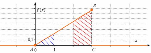
Ну вот, теперь всё наглядно – где бОльшая площадь, там и сконцентрированы более вероятные значения.

Так как функция плотности «собирает под собой» вероятности, то она неотрицательна и её график не может располагаться ниже оси . В общем случае функция разрывна (смотрим, где «жирные» оранжевые точки!).

Теперь разберём весьма любопытный факт: поскольку действительных чисел несчётно много, то вероятность того, что случайная величина примет какое-то конкретное значение стремится к нулю. И поэтому вероятности рассчитывают не для отдельно взятых точек, а для целых промежутков (пусть даже очень малых). Как вы правильно догадываетесь:
(синяя площадь на чертеже) – вероятность того, что случайная величина примет значение из отрезка ;
(красная площадь) – вероятность того, что случайная величина примет значение из отрезка .

По той причине, что отдельно взятые значения можно не принимать во внимание, с помощью этих же интегралов рассчитываются и вероятности по интервалам и полуинтервалам, в частности:

Этим же объяснятся аналогичная «вольность» с функцией .
Возможно, кто-то спросит: а зачем считать интегралы, если есть функция ?

А дело в том, что во многих задачах непрерывная случайная величина ИЗНАЧАЛЬНО задана функцией плотности распределения, которая ТОЖЕ однозначно определяет случайную величину. Но, как вариант, можно сначала найти функцию (с помощью тех же интегралов), после чего использовать «лёгкий способ» бросить курить отыскания вероятностей. Впрочем, об этом чуть позже:

Задача 105
Непрерывная случайная величина задана своей функцией распределения:

Найти значения и функцию . Проверить, что действительно является функцией плотности распределения. Вычислить вероятности . Построить графики .

Тренируемся самостоятельно! Если возникнут затруднения, то внимательно перечитайте вышеизложенный материал. Краткое решение и ответ в конце книги.

Вообще, типовые задачи на непрерывную случайную величину можно разделить на 2 большие группы:

1) когда дана функция , 2) когда дана функция .

В первом случае не составляет особых трудностей отыскать функцию плотности распределения – почти всегда производные не то что простЫ, а примитивны (в чём мы только что убедились). Но вот когда НСВ задана функцией , то нахождение функции распределения – есть более кропотливый процесс:
Задача 106
Непрерывная случайная величина задана функцией плотности распределения:

Найти значение и составить функцию распределения вероятностей . Вычислить .
Построить графики .

Решение: найдём константу . Это классика (в подавляющем большинстве задач вам не предложат готовую функцию плотности). Используем свойство .
В данном случае:

На практике нулевые интегралы можно опускать, а константу сразу выносить за знак интеграла:
(*)
Пользуясь чётностью подынтегральной функции, вычислим интеграл:
и подставим результат в уравнение (*):
, откуда выразим

Таким образом, функция плотности распределения:

Выполним проверку, а именно, вычислим тот же самый интеграл, но уже с известной константой. Для разнообразия я не буду пользоваться чётностью:
, отлично.

Обратите внимание, что только при и только при этом значении предложенная в условии функция является функцией плотности распределения. Ну и тут не лишним будет проконтролировать, что на интервале , т.е. условие неотрицательности действительно выполнено. Доверяй условию, да проверяй Не раз и не два мне встречались функции, которые в принципе не могли быть плотностью, что говорило об опечатках или о невнимательности авторов задач.

Теперь начинается самое интересное. Функции распределения вероятностей – есть интеграл:

Так как состоит из трёх кусков, то решение разобьётся на 3 шага:

1) На промежутке , поэтому:

2) На интервале , и мы прицепляем следующий вагончик:

При подстановке верхнего предела интегрирования можно считать, что вместо «икс» мы подставляем «икс». Если же возник вопрос с пределом нижним, то вспоминаем график синуса либо его нечётность: .

3) И, наконец, на , и детский паровозик отправляется в путь:

Внимание! А вот в этом задании нулевые интегралы пропускать НЕ НАДО. Чтобы показать своё понимание функции распределения К тому же, они могут оказаться вовсе не нулевыми, и тогда придётся иметь дело с интегралами несобственными. И такой пример я обязательно разберу ниже.

Записываем наши достижения под единую скобку:

С высокой вероятностью всё правильно, но, тем не менее, устно возьмём производную: , а также «прозвоним» точки «стыка»:

Правильность решения можно проконтролировать и в ходе построения графика, но, во-первых, он не всегда требуется, а во-вторых, до сего момента можно успеть «наломать дров». Ибо вероятности попадания чаще находят с помощью функции распределения:

– вероятность того, что случайная величина примет значение из промежутка

Второй способ состоит в вычислении интеграла:
что, кстати, не труднее. И проверочка заодно получилась.

Выполним чертежи. График представляет собой косинусоиду, сжатую вдоль ординат в 2 раза. Тот редкий случай, когда функция плотности непрерывна:

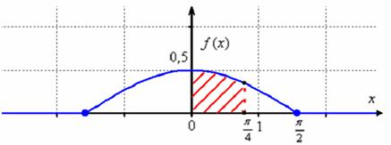
Значение численно равно заштрихованной площади – это я специально нарисовал, чтобы напомнить вероятностный смысл плотности функции распределения. И вся площадь под «дугой» равна единице, то есть, достоверным является тот факт, что случайная величина примет значение из интервала . Заметьте, что значения по условию, невозможны.
Осталось изобразить функцию распределения. График представляет собой синусоиду, сжатую в 2 раза вдоль оси ординат и сдвинутую на вверх:

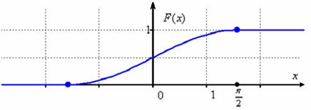
В принципе, тут можно было не заморачиваться преобразованием графиков, а найти несколько опорных точек и догадаться, как выглядит кривая (тригонометрическая таблица в помощь). Но «любительский» подход чреват тем, что график получится принципиально не точным. Так, в нашем примере в точке существует перегиб графика функции , и велик риск неверно отобразить его выпуклость / вогнутость.

Чертежи желательно расположить так, чтобы оси ординат (вертикальные оси) лежали ровненько одна под другой. Это будет хорошим тоном.

И я так чувствую, вам уже не терпится проверить свои силы. Как водится, пример попроще:

Задача 107
Задана плотность распределения вероятностей непрерывной случайной величины :

Требуется:

1) определить коэффициент ;
2) найти функцию распределения ;
3) построить графики ;
4) найти вероятность того, что примет значение из промежутка

и задачка поинтереснее:

Задача 108
Непрерывная случайная величина задана плотностью распределения вероятностей:

Найти значение и построить график плотности распределения. Найти функцию распределения вероятностей и построить её график. Вычислить вероятность .

Дерзайте! Свериться с решением можно внизу книги.

Следует отметить, что все эти задачи реально предлагают студентам-заочникам, и поэтому я не предлагаю вам ничего необычного.

И в заключение параграфа обещанные случаи с несобственными интегралами:

Задача 109
Непрерывная случайная величина задана своей плотностью распределения:

Найти коэффициент и функцию распределения . Построить графики.

Решение: по свойству функции плотности распределения:

В данной задаче состоит из 2 частей, поэтому:

Правый интеграл равен нулю, а вот левый – есть «живой» несобственный интеграл с бесконечным нижним пределом:

Таким образом, наше уравнение превратилось в готовый результат:

и функция плотности:

Функция , как нетрудно понять, отыскивается в 2 шага:

1) На промежутке , следовательно:
– вот такая вот у нас замечательная экспонента. Как птица Феникс.

2) На интервале и:
, что и должно получиться.

Для построения графиков найдём пару опорных точек: и аккуратно прочертим кусочки экспонент с причитающимися дополнениями:

Заметьте, что теоретически случайная величина может принять сколь угодно большое по модулю отрицательное значение, и ось абсцисс является горизонтальной асимптотой для обоих графиков при .

В соответствующей статье сайта я рассмотрел ещё более интересный пример с функцией , где случайная величина теоретически принимает вообще ВСЕ действительные значения. Но это уже несколько повышенный уровень сложности.

2.4.4. Как вычислить математическое ожидание и дисперсию НСВ?

2.4.2. Вероятность попадания в промежуток

| Оглавление |

Полную и свежую версию этой книги в pdf-формате,
а также курсы по другим темам можно найти здесь.

Также вы можете изучить эту тему подробнее – просто, доступно, весело и бесплатно!

С наилучшими пожеланиями, Александр Емелин

Источник

Плотность распределения вероятностей непрерывной случайной величины

Краткая теория

Свойства плотности распределения

Примеры решения задач

Пример 1

Пример 2

Пример 3

Задачи контрольных и самостоятельных работ

Example[edit]

Absolutely continuous univariate distributions[edit]

Formal definition[edit]

Discussion[edit]

Further details[edit]

Link between discrete and continuous distributions[edit]

Families of densities[edit]

Densities associated with multiple variables[edit]

Marginal densities[edit]

Independence[edit]

Corollary[edit]

Example[edit]

Function of random variables and change of variables in the probability density function[edit]

Scalar to scalar[edit]

Vector to vector[edit]

Vector to scalar[edit]

Sums of independent random variables[edit]

Products and quotients of independent random variables[edit]

Example: Quotient distribution[edit]

Example: Quotient of two standard normals[edit]

See also[edit]

References[edit]

Further reading[edit]

External links[edit]

2.4.3. Функция ПЛОТНОСТИ распределения вероятностей