Как найти групповую скорость волны

From Wikipedia, the free encyclopedia

«Wave group» redirects here. Not to be confused with Wave packet.

Frequency dispersion in groups of gravity waves on the surface of deep water. The red square moves with the phase velocity, and the green circles propagate with the group velocity. In this deep-water case, the phase velocity is twice the group velocity. The red square overtakes two green circles when moving from the left to the right of the figure.

New waves seem to emerge at the back of a wave group, grow in amplitude until they are at the center of the group, and vanish at the wave group front.

For surface gravity waves, the water particle velocities are much smaller than the phase velocity, in most cases.

Propagation of a wave packet demonstrating a phase velocity greater than the group velocity without dispersion.

This shows a wave with the group velocity and phase velocity going in different directions.^[1] The group velocity is positive (i.e., the envelope of the wave moves rightward), while the phase velocity is negative (i.e., the peaks and troughs move leftward).

The group velocity of a wave is the velocity with which the overall envelope shape of the wave’s amplitudes—known as the modulation or envelope of the wave—propagates through space.

For example, if a stone is thrown into the middle of a very still pond, a circular pattern of waves with a quiescent center appears in the water, also known as a capillary wave. The expanding ring of waves is the wave group, within which one can discern individual waves that travel faster than the group as a whole. The amplitudes of the individual waves grow as they emerge from the trailing edge of the group and diminish as they approach the leading edge of the group.

History[edit]

The idea of a group velocity distinct from a wave’s phase velocity was first proposed by W.R. Hamilton in 1839, and the first full treatment was by Rayleigh in his «Theory of Sound» in 1877.^[2]

Definition and interpretation[edit]

The envelope of the wave packet. The envelope moves at the group velocity.

The group velocity v_g is defined by the equation:^[3]^[4]^[5]^[6]

${displaystyle v_{rm {g}} equiv {frac {partial omega }{partial k}},}$

where ω is the wave’s angular frequency (usually expressed in radians per second), and k is the angular wavenumber (usually expressed in radians per meter). The phase velocity is: v_p = ω/k.

The function ω(k), which gives ω as a function of k, is known as the dispersion relation.

If ω is directly proportional to k, then the group velocity is exactly equal to the phase velocity. A wave of any shape will travel undistorted at this velocity.
If ω is a linear function of k, but not directly proportional (ω = ak + b), then the group velocity and phase velocity are different. The envelope of a wave packet (see figure on right) will travel at the group velocity, while the individual peaks and troughs within the envelope will move at the phase velocity.
If ω is not a linear function of k, the envelope of a wave packet will become distorted as it travels. Since a wave packet contains a range of different frequencies (and hence different values of k), the group velocity ∂ω/∂k will be different for different values of k. Therefore, the envelope does not move at a single velocity, but its wavenumber components (k) move at different velocities, distorting the envelope. If the wavepacket has a narrow range of frequencies, and ω(k) is approximately linear over that narrow range, the pulse distortion will be small, in relation to the small nonlinearity. See further discussion below. For example, for deep water gravity waves, , and hence v_g = v_p /2. This underlies the Kelvin wake pattern for the bow wave of all ships and swimming objects. Regardless of how fast they are moving, as long as their velocity is constant, on each side the wake forms an angle of 19.47° = arcsin(1/3) with the line of travel.^[7]

Derivation[edit]

One derivation of the formula for group velocity is as follows.^[8]^[9]

Consider a wave packet as a function of position x and time t: α(x,t).

Let A(k) be its Fourier transform at time t = 0,

${displaystyle alpha (x,0)=int _{-infty }^{infty }dk,A(k)e^{ikx}.}$

By the superposition principle, the wavepacket at any time t is

${displaystyle alpha (x,t)=int _{-infty }^{infty }dk,A(k)e^{i(kx-omega t)},}$

where ω is implicitly a function of k.

Assume that the wave packet α is almost monochromatic, so that A(k) is sharply peaked around a central wavenumber k₀.

Then, linearization gives

${displaystyle omega (k)approx omega _{0}+left(k-k_{0}right)omega '_{0}}$

where

${displaystyle omega _{0}=omega (k_{0})}$

and ${displaystyle omega '_{0}=left.{frac {partial omega (k)}{partial k}}right|_{k=k_{0}}}$

(see next section for discussion of this step). Then, after some algebra,

${displaystyle alpha (x,t)=e^{ileft(k_{0}x-omega _{0}tright)}int _{-infty }^{infty }dk,A(k)e^{i(k-k_{0})left(x-omega '_{0}tright)}.}$

There are two factors in this expression. The first factor, ${displaystyle e^{ileft(k_{0}x-omega _{0}tright)}}$ , describes a perfect monochromatic wave with wavevector k₀, with peaks and troughs moving at the phase velocity $omega _{0}/k_{0}$ within the envelope of the wavepacket.

The other factor,

${displaystyle int _{-infty }^{infty }dk,A(k)e^{i(k-k_{0})left(x-omega '_{0}tright)}}$

gives the envelope of the wavepacket. This envelope function depends on position and time only through the combination ${displaystyle (x-omega '_{0}t)}$ .

Therefore, the envelope of the wavepacket travels at velocity

${displaystyle omega '_{0}=left.{frac {domega }{dk}}right|_{k=k_{0}}~,}$

which explains the group velocity formula.

Other expressions[edit]

For light, the refractive index n, vacuum wavelength λ₀, and wavelength in the medium λ, are related by

${displaystyle lambda _{0}={frac {2pi c}{omega }},;;lambda ={frac {2pi }{k}}={frac {2pi v_{rm {p}}}{omega }},;;n={frac {c}{v_{rm {p}}}}={frac {lambda _{0}}{lambda }},}$

with v_p = ω/k the phase velocity.

The group velocity, therefore, can be calculated by any of the following formulas,

${displaystyle {begin{aligned}v_{rm {g}}&={frac {c}{n+omega {frac {partial n}{partial omega }}}}={frac {c}{n-lambda _{0}{frac {partial n}{partial lambda _{0}}}}}\&=v_{rm {p}}left(1+{frac {lambda }{n}}{frac {partial n}{partial lambda }}right)=v_{rm {p}}-lambda {frac {partial v_{rm {p}}}{partial lambda }}=v_{rm {p}}+k{frac {partial v_{rm {p}}}{partial k}}.end{aligned}}}$

Dispersion[edit]

Distortion of wave groups by higher-order dispersion effects, for surface gravity waves on deep water (with v_g = ½v_p).

This shows the superposition of three wave components—with respectively 22, 25 and 29 wavelengths fitting in a periodic horizontal domain of 2 km length. The wave amplitudes of the components are respectively 1, 2 and 1 meter.

Part of the previous derivation is the Taylor series approximation that:

${displaystyle omega (k)approx omega _{0}+(k-k_{0})omega '_{0}(k_{0})}$

If the wavepacket has a relatively large frequency spread, or if the dispersion ω(k) has sharp variations (such as due to a resonance), or if the packet travels over very long distances, this assumption is not valid, and higher-order terms in the Taylor expansion become important.

As a result, the envelope of the wave packet not only moves, but also distorts, in a manner that can be described by the material’s group velocity dispersion. Loosely speaking, different frequency-components of the wavepacket travel at different speeds, with the faster components moving towards the front of the wavepacket and the slower moving towards the back. Eventually, the wave packet gets stretched out. This is an important effect in the propagation of signals through optical fibers and in the design of high-power, short-pulse lasers.

Relation to phase velocity, refractive index and transmission speed[edit]

A superposition of 1D plane waves (blue) each traveling at a different phase velocity (traced by blue dots) results in a Gaussian wave packet (red) that propagates at the group velocity (traced by the red line).

The group velocity of a collection of waves is defined as

${displaystyle v_{g}={frac {partial omega }{partial k}}.}$

When multiple sinusoidal waves are propagating together, the resultant superposition of the waves can result in an «envelope» wave as well as a «carrier» wave that lies inside the envelope. This commonly appears in wireless communication when modulation (a change in amplitude and/or phase) is employed to send data. To gain some intuition for this definition, we consider a superposition of (cosine) waves f(x, t) with their respective angular frequencies and wavevectors.

${displaystyle {begin{aligned}f(x,t)&=cos(k_{1}x-omega _{1}t)+cos(k_{2}x-omega _{2}t)\&=2cos left({frac {(k_{2}-k_{1})x-(omega _{2}-omega _{1})t}{2}}right)cos left({frac {(k_{2}+k_{1})x-(omega _{2}+omega _{1})t}{2}}right)\&=2f_{1}(x,t)f_{2}(x,t).end{aligned}}}$

So, we have a product of two waves: an envelope wave formed by f₁ and a carrier wave formed by f₂ . We call the velocity of the envelope wave the group velocity. We see that the phase velocity of f₁ is

${displaystyle {frac {omega _{2}-omega _{1}}{k_{2}-k_{1}}}.}$

In the continuous differential case, this becomes the definition of the group velocity.

In the context of electromagnetics and optics, the frequency is some function ω(k) of the wave number, so in general, the phase velocity and the group velocity depend on specific medium and frequency. The ratio between the speed of light c and the phase velocity v_p is known as the refractive index, n = c / v_p = ck / ω.

In this way, we can obtain another form for group velocity for electromagnetics. Writing n = n(ω), a quick way to derive this form is to observe

${displaystyle k={frac {1}{c}}omega n(omega )implies dk={frac {1}{c}}left(n(omega )+omega {frac {partial }{partial omega }}n(omega )right)domega .}$

We can then rearrange the above to obtain

${displaystyle v_{g}={frac {partial w}{partial k}}={frac {c}{n+omega {frac {partial n}{partial omega }}}}.}$

From this formula, we see that the group velocity is equal to the phase velocity only when the refractive index is a constant dn / dk = 0. When this occurs, the medium is called non-dispersive, as opposed to dispersive, where various properties of the medium depend on the frequency ω. The relation ω = ω(k) is known as the dispersion relation of the medium.

In three dimensions[edit]

For waves traveling through three dimensions, such as light waves, sound waves, and matter waves, the formulas for phase and group velocity are generalized in a straightforward way:^[10]

where

${displaystyle {vec {nabla }}_{mathbf {k} },omega }$

means the gradient of the angular frequency ω as a function of the wave vector , and is the unit vector in direction k.

If the waves are propagating through an anisotropic (i.e., not rotationally symmetric) medium, for example a crystal, then the phase velocity vector and group velocity vector may point in different directions.

In lossy or gainful media[edit]

The group velocity is often thought of as the velocity at which energy or information is conveyed along a wave. In most cases this is accurate, and the group velocity can be thought of as the signal velocity of the waveform. However, if the wave is travelling through an absorptive or gainful medium, this does not always hold. In these cases the group velocity may not be a well-defined quantity, or may not be a meaningful quantity.

In his text “Wave Propagation in Periodic Structures”,^[11] Brillouin argued that in a dissipative medium the group velocity ceases to have a clear physical meaning. An example concerning the transmission of electromagnetic waves through an atomic gas is given by Loudon.^[12] Another example is mechanical waves in the solar photosphere: The waves are damped (by radiative heat flow from the peaks to the troughs), and related to that, the energy velocity is often substantially lower than the waves’ group velocity.^[13]

Despite this ambiguity, a common way to extend the concept of group velocity to complex media is to consider spatially damped plane wave solutions inside the medium, which are characterized by a complex-valued wavevector. Then, the imaginary part of the wavevector is arbitrarily discarded and the usual formula for group velocity is applied to the real part of wavevector, i.e.,

${displaystyle v_{rm {g}}=left({frac {partial left(operatorname {Re} kright)}{partial omega }}right)^{-1}.}$

Or, equivalently, in terms of the real part of complex refractive index, n = n + iκ, one has^[14]

${displaystyle {frac {c}{v_{rm {g}}}}=n+omega {frac {partial n}{partial omega }}.}$

It can be shown that this generalization of group velocity continues to be related to the apparent speed of the peak of a wavepacket.^[15] The above definition is not universal, however: alternatively one may consider the time damping of standing waves (real k, complex ω), or, allow group velocity to be a complex-valued quantity.^[16]^[17] Different considerations yield distinct velocities, yet all definitions agree for the case of a lossless, gainless medium.

The above generalization of group velocity for complex media can behave strangely, and the example of anomalous dispersion serves as a good illustration.
At the edges of a region of anomalous dispersion, ${displaystyle v_{rm {g}}}$ becomes infinite (surpassing even the speed of light in vacuum), and ${displaystyle v_{rm {g}}}$ may easily become negative
(its sign opposes Rek) inside the band of anomalous dispersion.^[18]^[19]^[20]

Superluminal group velocities[edit]

Since the 1980s, various experiments have verified that it is possible for the group velocity (as defined above) of laser light pulses sent through lossy materials, or gainful materials, to significantly exceed the speed of light in vacuum c. The peaks of wavepackets were also seen to move faster than c.

In all these cases, however, there is no possibility that signals could be carried faster than the speed of light in vacuum, since the high value of v_g does not help to speed up the true motion of the sharp wavefront that would occur at the start of any real signal. Essentially the seemingly superluminal transmission is an artifact of the narrow band approximation used above to define group velocity and happens because of resonance phenomena in the intervening medium. In a wide band analysis it is seen that the apparently paradoxical speed of propagation of the signal envelope is actually the result of local interference of a wider band of frequencies over many cycles, all of which propagate perfectly causally and at phase velocity. The result is akin to the fact that shadows can travel faster than light, even if the light causing them always propagates at light speed; since the phenomenon being measured is only loosely connected with causality, it does not necessarily respect the rules of causal propagation, even if it under normal circumstances does so and leads to a common intuition.^[14]^[18]^[19]^[21]^[22]

References[edit]

Notes[edit]

^ Nemirovsky, Jonathan; Rechtsman, Mikael C; Segev, Mordechai (9 April 2012). «Negative radiation pressure and negative effective refractive index via dielectric birefringence». Optics Express. 20 (8): 8907–8914. Bibcode:2012OExpr..20.8907N. doi:10.1364/OE.20.008907. PMID 22513601.
^ Brillouin, Léon (1960), Wave Propagation and Group Velocity, New York: Academic Press Inc., OCLC 537250
^ Brillouin, Léon (2003) [1946], Wave Propagation in Periodic Structures: Electric Filters and Crystal Lattices, Dover, p. 75, ISBN 978-0-486-49556-9
^ Lighthill, James (2001) [1978], Waves in fluids, Cambridge University Press, p. 242, ISBN 978-0-521-01045-0
^ Lighthill (1965)
^ Hayes (1973)
^ G.B. Whitham (1974). Linear and Nonlinear Waves (John Wiley & Sons Inc., 1974) pp 409–410 Online scan
^
Griffiths, David J. (1995). Introduction to Quantum Mechanics. Prentice Hall. p. 48. ISBN 9780131244054.
^
David K. Ferry (2001). Quantum Mechanics: An Introduction for Device Physicists and Electrical Engineers (2nd ed.). CRC Press. pp. 18–19. Bibcode:2001qmid.book…..F. ISBN 978-0-7503-0725-3.
^ Atmospheric and oceanic fluid dynamics: fundamentals and large-scale circulation, by Geoffrey K. Vallis, p239
^ Brillouin, L. (1946). Wave Propagation in Periodic Structures. New York: McGraw Hill.
^ Loudon, R. (1973). The Quantum Theory of Light. Oxford.
^ Worrall, G. (2012). «On the Effect of Radiative Relaxation on the Flux of Mechanical-Wave Energy in the Solar Atmosphere». Solar Physics. 279 (1): 43–52. Bibcode:2012SoPh..279…43W. doi:10.1007/s11207-012-9982-z. S2CID 119595058.
^ ^a ^b Boyd, R. W.; Gauthier, D. J. (2009). «Controlling the velocity of light pulses» (PDF). Science. 326 (5956): 1074–7. Bibcode:2009Sci…326.1074B. CiteSeerX 10.1.1.630.2223. doi:10.1126/science.1170885. PMID 19965419. S2CID 2370109.
^ Morin, David (2009). «Dispersion» (PDF). people.fas.harvard.edu. Archived (PDF) from the original on 2012-05-21. Retrieved 2019-07-11.
^ Muschietti, L.; Dum, C. T. (1993). «Real group velocity in a medium with dissipation». Physics of Fluids B: Plasma Physics. 5 (5): 1383. Bibcode:1993PhFlB…5.1383M. doi:10.1063/1.860877.
^ Gerasik, Vladimir; Stastna, Marek (2010). «Complex group velocity and energy transport in absorbing media». Physical Review E. 81 (5): 056602. Bibcode:2010PhRvE..81e6602G. doi:10.1103/PhysRevE.81.056602. PMID 20866345.
^ ^a ^b Dolling, Gunnar; Enkrich, Christian; Wegener, Martin; Soukoulis, Costas M.; Linden, Stefan (2006), «Simultaneous Negative Phase and Group Velocity of Light in a Metamaterial», Science, 312 (5775): 892–894, Bibcode:2006Sci…312..892D, doi:10.1126/science.1126021, PMID 16690860, S2CID 29012046
^ ^a ^b Bigelow, Matthew S.; Lepeshkin, Nick N.; Shin, Heedeuk; Boyd, Robert W. (2006), «Propagation of a smooth and discontinuous pulses through materials with very large or very small group velocities», Journal of Physics: Condensed Matter, 18 (11): 3117–3126, Bibcode:2006JPCM…18.3117B, doi:10.1088/0953-8984/18/11/017, S2CID 38556364
^ Withayachumnankul, W.; Fischer, B. M.; Ferguson, B.; Davis, B. R.; Abbott, D. (2010), «A Systemized View of Superluminal Wave Propagation», Proceedings of the IEEE, 98 (10): 1775–1786, doi:10.1109/JPROC.2010.2052910, S2CID 15100571
^ Gehring, George M.; Schweinsberg, Aaron; Barsi, Christopher; Kostinski, Natalie; Boyd, Robert W. (2006), «Observation of a Backward Pulse Propagation Through a Medium with a Negative Group Velocity», Science, 312 (5775): 895–897, Bibcode:2006Sci…312..895G, doi:10.1126/science.1124524, PMID 16690861, S2CID 28800603
^ Schweinsberg, A.; Lepeshkin, N. N.; Bigelow, M.S.; Boyd, R. W.; Jarabo, S. (2005), «Observation of superluminal and slow light propagation in erbium-doped optical fiber» (PDF), Europhysics Letters, 73 (2): 218–224, Bibcode:2006EL…..73..218S, CiteSeerX 10.1.1.205.5564, doi:10.1209/epl/i2005-10371-0, S2CID 250852270

External links[edit]

Greg Egan has an excellent Java applet on his web site that illustrates the apparent difference in group velocity from phase velocity.
Maarten Ambaum has a webpage with movie demonstrating the importance of group velocity to downstream development of weather systems.
Phase vs. Group Velocity – Various Phase- and Group-velocity relations (animation)

Источник

Фазовая и групповая скорость волны, формула Рэлея.

Годжаев гл.2 с.1-3
п.2(весь).

Распространение электромагнитной волны. Фазовая и групповая скорости Фазовая скорость.

Выше мы ознакомились
с некоторыми свойствами электромагнитной
волны. Теперь более подробно рассмотрим
распространение световой волны и
ознакомимся с понятиями фазовой и
групповой скоростей.

Рассмотрим
плоскую монохроматическую световую
волну, распространяющуюся в
положительном направлении оси к
в
однородной среде:

(4.36)

где,
как мы уже отметили,

Можно
легко доказать, что v
является
скоростью перемещения поверхности
равных фаз (волновой поверхности). В
самом деле, уравнение поверхности равных
фаз имеет вид

(4.37)

Дифференцируя
это выражение по t,
найдем
скорость перемещения волновой поверхности
вдоль оси х,
которую
принято называть фазовой скоростью:

(4.38)

Используя
выражение фазы через волновое число k,
можно
получить формулу для определения
фазовой скорости:

Дифференцируя
по t,
получим,

(4.39) Следовательно,монохроматическую
волну можно характеризовать одной
лишь фазовой скоростью

Групповая скорость.

Можно
было бы ограничиться только понятием
фазовой скорости, если бы монохроматические
волны реально существовали. Однако
отдельные атомы излучают в действительности
не бесконечные во времени монохроматические
волны, а своего рода световые импульсы.
Подобный «световой импульс может
быть смоделирован в виде «кусочка»
монохроматической волны длительности
∆t,
как это показано на рис.2.4. Немонохроматичность
световых волн и обусловлена в основном
обрывом монохроматической волны.

Как
увидим в дальнейшем (см. § 4 и 5 этой
главы), конечные импульсы можно представить
в виде совокупности гармонических
колебаний с разными амплитудами,
частотами и фазами. Пусть ∆ω — интервал,
в пределах которого лежат упомянутые
частоты. Ширина интервала ∆ω зависит
от длительности импульса. Можно показать,
что интервал частот обратно пропорционален
длительности импульса, т. е.

Форма импульса
определяется частотами, амплитудами и
фазами его гармонических составляющих.
Если скорости всех этих составляющих
одинаковы, то их фазовые соотношения
не меняются при распространении и,
следовательно, форма импульса также
остается неизменной. В этом случае
скорость перемещения импульса совпадает
со скоростью его гармонических
составляющих. Среда, в которой фазовая
скорость гармонической волны не зависит
от частоты, называется недиспергирующей.
В случае, если скорости

.РИС(4.11)
гармонических
волн зависят от частоты, фазовые
соотношения между ними меняются по мере
их распространения, что приводит к
изменению формы импульса. Отсюда
следует, что скорость перемещения
импульса и фазовая скорость его
гармонических составляющих не
совпадают.
В этом случае распространение импульса
характеризуют с помощью так называемой
групповой скорости. Среда, в которой
фазовая скорость зависит от частоты,
называется диспергирующей.

Введем
групповую скорость для случая простейшей
группы, состоящей из двух гармонических
составляющих одинаковой амплитуды,
мало отличающихся по частоте и
распространяющихся вдоль оси х:

(4.40)

Результирующая
волна будет иметь вид

(4.41)

По
условию,

Учитывая
это, получим

(4.42)

Где

Полученное
выражение (2.24) для сложной волны можно
приближенно считать уравнением
монохроматической волны с частотой
co_1?
волновым числом &i
и медленно меняющейся (модулиро-

ванной) амплитудой

(4.43)

Если
такой модулированный
по амплитуде импульс принимается
спектральным приоо-ром, то он будет
регистрировать две частоты: ω₁и
ω₂.

Модулированная
амплитуда характеризует группу волн.
Поэтому распространение импульса
можно характеризовать скоростью переноса
определенного значения модулированной
амплитуды. Эту скорость называют
групповой скоростью волн. Так как на
опыте удобно регистрировать максимальную
амплитуду, то под групповой скоростью
понимают скорость перемещения максимума
амплитуды волны. Следовательно, групповая
скорость определяется из условия

(4.44)

где
т
—
любое целое число. После дифференцирования
(2.25) по t
получим

(4.45)

В пределе можно перейти
к дифференциалу:

(4.46)

Связь
между
фазовой
и групповой скоростями.
Исходя из (2.26) и (2.22) можно найти связь
между фазовой и групповой скоростями:

(4.47)

Так
как

и
отсюда

то
из (2.27) имеем

(4.48)

Полученное
выражение (2.28) носит название формулы
Рэлея. Им же было впервые введено
понятие групповой скорости.

Соседние файлы в предмете [НЕСОРТИРОВАННОЕ]

Источник

Сергей Сергеевич Соев

Эксперт по предмету «Физика»

Задать вопрос автору статьи

Фазовая скорость

Монохроматическая волна вида:

является бесконечной во времени и пространстве последовательностью «горбов и впадин», которые распространяются по оси $X$. Причем фазовая скорость перемещения максимумов и минимумов равна:

Скорость $v$ — означает скорость перемещения фазы. Используя такую волну нельзя передать сигнал, так как все «горбы» эквивалентны. Для того чтобы передавать сигнал следует сделать на волне «метку» (например сделать некоторый обрыв на конечное время $triangle t$). Но при этом волна уже не будет соответствовать уравнению (1).

Сигнал можно передать, используя импульс света. По теореме Фурье его можно разложить в ряд с частотами в интервале $triangle omega .$ Совокупность волн, которые различаются друг с другом, частотой в пределах малого интервала $triangle omega $ называют волновым пакетом (группой волн). Аналитически волновой пакет можно представить как:

где индекс $omega $ у величин $A, k, alpha $ показывает, что они относятся к разным частотам. В пределах пакета плоские волны усиливают друг друга, вне пакета происходит взаимное гашение волн. Для того чтобы сумму волн, которую описывает выражение (3), можно было считать пакетом, должно выполняться условие: $triangle omega ll {omega }_0.$

Групповая скорость

При отсутствии дисперсии все плоские волны в пакете распространяются с фазовой скоростью $v$. При таких условиях скорость распространения группы волн совпадает с фазовой скоростью, форма пакета постоянна. В веществе при наличии дисперсии пакет со временем ширина пакета увеличивается. При малой дисперсии, скорость перемещения центра пакета (точка, в которой максимальна величина $E$) называют групповой скоростью $(u).$ Групповая скорость характеризует импульс, и соответствует скорости распространения энергии поля этого импульса или скорость перемещения амплитуды.

При наличии дисперсии групповая и фазовая скорость различны:

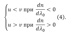
Рисунок 1.

«Фазовая и групповая скорости и их соотношение, формула Рэлея» 👇

Если пакет представлен двумя составляющими, то групповую скорость можно найти как:

Групповая скорость пакета волн, который задан уравнением (3) может быть определена как:

если в разложении функции $k_{omega }=k_0+{left(frac{dk}{domega }right)}_0left(omega -{omega }_0right)+dots left(7right)$ пренебречь членами высоких порядков. В выражении ${left(frac{dk}{domega }right)}_0$- производная в точке ${omega }_0$. В формуле (6) индекс $0$ опущен, так как не требуется. В таком приближении форма пакета волны постоянна во времени. Если в разложении (7) учесть следующие члены, то пакет волны будет расплываться.

Выражение для групповой скорости (6) можно записать в виде:

Связь групповой и фазовой скоростей (формула Рэлея)

Выражение для групповой скорости можно записать в виде:

Формула (9) называется формулой Рэлея. В том случае, если $frac{dv}{dlambda } >0$ имеют дело с нормальной дисперсией, и $uv$. Выражение (9) можно представить как:

Выражение (10) показывает зависимость групповой скорости от характеристик вещества.

При введении понятия групповой скорости используют случай, когда дисперсия не велика. В противном случае пакет волн быстро деформируется и само понятие групповой скорости не имеет смысла. К примеру, около полосы поглощения среды, в области существенного изменения фазовой скорости в зависимости от частоты формула (9) может дать величину $u$ больше, чем скорость света в вакууме, или отрицательное значение. То есть в такой области формула Рэлея не применима.

Пример 1

Задание: Представьте групповую скорость в виде функции от показателя преломления и длины волны. Чему равна групповая скорость волн в воде, если ${lambda }_1$=656,3 нм. Считайте, что при $t=20{rm^circ!C}$ показатель преломления для этой длины воны $n_1=1,3311$, для ${lambda }_2=643,8$ нм $n_{12}=1,3314.$

Решение:

За основу решения задачи примем определение групповой скорости:

[u=frac{domega }{dk}left(1.1right).]

Зная, что круговая частота связана с длинной волны соотношением:

[omega =frac{2pi с}{nlambda }left(1.2right).]

Волновой вектор можно записать как:

[k=frac{2pi }{lambda }left(1.3right).]

Подставим выражения (1.2) и (1.3) в (1.1), получим:

[u=frac{dleft(frac{2pi с}{nlambda }right)}{dleft(frac{2pi }{lambda }right)}=cfrac{(ndlambda +lambda dn)/n^2{lambda }^2}{dlambda /{lambda }^2}=frac{c}{n}left(1+frac{lambda }{n}frac{dn}{dlambda }right)left(1.4right).]

Подставим данные из условий задачи, проведем вычисления:

[u=frac{3cdot {10}^8}{1,3311}left(1+frac{656,3}{1,3311}frac{0,0003}{12,5}right)=2,28cdot {10}^8left(frac{м}{с}right).]

Ответ: $uleft(n,lambda right)=frac{c}{n}left(1+frac{lambda }{n}frac{dn}{dlambda }right)=2,28cdot {10}^8frac{м}{с}.$

Задание: Найдите выражение групповой скорости ($u$), если фазовая скорость ($v$) представлена выражением: $v=a{lambda }^q,$ где $a=const, q

Решение:

В качестве основы для решения задачи используем формулу Рэлея, определяющую групповую скорость вида:

Используя уравнение изменения фазовой скорости, заданное в условиях задачи найдем $frac{dv}{dlambda }$, имеем:

Подставим (2.2) в формулу Рэлея, получим:

Ответ: $u=v(1-q)$.

Находи статьи и создавай свой список литературы по ГОСТу

Поиск по теме

Источник

History[edit]

Definition and interpretation[edit]

Derivation[edit]

Other expressions[edit]

Dispersion[edit]

Relation to phase velocity, refractive index and transmission speed[edit]

In three dimensions[edit]

In lossy or gainful media[edit]

Superluminal group velocities[edit]

See also[edit]

References[edit]

Notes[edit]

Further reading[edit]

External links[edit]

Фазовая и групповая скорость волны, формула Рэлея.

Распространение электромагнитной волны. Фазовая и групповая скорости Фазовая скорость.

Групповая скорость.

Фазовая скорость

Групповая скорость

Связь групповой и фазовой скоростей (формула Рэлея)