Интерполяционный многочлен Ньютона
ищется в следующем виде:
N(x)
= a0
+ a1(x
– x0)
+ a2(x
– x0)(x
– x1)
+…+ an(x
– x0)(x
– x1)
…(x –
xn–1).
(5.17)
Как и в случае (5.8), для получения рабочей
формулы Ньютона необходимо определить
значения коэффициентов ai.
В отличие от технологии расчета (5.9) для
построения интерполяционного многочлена
Ньютона вводится рабочий аппарат в виде
так называемых конечных разностей
для системы равноотстоящих
интерполяционных узлов и в виде разностных
отношений (разделенные разности)
для произвольной системы узлов.
Пусть заданны равноотстоящие узлы xk
= x0 + kh,
h = xi+1
– xi
= const > 0. Значения
f(x)
в них обозначим f(xk)
= fk
= yk,
k =
.
Конечными разностями первого порядка
принято называть величины
f(xi)
= fi
= fi+1
– fi;
i =
![]()
.
Конечные разности второго порядка
определяются равенствами
![]()
;
i =
.
Конечные разности (k
+ 1)-го порядка определяются через
разности k-го порядка:
![]()
;
i =
;
k =
![]()
.
(5.18)
Конечные разности, как правило, вычисляются
по схеме, представленной в табл. 5.1.
Каждая последующая конечная разность
получается путем вычитания в предыдущей
колонке верхней строки из нижней строки.
Последняя колонка kfi
будет равна нулю. Заметим, что конечные
разности можно выразить непосредственно
через значения функций.
Так, для i-го узла
рабочая формула имеет вид
kfi
=
![]()
;
i =
;
k = 1, 2, … . (5.19)
Таблица 5.1
|
i |
fi |
fi |
2fi |
3fi |
… |
|
0 |
f0 |
||||
|
f0 |
|||||
|
1 |
f1 |
2f0 |
|||
|
f1 |
3f0 |
||||
|
2 |
f2 |
2f1 |
|||
|
f2 |
3f1 |
||||
|
3 |
f3 |
2f2 |
|||
|
f3 |
3f2 |
||||
|
4 |
f4 |
2f3 |
|||
|
… |
… |
… |
… |
… |
… |
Разностными отношениями (разделенными
разностями) первого порядка называются
величины
f(x0,
x1) =
![]()
f(x1,
x2) =
![]()
;
… ,
где xi
– произвольные узлы с соблюдением
приоритетности по величине.
По этим соотношениям составляются
разностные отношения второго порядка:
f(x0,
x1, x2)
=
![]()
;
f(x1,
x2, x3)
=![]()
;
… .
Разделенные разности порядка (k
+ 1), k = 1, 2, …,
определяются при помощи разделенных
разностей предыдущего порядка k
по формуле
f(x0,
x1, …, xk+1)
=
![]()
.
(5.20)
Разностные отношения вычисляются
по схеме, представленной в табл. 5.2.
Таблица 5.2
|
i |
xi |
fi |
f(xi, |
f(xi, |
… |
|
0 |
x0 |
f0 |
|||
|
f(x0, |
|||||
|
1 |
x1 |
f1 |
f(x0, |
||
|
f(x1, |
|||||
|
2 |
x2 |
f2 |
f(x1, |
||
|
f(x2, |
|||||
|
3 |
x3 |
f3 |
f(x2, |
||
|
… |
… |
… |
… |
… |
… |
Для равноотстоящих узлов xk
= x0 + kh
(k =
)
имеет место соотношение между разделенными
и конечными разностями:
f(x0,
x1, …, xk)
=
![]()
k = 0, 1, 2, … . (5.21)
Конечная разность и разделенная разность
порядка n от многочлена
степени (n) равны
постоянной величине и, следовательно,
они для более высокого порядка равны
нулю.
Интерполяционный многочлен Ньютона
для системы равноотстоящих узлов.
В случае равностоящих узлов имеется
много различных формул, построение
которых зависит от расположения точки
интерполирования хТ по
отношению к узлам интерполирования.
Пусть функция f(x)
задана таблицей значений fk
= f(xk)
= yk
в узлах xk
= x0 + kh
(k =
),
h = xk+1
– xk
= const.
На основании условий (5.3) и аппарата
конечных разностей для определения
коэффициентов для искомого многочлена
(5.17) получена формула

,
k =
;
при условии, что 0
= 1; 0! = 1. (5.22)
Подставив (5.22) в (5.17), получим формулу
Ньютона для интерполирования в начале
таблицы:

(5.23)
При этом конечные разности определяются
или по схеме (см. табл. 5.1) или по формуле
для произвольного узла (5.19).
Для практического удобства формула
(5.23) часто записывают в другом виде.
Вводится новая переменная t
= (x – x0)/h.
Тогда
x = x0
+ kh;
![]()
;
![]()
,
…,
![]()
и (5.23) примет вид
N(x0
+ th) = y0
+ t![]()
.
(5.24)
Выражение (5.24) может аппроксимировать
y = f(x)
на всем отрезке [x0,
xn].
Однако с точки зрения повышения точности
расчетов и уменьшения числа членов в
(5.24) рекомендуется ограничиться случаем
t < 1, т. е.
использовать формулу (5.24) для интервала
x0
x x1.
Для других значений аргумента, например
для x1
x x2,
вместо x0 лучше
взять значение x1.
Тогда (5.24) можно записать в виде
N(xi
+ th) = yi
+
![]()
;
i = 0, 1, … . (5.25)
Выражение (5.25) называется первым
интерполяционным многочленом
Ньютона для интерполирования
вперед. Он используется для
вычисления значений функций в точках
левой половины рассматриваемого отрезка.
Это объясняется тем, что разности kyi
вычисляются через значение функции yi,
yi+1,
…, yi+k,
причем i + k
n. Поэтому при больших
значениях i нельзя
вычислить значения разностей высших
порядков (k
n – i).
Например, при i =
n – 3 в (5.25) можно
учесть только y,
2y,
3y.
Для правой половины отрезка разности
рекомендуется вычислять справа
налево. В этом случае t
= (x – xn)
/ h, т. е. t
< 0 и (5.25) можно получить в виде
N(xn
+ th) = yn
+
![]()
.
(5.26)
Полученная формула называется вторым
интерполяционным многочленом Ньютона
для интерполирования назад.
Для интерполирования в середине отрезка
можно использовать интерпретации
многочлена Ньютона – это многочлены
Стирлинга, Гаусса, Бесселя.
Погрешность метода Ньютона:
![]()
,
при t
=![]()
;
– принадлежит
отрезку.
Пример 5.1. Вычислить значение
функции y = f(x),
заданной таблицей в точках x
= 0,1 и x = 0,9.
Строим табл. 5.1 для конечных разностей:
-
x
y =
f(x)у
2у
3у
4у
5у
0
1,2715
1,1937
0,2
2,4652
–0,0146
1,1791
0,0007
0,4
3,6443
–0,0139
–0,0001
1,1652
0,0006
0,0000
0,6
4,8095
–0,0133
–0,0001
1,1919
0,0005
0,8
5,9614
–0,0128
1,1391
1
7,1005
Используя для расчета верхние значения
конечных разностей, получим при x
= 0,1 значение t =
(x – x0)/h
= (0,1 – 0) / 0,2 = 0,5. По формуле (5.24):
f(0,1)
![]()
N(0,1) = 1,2715 + 0,5
1,1937 +
![]()
+
![]()
.
По формуле линейной интерполяции f(0,1)
1,8684;
= {0,0018}.
Значение функции в точке x
= 0,9 вычислим по формуле (5.26). В данном
случае t = (x
– xn)
/ h = (0,9 – 1) / 0,2 =
–0,5. Используя нижние значения конечных
разностей, получим
f(0,9)
N(0,9) = 7,1005 – 0,5
1,1391 –
–
![]()
–![]()
.
Если считать по (5.24) f(0,9)
= 6,532522641.
Линейная интерполяция f(0,9)
= 6,53095; = {0,00155}.
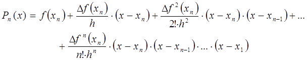
Интерполяционный многочлен Ньютона
для системы произвольно расположенных
узлов. Данный
многочлен строится с помощью аппарата
разделенных разностей (табл. 5.2) в виде
(5.17) на основании имеющего места
соотношения (5.21):
Nn(x)
= f(x0)
+ (x –
x0)
f(x0,
x1)
+ (x –
x0)(x
– x1)
f(x0,
x1,
x2)
+…+
+ (x –
x0)(x
– x1)
… (x –
xn–1)
f(x0,
x1,…,
xn),
(5.27)
где Nn(xk)
= f(xk),
k = 0, 1,
2, …, n.
Остаточный член
Rn(x)
= f(x)
– Nn(x)
= f(x,
x0, x1,
…, xn)(x
– x0)(x
– x1) … (x
– xn).
При n = 1 – это
линейная интерполяция, при n
= 2 – квадратичная.
Замечания:
1. Разные способы построения многочленов
Лагранжа и Ньютона дают тождественные
рабочие формулы при заданной таблице
f(x).
Это следует из единственности
интерполяционного многочлена заданной
степени на упорядоченной системе узлов.
2. Повышение точности интерполирования
предположительно проводить за счет
увеличения числа узлов n
и соответственно степени полинома
Pn(x).
Однако при таком подходе увеличивается
погрешность из-за роста | f
(n)(x)
| и, кроме того, увеличивается вычислительная
погрешность.
Эти соображения приводят к другому
способу приближения функций с помощью
сплайнов (рассмотрено в подразд. 5.5).
3. Повышение точности интерполирования
осуществляется и посредством специального
расположения узлов интерполяции на
рассматриваемом отрезке [a,
b] области определения
функции f(x).
Известно, что если сконцентрировать
узлы xi
вблизи одного конца отрезка [a,
b], то погрешность
Rn(x)
при длине отрезка l =
b – a
> 1 будет велика в точках xi
близких к другому концу. Поэтому всегда
возникает задача о наиболее рациональном
выборе xi
(при заданном числе узлов n).
Эта задача была решена Чебышевым, т. е.
оптимальный выбор узлов нужно производить
по формуле
xi
=
![]()
,
где
![]()
(i = 0, 1, 2, …, n)
нули полинома Чебышева Tn+1(x).
Пример 5.2. Найти значение y
= f(x)
при x = 0,4, заданной
таблично:
|
i |
0 |
1 |
2 |
3 |
|
xi |
0 |
0,1 |
0,3 |
0,5 |
|
yi |
–0,5 |
0 |
0,2 |
1 |
Соседние файлы в предмете [НЕСОРТИРОВАННОЕ]
- #
- #
- #
- #
- #
- #
- #
- #
- #
- #
- #
Выборка экспериментальных данных представляет собой массив данных, который характеризует процесс изменения измеряемого сигнала в течение заданного времени (либо относительно другой переменной). Для выполнения теоретического анализа измеряемого сигнала необходимо найти аппроксимирующую функцию, которая свяжет дискретный набор экспериментальных данных с непрерывной функцией — интерполяционным полиномом n-степени. Данный интерполяционный полином n-степени может быть записан, например, в форме Ньютона (один из способов представления).
Интерполяционный многочлен в форме Ньютона – это математическая функция позволяющая записать полином n-степени, который будет соединять все заданные точки из набора значений, полученных опытным путём или методом случайной выборки с постоянным временным шагом измерений.
1. Интерполяционная формула Ньютона для неравноотстоящих значений аргумента
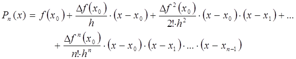
В общем виде интерполяционный многочлен в форме Ньютона записывается в следующем виде:
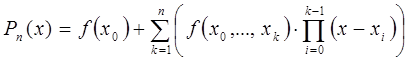
где n – вещественное число, которое указывает степень полинома;
![]() – переменная, которая представляет собой разделенную разность k-го порядка, которая вычисляется по следующей формуле:
– переменная, которая представляет собой разделенную разность k-го порядка, которая вычисляется по следующей формуле:
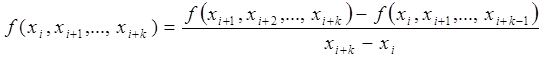
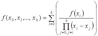
Разделённая разность является симметричной функцией своих аргументов, то есть при любой их перестановке её значение не меняется. Следует отметить, что для разделённой разности k-го порядка справедлива следующая формула:
В качестве примера, рассмотрим построение полинома в форме Ньютона по представленной выборке данных, которая состоит из трех заданных точек ![]() . Интерполяционный многочлен в форме Ньютона, который проходит через три заданных точки, будет записываться в следующем виде:
. Интерполяционный многочлен в форме Ньютона, который проходит через три заданных точки, будет записываться в следующем виде:
![]()
- Разделенная разность 1-го порядка определяется следующим выражением
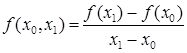
Следует отметить, что данное выражение может быть переписано в другом виде:
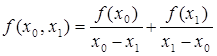
- Разделенная разность 2-го порядка определяется следующим выражением
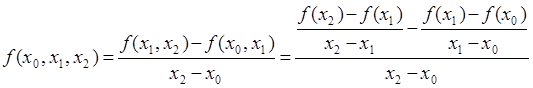
Следует отметить, что данное выражение может быть переписано в другом виде:

Форма Ньютона является удобной формой представления интерполяционного полинома n-степени, так как при добавлении дополнительного узла все вычисленные ранее слагаемые остаются без изменения, а к выражению добавляется только одно новое слагаемое. Следует отметить, что интерполяционный полином в форме Ньютона только по форме отличается от интерполяционного полинома в форме Лагранжа, представляя собой на заданной сетке один и тот же интерполяционный полином.
Следует отметить, что полином в форме Ньютона может быть представлен в более компактном виде (по схеме Горнера), которая получается путем последовательного вынесения за скобки множителей ![]()
![]()
2. Интерполяционная формула Ньютона для равноотстоящих значений аргумента
В случае если значения функции заданы для равноотстоящих значений аргумента, которые имеют постоянный шаг измерений ![]() , то используют другую форму записи интерполяционного многочлена по формуле Ньютона.
, то используют другую форму записи интерполяционного многочлена по формуле Ньютона.
- Для интерполирования функции в конце рассматриваемого интервала (интерполирование назад и экстраполирование вперед) используют интерполяционный полином в форме Ньютона в следующей записи:
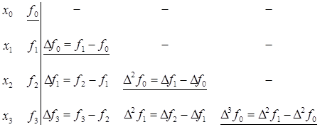
где конечные разности k-порядка определяются по следующему выражению
![]()
Получаемые конечные разности удобно представлять в табличной форме записи, в виде горизонтальной таблице конечных разностей. В этой формуле из таблицы конечных разностей используются ![]() верхней диагонали.
верхней диагонали.
- Для интерполирования функции в начале рассматриваемого интервала (интерполирование вперед и экстраполирование назад) используют интерполяционный полином в форме Ньютона в следующей записи:
где конечные разности k-порядка определяются по следующему выражению
![]()
Получаемые конечные разности удобно представлять в табличной форме записи, в виде горизонтальной таблице конечных разностей. В формуле из таблицы конечных разностей используются ![]() нижней диагонали.
нижней диагонали.

3. Погрешность интерполяционного полинома в форме Ньютона
Рассмотрим функцию f(x), которая непрерывна и дифференцируема на рассматриваемом отрезке [a, b]. Интерполяционный полином P(x) в форме Ньютона принимает в точках ![]() заданные значения функции
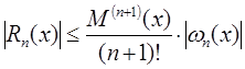
заданные значения функции ![]() . В остальных точках интерполяционный полином P(x) отличается от значения функции f(x) на величину остаточного члена, который определяет абсолютную погрешность интерполяционной формулы Ньютона:
. В остальных точках интерполяционный полином P(x) отличается от значения функции f(x) на величину остаточного члена, который определяет абсолютную погрешность интерполяционной формулы Ньютона:
![]()
Абсолютную погрешность интерполяционной формулы Ньютона определяют следующим образом:
Переменная ![]() представляет собой верхнюю границу значения модуля (n +1)-й производной функции f(x) на заданном интервале [a, b]
представляет собой верхнюю границу значения модуля (n +1)-й производной функции f(x) на заданном интервале [a, b]
![]()
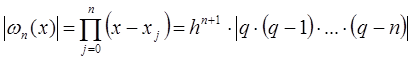
В случае равноотстоящих узлов ![]() абсолютная погрешность интерполяционной формулы Ньютона определяют следующим образом:
абсолютная погрешность интерполяционной формулы Ньютона определяют следующим образом:
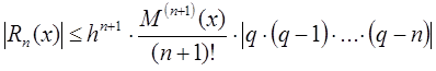
Выражение записано с учетом следующей формулы:
Выбор узлов интерполяции
С помощью корректного выбора узлов можно минимизировать значение ![]() в оценке погрешности, тем самым повысить точность интерполяции. Данная задача может быть решена с помощью многочлена Чебышева:
в оценке погрешности, тем самым повысить точность интерполяции. Данная задача может быть решена с помощью многочлена Чебышева:
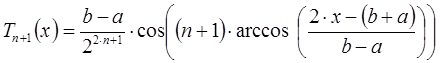
В качестве узлов следует взять корни этого многочлена, то есть точки:
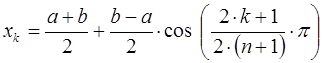
4. Методика вычисления полинома в форме Ньютона (прямой способ)
Алгоритм вычисления полинома в форме Ньютона позволяет разделить задачи определения коэффициентов и вычисления значений полинома при различных значениях аргумента:
1. В качестве исходных данных задается выборка из n-точек, которая включает в себя значения функции и значения аргумента функции.
2. Выполняется вычисление разделенных разностей n-порядка, которые будет использоваться для построения полинома в форме Ньютона.
3. Выполняется вычисление полинома n-степени в форме Ньютона по следующей формуле:
Алгоритм вычисления полинома в форме Ньютона ![]() представлен на рисунке 1.
представлен на рисунке 1.
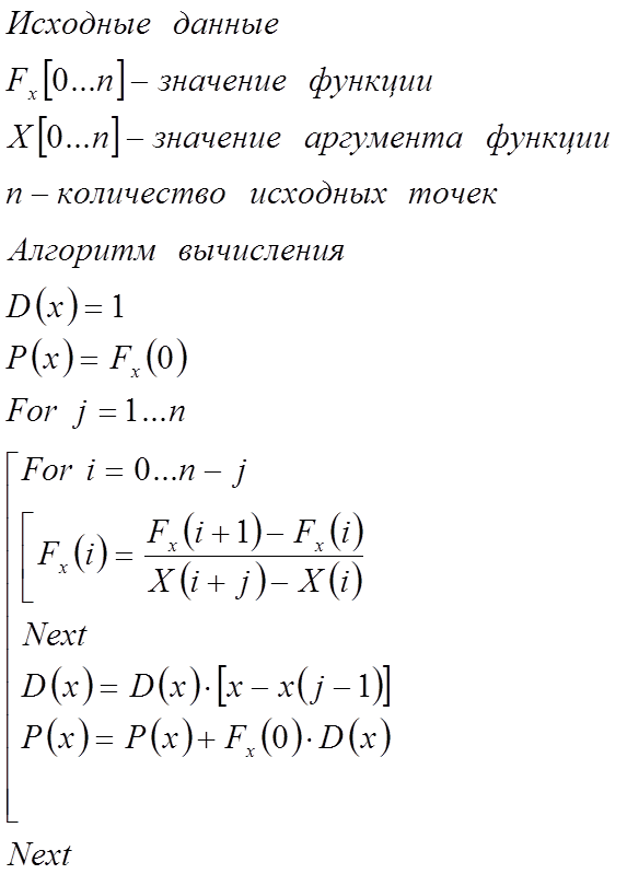
Рис.1. Методика вычисления полинома в форме Ньютона
Следует отметить, что разделённые разности k-го порядка в соответствии с представленной методикой перезаписывается в вектор столбец функции ![]() , а результирующая разделенная разность всегда находится в первой ячейке функций
, а результирующая разделенная разность всегда находится в первой ячейке функций ![]() . Рассмотрим, каким образом будет изменяться вектор столбец функции
. Рассмотрим, каким образом будет изменяться вектор столбец функции ![]() при выполнении расчета по представленной методике.
при выполнении расчета по представленной методике.
В качестве примера рассмотрим следующую практическую задачу. В рамках задачи известен набор шести значений, которые получены методом случайной выборки для различных моментов времени. Следует отметить, что данная выборка значений описывает функция ![]() на интервале [0, 10]. Необходимо построить многочлен в форме Ньютона для представленного набора значений. С помощью интерполяционной формулы вычислить приближенное значение функции в точке
на интервале [0, 10]. Необходимо построить многочлен в форме Ньютона для представленного набора значений. С помощью интерполяционной формулы вычислить приближенное значение функции в точке ![]() , а также определить оценку погрешности результата вычислений.
, а также определить оценку погрешности результата вычислений.
Многочлен в форме Ньютона, который строится на основании шести значений, представляет собой полином 5 степени. Результат построения полинома в форме Ньютона показан в графическом виде.
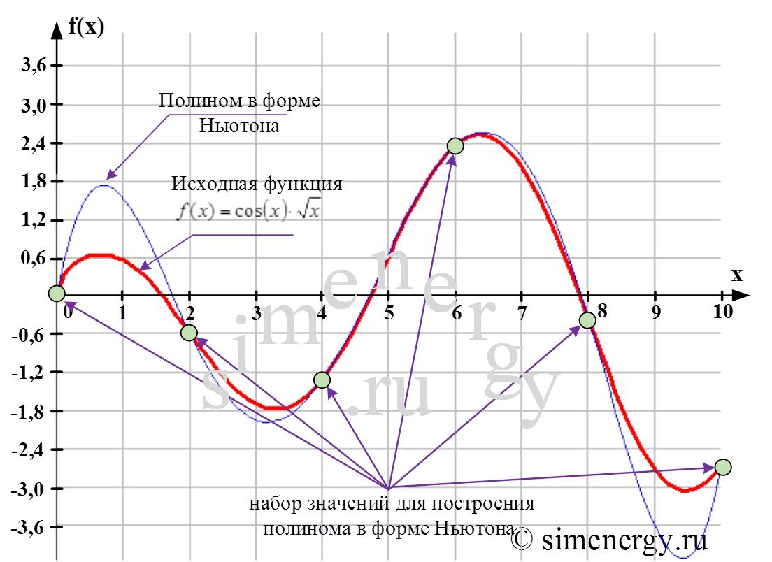
Рис.2. Исходная функция и полином в форме Ньютона, построенный по шести заданным точкам
С помощью найденного полинома можно определить значение функции в любой точке заданного интервала. Определение промежуточных значений величины по имеющемуся дискретному набору известных значений называется «интерполяцией». В соответствии с условиями задачи полином в форме Ньютона в точке x=9,5 принимает следующее значение: L(9,5)= – 4,121. Из графика видно, что полученное значение не совпадает cо значением функции f(x) на величину абсолютной погрешности интерполяционной формулы Ньютона.
Интерполяционный полином в форме Ньютона часто оказывается удобным для проведения различных теоретических исследований в области вычислительной математики. Так, например, полином в форме Ньютона используются для интерполяции, а также для численного интегрирования таблично-заданной функцией.
In the mathematical field of numerical analysis, a Newton polynomial, named after its inventor Isaac Newton,[1] is an interpolation polynomial for a given set of data points. The Newton polynomial is sometimes called Newton’s divided differences interpolation polynomial because the coefficients of the polynomial are calculated using Newton’s divided differences method.
Definition[edit]
Given a set of k + 1 data points

where no two xj are the same, the Newton interpolation polynomial is a linear combination of Newton basis polynomials

with the Newton basis polynomials defined as

for j > 0 and  .
.
The coefficients are defined as
![a_{j}:=[y_{0},ldots ,y_{j}]](https://wikimedia.org/api/rest_v1/media/math/render/svg/f40744c93b8380df3b93026cedb3e03e51e3dd2e)
where
![[y_{0},ldots ,y_{j}]](https://wikimedia.org/api/rest_v1/media/math/render/svg/e845258d4c5470e5c7fdfdaab88ea5e9734aaf16)
is the notation for divided differences.
Thus the Newton polynomial can be written as
![N(x)=[y_{0}]+[y_{0},y_{1}](x-x_{0})+cdots +[y_{0},ldots ,y_{k}](x-x_{0})(x-x_{1})cdots (x-x_{{k-1}}).](https://wikimedia.org/api/rest_v1/media/math/render/svg/b68037ee2fd3c52e2f564605fcd6308048dee2f1)
Newton forward divided difference formula[edit]
The Newton polynomial can be expressed in a simplified form when

are arranged consecutively with equal spacing.
Introducing the notation
 for each
and  ,
,
the difference  can be written as
  .
.
So the Newton polynomial becomes
![{displaystyle {begin{aligned}N(x)&=[y_{0}]+[y_{0},y_{1}]sh+cdots +[y_{0},ldots ,y_{k}]s(s-1)cdots (s-k+1){h}^{k}\&=sum _{i=0}^{k}s(s-1)cdots (s-i+1){h}^{i}[y_{0},ldots ,y_{i}]\&=sum _{i=0}^{k}{s choose i}i!{h}^{i}[y_{0},ldots ,y_{i}].end{aligned}}}](https://wikimedia.org/api/rest_v1/media/math/render/svg/acde564918807b08c1c38188d11e9047abee1176)
This is called the Newton forward divided difference formula.[citation needed]
Newton backward divided difference formula[edit]
If the nodes are reordered as  , the Newton polynomial becomes
![{displaystyle N(x)=[y_{k}]+[{y}_{k},{y}_{k-1}](x-{x}_{k})+cdots +[{y}_{k},ldots ,{y}_{0}](x-{x}_{k})(x-{x}_{k-1})cdots (x-{x}_{1}).}](https://wikimedia.org/api/rest_v1/media/math/render/svg/0f765e4be03523cff51f10707516961d29d30116)
If  are equally spaced with
  and
and  for i = 0, 1, …, k, then,
![{displaystyle {begin{aligned}N(x)&=[{y}_{k}]+[{y}_{k},{y}_{k-1}]sh+cdots +[{y}_{k},ldots ,{y}_{0}]s(s+1)cdots (s+k-1){h}^{k}\&=sum _{i=0}^{k}{(-1)}^{i}{-s choose i}i!{h}^{i}[{y}_{k},ldots ,{y}_{k-i}].end{aligned}}}](https://wikimedia.org/api/rest_v1/media/math/render/svg/833c298afa842a34145ce3631ae774b5712e2675)
is called the Newton backward divided difference formula.[citation needed]
Significance[edit]
Newton’s formula is of interest because it is the straightforward and natural differences-version of Taylor’s polynomial. Taylor’s polynomial tells where a function will go, based on its y value, and its derivatives (its rate of change, and the rate of change of its rate of change, etc.) at one particular x value. Newton’s formula is Taylor’s polynomial based on finite differences instead of instantaneous rates of change.
Addition of new points[edit]
As with other difference formulas, the degree of a Newton interpolating polynomial can be increased by adding more terms and points without discarding existing ones. Newton’s form has the simplicity that the new points are always added at one end: Newton’s forward formula can add new points to the right, and Newton’s backward formula can add new points to the left.
The accuracy of polynomial interpolation depends on how close the interpolated point is to the middle of the x values of the set of points used. Obviously, as new points are added at one end, that middle becomes farther and farther from the first data point. Therefore, if it isn’t known how many points will be needed for the desired accuracy, the middle of the x-values might be far from where the interpolation is done.
Gauss, Stirling, and Bessel all developed formulae to remedy that problem.[2]
Gauss’s formula alternately adds new points at the left and right ends, thereby keeping the set of points centered near the same place (near the evaluated point). When so doing, it uses terms from Newton’s formula, with data points and x values renamed in keeping with one’s choice of what data point is designated as the x0 data point.
Stirling’s formula remains centered about a particular data point, for use when the evaluated point is nearer to a data point than to a middle of two data points.
Bessel’s formula remains centered about a particular middle between two data points, for use when the evaluated point is nearer to a middle than to a data point.
Bessel and Stirling achieve that by sometimes using the average of two differences, and sometimes using the average of two products of binomials in x, where Newton’s or Gauss’s would use just one difference or product. Stirling’s uses an average difference in odd-degree terms (whose difference uses an even number of data points); Bessel’s uses an average difference in even-degree terms (whose difference uses an odd number of data points).
Strengths and weaknesses of various formulae[edit]
For any given finite set of data points, there is only one polynomial of least possible degree that passes through all of them. Thus, it is appropriate to speak of the «Newton form», or Lagrange form, etc., of the interpolation polynomial. However, different methods of computing this polynomial can have differing computational efficiency. There are several similar methods, such as those of Gauss, Bessel and Stirling. They can be derived from Newton’s by renaming the x-values of the data points, but in practice they are important.
Bessel vs. Stirling[edit]
The choice between Bessel and Stirling depends on whether the interpolated point is closer to a data point, or closer to a middle between two data points.
A polynomial interpolation’s error approaches zero, as the interpolation point approaches a data-point. Therefore, Stirling’s formula brings its accuracy improvement where it is least needed and Bessel brings its accuracy improvement where it is most needed.
So, Bessel’s formula could be said to be the most consistently accurate difference formula, and, in general, the most consistently accurate of the familiar polynomial interpolation formulas.
Divided-Difference Methods vs. Lagrange[edit]
Lagrange is sometimes said to require less work, and is sometimes recommended for problems in which it is known, in advance, from previous experience, how many terms are needed for sufficient accuracy.
The divided difference methods have the advantage that more data points can be added, for improved accuracy. The terms based on the previous data points can continue to be used. With the ordinary Lagrange formula, to do the problem with more data points would require re-doing the whole problem.
There is a «barycentric» version of Lagrange that avoids the need to re-do the entire calculation when adding a new data point. But it requires that the values of each term be recorded.
But the ability, of Gauss, Bessel and Stirling, to keep the data points centered close to the interpolated point gives them an advantage over Lagrange, when it isn’t known, in advance, how many data points will be needed.
Additionally, suppose that one wants to find out if, for some particular type of problem, linear interpolation is sufficiently accurate. That can be determined by evaluating the quadratic term of a divided difference formula. If the quadratic term is negligible—meaning that the linear term is sufficiently accurate without adding the quadratic term—then linear interpolation is sufficiently accurate. If the problem is sufficiently important, or if the quadratic term is nearly big enough to matter, then one might want to determine whether the sum of the quadratic and cubic terms is large enough to matter in the problem.
Of course, only a divided-difference method can be used for such a determination.
For that purpose, the divided-difference formula and/or its x0 point should be chosen so that the formula will use, for its linear term, the two data points between which the linear interpolation of interest would be done.
The divided difference formulas are more versatile, useful in more kinds of problems.
The Lagrange formula is at its best when all the interpolation will be done at one x value, with only the data points’ y values varying from one problem to another, and when it is known, from past experience, how many terms are needed for sufficient accuracy.
With the Newton form of the interpolating polynomial a compact and effective algorithm exists for combining the terms to find the coefficients of the polynomial.[3]
Accuracy[edit]
When, with Stirling’s or Bessel’s, the last term used includes the average of two differences, then one more point is being used than Newton’s or other polynomial interpolations would use for the same polynomial degree. So, in that instance, Stirling’s or Bessel’s is not putting an N−1 degree polynomial through N points, but is, instead, trading equivalence with Newton’s for better centering and accuracy, giving those methods sometimes potentially greater accuracy, for a given polynomial degree, than other polynomial interpolations.
General case[edit]
For the special case of xi = i, there is a closely related set of polynomials, also called the Newton polynomials, that are simply the binomial coefficients for general argument. That is, one also has the Newton polynomials  given by

In this form, the Newton polynomials generate the Newton series. These are in turn a special case of the general difference polynomials which allow the representation of analytic functions through generalized difference equations.
Main idea[edit]
Solving an interpolation problem leads to a problem in linear algebra where we have to solve a system of linear equations. Using a standard monomial basis for our interpolation polynomial we get the very complicated Vandermonde matrix. By choosing another basis, the Newton basis, we get a system of linear equations with a much simpler lower triangular matrix which can be solved faster.
For k + 1 data points we construct the Newton basis as

Using these polynomials as a basis for  we have to solve

to solve the polynomial interpolation problem.
This system of equations can be solved iteratively by solving

Derivation[edit]
While the interpolation formula can be found by solving a linear system of equations, there is a loss of intuition in what the formula is showing and why Newton’s interpolation formula works is not readily apparent. To begin, we will need to establish two facts first:
Fact 1. Reversing the terms of a divided difference leaves it unchanged: ![{displaystyle [y_{0},ldots ,y_{n}]=[y_{n},ldots ,y_{0}].}](https://wikimedia.org/api/rest_v1/media/math/render/svg/9dafae5f3708dad823e89df89ac21d8a35ef024b)
The proof of this is an easy induction: for  we compute
![{displaystyle [y_{0},y_{1}]={frac {[y_{1}]-[y_{0}]}{x_{1}-x_{0}}}={frac {[y_{0}]-[y_{1}]}{x_{0}-x_{1}}}=[y_{1},y_{0}].}](https://wikimedia.org/api/rest_v1/media/math/render/svg/33d0578d59d5e4e239804d1c3cc618a00427e993)
Induction step: Suppose the result holds for any divided difference involving at most  terms.
Then using the induction hypothesis in the following 2nd equality we see that for a divided difference involving  terms we have
![{displaystyle [y_{0},ldots ,y_{n+1}]={frac {[y_{1},ldots ,y_{n+1}]-[y_{0},ldots ,y_{n}]}{x_{n+1}-x_{0}}}={frac {[y_{n},ldots ,y_{0}]-[y_{n+1},ldots ,y_{1}]}{x_{0}-x_{n+1}}}=[y_{n+1},ldots ,y_{0}].}](https://wikimedia.org/api/rest_v1/media/math/render/svg/cd4c9636a09d2823aa4601195fcd8b06934e1a84)
We formulate next Fact 2 which for purposes of induction and clarity we also call Statement 
( ) :
) :
Fact 2. () : If  are any points with distinct
  -coordinates and
  is the unique polynomial of degree (at most)
 whose graph passes through these points then there holds the relation
cdot ldots cdot (x_{n}-x_{n-1})=y_{n}-P(x_{n})}](https://wikimedia.org/api/rest_v1/media/math/render/svg/d3d77a16da7d9e403ac60e1133fc07dd41560344)
Proof. (It will be helpful for fluent reading of the proof to have the precise statement and its subtlety in mind:  is defined by passing through
  but the formula also speaks at both sides of an additional arbitrary point
  with -coordinate distinct from the other
  .)
.)
We again prove these statements by induction.
To show  let
let  be any one point and let
  be the unique polynomial of degree 0 passing through . Then evidently
  and we can write
={frac {y_{1}-y_{0}}{x_{1}-x_{0}}}(x_{1}-x_{0})=y_{1}-y_{0}=y_{1}-P(x_{1})}](https://wikimedia.org/api/rest_v1/media/math/render/svg/0ce809c8016d85840a2895f12d19fcba302cc2f5)
as wanted.
Proof of  assuming already established: Let be the polynomial of degree (at most) passing through
With  being the unique polynomial of degree (at most) passing through the points
  , we can write the following chain of equalities, where we use in the
penultimate equality that Stm applies to
  :
:
cdot ldots cdot (x_{n+1}-x_{n})\&={frac {[y_{1},ldots ,y_{n+1}]-[y_{0},ldots ,y_{n}]}{x_{n+1}-x_{0}}}(x_{n+1}-x_{0})cdot ldots cdot (x_{n+1}-x_{n})\&=left([y_{1},ldots ,y_{n+1}]-[y_{0},ldots ,y_{n}]right)(x_{n+1}-x_{1})cdot ldots cdot (x_{n+1}-x_{n})\&=[y_{1},ldots ,y_{n+1}](x_{n+1}-x_{1})cdot ldots cdot (x_{n+1}-x_{n})-[y_{0},ldots ,y_{n}](x_{n+1}-x_{1})cdot ldots cdot (x_{n+1}-x_{n})\&=(y_{n+1}-Q(x_{n+1}))-[y_{0},ldots ,y_{n}](x_{n+1}-x_{1})cdot ldots cdot (x_{n+1}-x_{n})\&=y_{n+1}-(Q(x_{n+1})+[y_{0},ldots ,y_{n}](x_{n+1}-x_{1})cdot ldots cdot (x_{n+1}-x_{n})).end{aligned}}}](https://wikimedia.org/api/rest_v1/media/math/render/svg/fd08dbdf0a9549946ca4a7b87a097ee17533fa84)
The induction hypothesis for also applies to the second equality in the following computation, where
is added to the points defining :
cdot ldots cdot (x_{0}-x_{n})\&=Q(x_{0})+[y_{n},ldots ,y_{0}](x_{0}-x_{n})cdot ldots cdot (x_{0}-x_{1})\&=Q(x_{0})+y_{0}-Q(x_{0})\&=y_{0}\&=P(x_{0}).\end{aligned}}}](https://wikimedia.org/api/rest_v1/media/math/render/svg/65de9b0331011ed5042b00ef7c4e537ddf2242a7)
Now look at cdot ldots cdot (x-x_{n}).}](https://wikimedia.org/api/rest_v1/media/math/render/svg/d1a2dc471947dcea0995f9ea6e72f62fbea1eb0d) By the definition of
By the definition of
this polynomial passes through  and, as we have just shown, it also passes
through  Thus it is the unique polynomial of degree
  which passes through these points. Therefore this polynomial is
  i.e.:
i.e.: cdot ldots cdot (x-x_{n}).}](https://wikimedia.org/api/rest_v1/media/math/render/svg/b2257cd023339b2b81dc266012822ad12f72f5db)
Thus we can write the last line in the first chain of equalities as ` ‘ and have thus established that
cdot ldots cdot (x_{n+1}-x_{n})=y_{n+1}-P(x_{n+1}).}](https://wikimedia.org/api/rest_v1/media/math/render/svg/e57b7bf239afe6b5f004b78246ac0a6901ac6129)
So we
established  , and hence completed the proof of Fact 2.
Now look at Fact 2: It can be formulated this way: If is the unique polynomial of degree at most whose graph passes through the points  then
then cdot ldots cdot (x-x_{n-1})}](https://wikimedia.org/api/rest_v1/media/math/render/svg/9b8e54a69b0aba95de9a2406ef1429894bbc7089) is the unique polynomial of degree at most passing
is the unique polynomial of degree at most passing
through points  So we see Newton interpolation permits indeed to add new interpolation points without destroying what has already been computed.
Taylor polynomial[edit]
The limit of the Newton polynomial if all nodes coincide is a Taylor polynomial, because the divided differences become derivatives.
![{displaystyle {begin{aligned}&lim _{(x_{0},dots ,x_{n})to (z,dots ,z)}f[x_{0}]+f[x_{0},x_{1}]cdot (xi -x_{0})+dots +f[x_{0},dots ,x_{n}]cdot (xi -x_{0})cdot dots cdot (xi -x_{n-1})\&=f(z)+f'(z)cdot (xi -z)+dots +{frac {f^{(n)}(z)}{n!}}cdot (xi -z)^{n}end{aligned}}}](https://wikimedia.org/api/rest_v1/media/math/render/svg/d6fd89d46e3dfb12159605e97b5c39d169cf5784)
Application[edit]
As can be seen from the definition of the divided differences new data points can be added to the data set to create a new interpolation polynomial without recalculating the old coefficients. And when a data point changes we usually do not have to recalculate all coefficients. Furthermore, if the xi are distributed equidistantly the calculation of the divided differences becomes significantly easier. Therefore, the divided-difference formulas are usually preferred over the Lagrange form for practical purposes.
Examples[edit]
The divided differences can be written in the form of a table. For example, for a function f is to be interpolated on points  . Write

Then the interpolating polynomial is formed as above using the topmost entries in each column as coefficients.
For example, suppose we are to construct the interpolating polynomial to f(x) = tan(x) using divided differences, at the points
|
 |

|
|---|---|---|
 |
 |

|
 |
 |

|
 |
|
|
 |
 |

|
 |
 |

|
Using six digits of accuracy, we construct the table

Thus, the interpolating polynomial is

Given more digits of accuracy in the table, the first and third coefficients will be found to be zero.
Another example:
The sequence  such that
  and
and  , i.e., they are
  from
from  to
to  .
.
You obtain the slope of order in the following way:
As we have the slopes of order , it is possible to obtain the next order:
Finally, we define the slope of order :

Once we have the slope, we can define the consequent polynomials:
See also[edit]
- De numeris triangularibus et inde de progressionibus arithmeticis: Magisteria magna, a work by Thomas Harriot describing similar methods for interpolation, written 50 years earlier than Newton’s work but not published until 2009
- Newton series
- Neville’s schema
- Polynomial interpolation
- Lagrange form of the interpolation polynomial
- Bernstein form of the interpolation polynomial
- Hermite interpolation
- Carlson’s theorem
- Table of Newtonian series
References[edit]
- ^ Dunham, William (1990). «7». Journey Through Genius: The Great Theorems of Mathematics. Kanak Agrawal, Inc. pp. 155–183. ISBN 9780140147391. Retrieved 24 October 2019.
- ^ Numerical Methods for Scientists and Engineers, R.W. Hamming[dead link] Archived version: [1]
- ^ Stetekluh, Jeff. «Algorithm for the Newton Form of the Interpolating Polynomial».
External links[edit]
- Module for the Newton Polynomial by John H. Mathews