Как найти какая точка ближе

Вычисляем ближайшие объекты по координатам

Я разрабатывал один проект по недвижимости и появилась задача показывать объекты расположенные в радиусе 20 км с просматриваемым. Т.е. у нас есть объект, в нашем случае это поселок, и нужно отображать находящиеся рядом поселки из нашей базы данных в радиусе 20 км, при этом имея только координаты их расположения.

Исследование

Итак для решения задачи началось «гугление». И первое что было нагуглено это алгоритм расчета расстояний между двумя точками на шаре, статья уходила в Wikipedia. Статья конечно интересное, но как она поможет в моем деле!? Как выяснилось от нее будет толк, но не сразу. Смысл в том, что просчет расстояний по координатам хорош, но как делать выборку из базы и рассчитывать координаты «на ходу»!? Вероятно данным способом никак. Конечно, решение в лоб было каким то образом просчитать насколько можно сдвинуться от координаты чтобы получить нужное расстояние и запросить через какой-нибудь SQL BETWEEN.

Снова гуглим и нагугливаем ВОПРОС на Хабр Q&A. В лучшем ответе решение есть, но оно указывает, что у нас длина одного градуса в километрах равно 111 км, но это далеко не всегда так. Отсюда было понятно, что решение слишком не точное. Читаем дальше и там некий @alex40 предлагает решение как раз с between но выбирать по квадрату. Суть его решения заключается в том, чтобы взять диапазон координат по квадрату а не по окружности и запросить выборку как раз с оператором BETWEEN. И глядя на элегантность этого решения, я понял, что надо делать как то так, но оставался вопрос, что квадрат вносит слишком большую неточность.

Схема решения

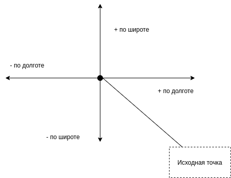
Взять изначальную точку координат, и прибавить к ней число градусов соответствующее расстоянию, необходимому для выборки.

Если соединить эти точки, на которые мы прибавили изначальную координату получится квадрат (простите не ровно нарисовал).

Далее с помощью все той же википедии я открыл для себя несколько формул, и одна из них прямо то что нужно. Это формула вычисления длины градуса. Помните в начале я говорил, что 111 км. это слишком абстрактно из первого решения в вопросе. Так вот, эта формула позволяет вычислять длину градуса непосредственно на конкретной меридиане или параллели, нужно только знать радиус нашего шара. Там же на странице википедии есть предварительно рассчитанные данные, по которым можно будет проверить свою формулу

Расчеты

Приступаем к расчетам. Из открытых источников нам известно, что:

• Средний радиус Земли R = 6371210 м.

• Экваториальный радиус Земли R_Э = 6378,245 м.

• Полярный радиус Земли R_П = 6356,830 м.

Я для расчетов взял средний радиус. Естественно нужно помнить, что земля все-таки не идеальная сфера, поэтому погрешность есть и в этих расчетах, но для нашей задачи это допустимая погрешность.

Я написал небольшой код для проверки вычислений, и для того, чтобы я мог взять числа и проверить их на реальных данных.

Код для проверки

const EART_RADIUS = 6371210; //Радиус земли
const DISTANCE = 20000; //Интересующее нас расстояние

//https://en.wikipedia.org/wiki/Longitude#Length_of_a_degree_of_longitude
function computeDelta(degrees) {
  return Math.PI / 180 * EART_RADIUS * Math.cos(deg2rad(degrees));
}

function deg2rad(degrees) {
  return degrees * Math.PI / 180;
}

const latitude = 55.460531; //Интересующие нас координаты широты
const longitude = 37.210488; //Интересующие нас координаты долготы

const deltaLat = computeDelta(latitude); //Получаем дельту по широте
const deltaLon = computeDelta(longitude); // Дельту по долготе

const aroundLat = DISTANCE / deltaLat; // Вычисляем диапазон координат по широте
const aroundLon = DISTANCE / deltaLon; // Вычисляем диапазон координат по долготе

console.log(aroundLat, aroundLon);

В коде я сразу установил константу расстояния, радиуса земли и принял решение все считать в метрах, поскольку данные я нашел в метрах и лень было разделить их на 1000, да и в метрах казалось, что точность немного выше, чем в километрах с округлением.

Суть этого кода в следующем. Мы не забываем перевести градусы координат в радианы, поскольку формула из википедии рассчитана на радианы. Мы вычисляем дельту ширины и долготы одинаково по одной и той же формуле, поскольку мы условились что у нас идеальный шар и эта погрешность нам допустима. С помощью формулы мы узнаем сколько градусов у нас в одном километре, а дальше простая пропорция.

1 градус — 63046.689652997775 метров
X градусов — 200000 метров

select
	name,
	latitude,
	longitude
from
	villages
where
	latitude between 55.460531 - 0.31722522007226484 and 55.460531 + 0.31722522007226484
	and longitude between 37.210488 - 0.22583381380662185 and 37.210488 + 0.22583381380662185;

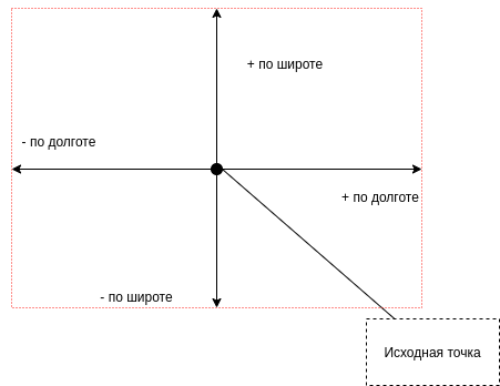
Ну и в моей выборке оказалось 7 объектов. Конечно я взял эту выборку и проверил координаты с помощью линейки на Яндекс Картах. В моем случае все попали в радиус обозначенных 20км. Но мы же помним, что взяли квадрат, а не окружность для вычисления?! Я там даже схему нарисовал в начале, что за квадрат. Итак, если сделать окружность, внутри этого квадрата, она как раз будет радиусом примерно те же 20 км.

Я добавил картинку для наглядности. Видно, что если высота квадрата 40 км, и в нем окружность, то радиус ее тоже будет соответствовать 20 км. Остаются лишние области — углы квадрата, которые я закрасил зеленым. Это то что у нас может попасть в выборку, но они уже не соответствуют именно радиусу в 20 км. Т.е. это лишние данные. И вот тут приходит на помощь та самая формула, о которой я говорил в начале — Расчет расстояния между координатами. С помощью этой формулы можно сравнить исходную точку с координатами из выборки и отсечь те, что будут превышать те самые 20 км, поставленные в задаче.

Итог

Задача решена. Алгоритм придуман. Осталось упаковать это в «красивый» и «чистый» код, чтобы все было по феншую. Надеюсь статья была полезной, потому что когда я искал решения задачи, я наткнулся на множество формул, на множество идей, но не нашел места, где это было бы собрано вот так, как попытался собрать я в рамках данной статьи.

Ссылки

Расчет длины градуса

Расчет дистанции между координатами на сфере

Статья, которая помогла вникнуть в тему расчетов

Тоже полезная статья, в ней есть данные для расчетов

Я почему-то понял вопрос не правильно и подумал про N ближайших точек. Как уже ответил господин @AnT разбиение Вороного для этого намного лучше подойдет, собрал пример на d3.js в котором реализовано разбиение Вороного:

Для поиска нескольких точек можно воспользоваться деревьями

Есть квадродерево алгоритмы на нем достаточно просты и есть готовые реализации.

Вот пример использования d3-quadtree от автора d3.js

желтые — узлы которые обошел алгоритм поиска

красные — найденные ближайшие узлы узлы

Вот пример испольлзующий kd-дерево и поиск ближайших соседей из этого примера на d3.v3 под последнюю версию d3.v5

From Wikipedia, the free encyclopedia

Nearest neighbor search (NNS), as a form of proximity search, is the optimization problem of finding the point in a given set that is closest (or most similar) to a given point. Closeness is typically expressed in terms of a dissimilarity function: the less similar the objects, the larger the function values.

Formally, the nearest-neighbor (NN) search problem is defined as follows: given a set S of points in a space M and a query point q ∈ M, find the closest point in S to q. Donald Knuth in vol. 3 of The Art of Computer Programming (1973) called it the post-office problem, referring to an application of assigning to a residence the nearest post office. A direct generalization of this problem is a k-NN search, where we need to find the k closest points.

Most commonly M is a metric space and dissimilarity is expressed as a distance metric, which is symmetric and satisfies the triangle inequality. Even more common, M is taken to be the d-dimensional vector space where dissimilarity is measured using the Euclidean distance, Manhattan distance or other distance metric. However, the dissimilarity function can be arbitrary. One example is asymmetric Bregman divergence, for which the triangle inequality does not hold.^[1]

Applications[edit]

The nearest neighbour search problem arises in numerous fields of application, including:

• Pattern recognition – in particular for optical character recognition
• Statistical classification – see k-nearest neighbor algorithm
• Computer vision – for point cloud registration^[2]
• Computational geometry – see Closest pair of points problem
• Databases – e.g. content-based image retrieval
• Coding theory – see maximum likelihood decoding
• Semantic Search
• Data compression – see MPEG-2 standard
• Robotic sensing^[3]
• Recommendation systems, e.g. see Collaborative filtering
• Internet marketing – see contextual advertising and behavioral targeting
• DNA sequencing
• Spell checking – suggesting correct spelling
• Plagiarism detection
• Similarity scores for predicting career paths of professional athletes.
• Cluster analysis – assignment of a set of observations into subsets (called clusters) so that observations in the same cluster are similar in some sense, usually based on Euclidean distance
• Chemical similarity
• Sampling-based motion planning

Methods[edit]

Various solutions to the NNS problem have been proposed. The quality and usefulness of the algorithms are determined by the time complexity of queries as well as the space complexity of any search data structures that must be maintained. The informal observation usually referred to as the curse of dimensionality states that there is no general-purpose exact solution for NNS in high-dimensional Euclidean space using polynomial preprocessing and polylogarithmic search time.

Exact methods[edit]

Linear search[edit]

The simplest solution to the NNS problem is to compute the distance from the query point to every other point in the database, keeping track of the «best so far». This algorithm, sometimes referred to as the naive approach, has a running time of O(dN), where N is the cardinality of S and d is the dimensionality of S. There are no search data structures to maintain, so the linear search has no space complexity beyond the storage of the database. Naive search can, on average, outperform space partitioning approaches on higher dimensional spaces.^[4]

The absolute distance is not required for distance comparison, only the relative distance. In geometric coordinate systems the distance calculation can be sped up considerably by omitting the square root calculation from the distance calculation between two coordinates. The distance comparison will still yield identical results.

Space partitioning[edit]

Since the 1970s, the branch and bound methodology has been applied to the problem. In the case of Euclidean space, this approach encompasses spatial index or spatial access methods. Several space-partitioning methods have been developed for solving the NNS problem. Perhaps the simplest is the k-d tree, which iteratively bisects the search space into two regions containing half of the points of the parent region. Queries are performed via traversal of the tree from the root to a leaf by evaluating the query point at each split. Depending on the distance specified in the query, neighboring branches that might contain hits may also need to be evaluated. For constant dimension query time, average complexity is O(log N) ^[5] in the case of randomly distributed points, worst case complexity is O(kN^(1-1/k))^[6]
Alternatively the R-tree data structure was designed to support nearest neighbor search in dynamic context, as it has efficient algorithms for insertions and deletions such as the R* tree.^[7] R-trees can yield nearest neighbors not only for Euclidean distance, but can also be used with other distances.

In the case of general metric space, the branch-and-bound approach is known as the metric tree approach. Particular examples include vp-tree and BK-tree methods.

Using a set of points taken from a 3-dimensional space and put into a BSP tree, and given a query point taken from the same space, a possible solution to the problem of finding the nearest point-cloud point to the query point is given in the following description of an algorithm

. (Strictly speaking, no such point may exist, because it may not be unique. But in practice, usually we only care about finding any one of the subset of all point-cloud points that exist at the shortest distance to a given query point.) The idea is, for each branching of the tree, guess that the closest point in the cloud resides in the half-space containing the query point. This may not be the case, but it is a good heuristic. After having recursively gone through all the trouble of solving the problem for the guessed half-space, now compare the distance returned by this result with the shortest distance from the query point to the partitioning plane. This latter distance is that between the query point and the closest possible point that could exist in the half-space not searched. If this distance is greater than that returned in the earlier result, then clearly there is no need to search the other half-space. If there is such a need, then you must go through the trouble of solving the problem for the other half space, and then compare its result to the former result, and then return the proper result. The performance of this algorithm is nearer to logarithmic time than linear time when the query point is near the cloud, because as the distance between the query point and the closest point-cloud point nears zero, the algorithm needs only perform a look-up using the query point as a key to get the correct result.

Approximation methods[edit]

An approximate nearest neighbor search algorithm is allowed to return points whose distance from the query is at most times the distance from the query to its nearest points. The appeal of this approach is that, in many cases, an approximate nearest neighbor is almost as good as the exact one. In particular, if the distance measure accurately captures the notion of user quality, then small differences in the distance should not matter.^[8]

Greedy search in proximity neighborhood graphs[edit]

Proximity graph methods (such as HNSW^[9]) are considered the current state-of-the-art for the approximate nearest neighbors search.^[9][10][11]

The methods are based on greedy traversing in proximity neighborhood graphs in which every point is uniquely associated with vertex . The search for the nearest neighbors to a query q in the set S takes the form of searching for the vertex in the graph .
The basic algorithm – greedy search – works as follows: search starts from an enter-point vertex by computing the distances from the query q to each vertex of its neighborhood , and then finds a vertex with the minimal distance value. If the distance value between the query and the selected vertex is smaller than the one between the query and the current element, then the algorithm moves to the selected vertex, and it becomes new enter-point. The algorithm stops when it reaches a local minimum: a vertex whose neighborhood does not contain a vertex that is closer to the query than the vertex itself.

The idea of proximity neighborhood graphs was exploited in multiple publications, including the seminal paper by Arya and Mount,^[12] in the VoroNet system for the plane,^[13] in the RayNet system for the ,^[14] and in the Metrized Small World^[15] and HNSW^[9] algorithms for the general case of spaces with a distance function. These works were preceded by a pioneering paper by Toussaint, in which he introduced the concept of a relative neighborhood graph.^[16]

Locality sensitive hashing[edit]

Locality sensitive hashing (LSH) is a technique for grouping points in space into ‘buckets’ based on some distance metric operating on the points. Points that are close to each other under the chosen metric are mapped to the same bucket with high probability.^[17]

Nearest neighbor search in spaces with small intrinsic dimension[edit]

The cover tree has a theoretical bound that is based on the dataset’s doubling constant. The bound on search time is O(c¹² log n) where c is the expansion constant of the dataset.

Projected radial search[edit]

In the special case where the data is a dense 3D map of geometric points, the projection geometry of the sensing technique can be used to dramatically simplify the search problem.
This approach requires that the 3D data is organized by a projection to a two-dimensional grid and assumes that the data is spatially smooth across neighboring grid cells with the exception of object boundaries.
These assumptions are valid when dealing with 3D sensor data in applications such as surveying, robotics and stereo vision but may not hold for unorganized data in general.
In practice this technique has an average search time of O(1) or O(K) for the k-nearest neighbor problem when applied to real world stereo vision data.
^[3]

Vector approximation files[edit]

In high-dimensional spaces, tree indexing structures become useless because an increasing percentage of the nodes need to be examined anyway. To speed up linear search, a compressed version of the feature vectors stored in RAM is used to prefilter the datasets in a first run. The final candidates are determined in a second stage using the uncompressed data from the disk for distance calculation.^[18]

Compression/clustering based search[edit]

The VA-file approach is a special case of a compression based search, where each feature component is compressed uniformly and independently. The optimal compression technique in multidimensional spaces is Vector Quantization (VQ), implemented through clustering. The database is clustered and the most «promising» clusters are retrieved. Huge gains over VA-File, tree-based indexes and sequential scan have been observed.^[19][20] Also note the parallels between clustering and LSH.

Variants[edit]

There are numerous variants of the NNS problem and the two most well-known are the k-nearest neighbor search and the ε-approximate nearest neighbor search.

k-nearest neighbors [edit]

k-nearest neighbor search identifies the top k nearest neighbors to the query. This technique is commonly used in predictive analytics to estimate or classify a point based on the consensus of its neighbors. k-nearest neighbor graphs are graphs in which every point is connected to its k nearest neighbors.

Approximate nearest neighbor[edit]

In some applications it may be acceptable to retrieve a «good guess» of the nearest neighbor. In those cases, we can use an algorithm which doesn’t guarantee to return the actual nearest neighbor in every case, in return for improved speed or memory savings. Often such an algorithm will find the nearest neighbor in a majority of cases, but this depends strongly on the dataset being queried.

Algorithms that support the approximate nearest neighbor search include locality-sensitive hashing, best bin first and balanced box-decomposition tree based search.^[21]

Nearest neighbor distance ratio[edit]

Nearest neighbor distance ratio does not apply the threshold on the direct distance from the original point to the challenger neighbor but on a ratio of it depending on the distance to the previous neighbor. It is used in CBIR to retrieve pictures through a «query by example» using the similarity between local features. More generally it is involved in several matching problems.

Fixed-radius near neighbors[edit]

Fixed-radius near neighbors is the problem where one wants to efficiently find all points given in Euclidean space within a given fixed distance from a specified point. The distance is assumed to be fixed, but the query point is arbitrary.

All nearest neighbors[edit]

For some applications (e.g. entropy estimation), we may have N data-points and wish to know which is the nearest neighbor for every one of those N points. This could, of course, be achieved by running a nearest-neighbor search once for every point, but an improved strategy would be an algorithm that exploits the information redundancy between these N queries to produce a more efficient search. As a simple example: when we find the distance from point X to point Y, that also tells us the distance from point Y to point X, so the same calculation can be reused in two different queries.

Given a fixed dimension, a semi-definite positive norm (thereby including every L^p norm), and n points in this space, the nearest neighbour of every point can be found in O(n log n) time and the m nearest neighbours of every point can be found in O(mn log n) time.^[22][23]

See also[edit]

References[edit]

Citations[edit]

Sources[edit]

• Andrews, L. (November 2001). «A template for the nearest neighbor problem». C/C++ Users Journal. 19 (11): 40–49. ISSN 1075-2838.
• Arya, S.; Mount, D.M.; Netanyahu, N. S.; Silverman, R.; Wu, A. Y. (1998). «An Optimal Algorithm for Approximate Nearest Neighbor Searching in Fixed Dimensions». Journal of the ACM. 45 (6): 891–923. CiteSeerX 10.1.1.15.3125. doi:10.1145/293347.293348. S2CID 8193729.
• Beyer, K.; Goldstein, J.; Ramakrishnan, R.; Shaft, U. (1999). «When is nearest neighbor meaningful?». Proceedings of the 7th ICDT.
• Chen, Chung-Min; Ling, Yibei (2002). «A Sampling-Based Estimator for Top-k Query». ICDE: 617–627.
• Samet, H. (2006). Foundations of Multidimensional and Metric Data Structures. Morgan Kaufmann. ISBN 978-0-12-369446-1.
• Zezula, P.; Amato, G.; Dohnal, V.; Batko, M. (2006). Similarity Search – The Metric Space Approach. Springer. ISBN 978-0-387-29146-8.

Further reading[edit]

• Shasha, Dennis (2004). High Performance Discovery in Time Series. Berlin: Springer. ISBN 978-0-387-00857-8.

External links[edit]

• Nearest Neighbors and Similarity Search – a website dedicated to educational materials, software, literature, researchers, open problems and events related to NN searching. Maintained by Yury Lifshits
• Similarity Search Wiki – a collection of links, people, ideas, keywords, papers, slides, code and data sets on nearest neighbours

Рассмотрим точку $%M(x_0, y_0)$% и произвольную функцию $%y = f(x)$%. Тогда назовем расстоянием от точки $%M$% до функции $%y=f(x)$% некоторый отрезок $%MK$%, где $%K = (x_1, f(x_1))$%. Наименьшим расстоянием — такое расстояние, для которого $%|MK|$% наименьший. Тогда, если мы хотим минимизировать $%|MK|$%, мы можем минимизировать $%p = |MK|^2 = (x_1 — x_0)^2 + (f(x_1) — y_0)^2$%. Это несложно сделать, просто взяв производную и найдя минимум данной функции, зависящей только от параметра $%x_1$%.

Покажу на примере:
$%y = sqrt{x}$%, $%M(2;0)$%. Рассмотрим $%p = (x-2)^2 + (sqrt{x})^2 = x^2-4x+4+x=x^2-3x+4$%. Понятно, что минимум данной функции находится в точке $%x_1 = frac{3}{2}$%. Соответственно, наиболее близкая точка на графике данной функции к точке $%M$% будет точка $%(frac{3}{2}; sqrt{frac{3}{2}})$%.