Коэффициент
сверхсжимаемости газов – это отношение
объема υ при заданных значениях Р
и Т к
объему этого газа, определенному при
идентичных Р и
Т по
законам идеального газа υид.
Коэффициент сверхсжимаемости
характеризует отклонение объема
реального газа от объема “идеального”.
Формула, связывающая основные
параметры газа – объем, давление и
температуру, называется уравнением
состояния газа. Уравнение состояния
идеального газа получено из условия
отсутствия межмолекулярных
взаимодействий и без учета объема самих
молекул и имеет вид
υид=nRT/P (2.19)
где n
– число молей газа; R
– универсальная газовая
постоянная; Т и Р –
температура и давление
газа.
Уравнение состояния
реального газа может быть представлено
в виде:
υ=nZRT/P (2.20)
Универсальная
газовая постоянная R
выражает работу одного моля газа при
повышении его температуры на один градус
и в системе СИ имеет размерность
Дж/кмоль·град.
Коэффициент
сверхсжимаемости газа Z
зависит от состава газа, давления и
температуры. Значение коэффициента
может быть определено графическим и
аналитическим способами. Способ
определения следует выбирать, исходя
из требуемой точности его значения.
Наиболее простым способом определения
Z
является графический. Для
определения Z
природных газов, содержащих не более
2% (мольных) высококипящих углеводородов
С5+,
2% ароматических углеводородов и около
5% полярных и кислых компонентов, можно
использовать графическую зависимость
Z
от приведенного давления Рпр
и
приведенной температуры Тпр,
показанных
на рисунках
2.4
и 2.5.
На рисунках
2.6÷2.8 приведены
зависимости Z
от Р и
Т для N2,
CO2
и H2S.
При
более высоком содержании в газе
высококипящих углеводородов С5+
и полярных компонентов
коэффициент сверхсжимаемости Z
следует определять с учетом ацентричного
фактора по формуле:
Z=Z(0)+ωсмZ(1) (2.21)
где
Z(0),
Z(1)
– коэффициенты, определяемые из графиков
зависимостей Z(0)
и Z(1)
от приведенных
параметров Рпр
и Тпр,
показанных на рисунках
2.9 и 2.10;
ωсм
– фактор ацентричности, определяемый
по известному составу газа по формуле:
 (2.22)
где
ωi
– фактор ацентричности i-го
компонента, определяемый из таблицы
2.2 или по формуле
(2.6).
Псевдокритические
параметры, необходимые для определения
Рпр
и Тпр,
с помощью которых из
графиков находят Z(0)
и
Z(1),
должны
быть определены в
зависимости от состава газа. Если в газе
количество высококипящих углеводородов
и полярных веществ более 5%, то
псевдокритические параметры должны
быть определены согласно [18]:
Рисунок
2.4 – Зависимость
коэффициента сверхсжимаемости Z
метана от приведенных давления и
температуры.
Рисунок 2.5 –
Зависимость коэффициента
сверхсжимаемости Z
природного газа от приведенных давления
и температуры.

Рисунок 2.6 –
Зависимость коэффициента сверхсжимаемости
Z азота от давления
и температуры.

Рисунок
2.7 – Зависимость
коэффициента сверхсжимаемости Z
углекислого газа от давления и температуры.

Рисунок
2.8 – Зависимость
коэффициента сверхсжимаемости Z
сероводорода от
давления и температуры.

Рисунок
2.9 – Зависимость
коэффициента сверхсжимаемости Z(0)
простых веществ от
приведенных давления и температуры.

Рисунок
2.10 – Зависимость коэффициента
сверхсжимаемости Z(1)
несферических молекул от приведенного
давления и температуры.
Если
в газе содержится более 5% СО2,
то значение Z
должно быть рассчитано следующим
образом:
– по
формулам (2.3) вычисляют псевдокритические
давление Рпк
и температуру Тпк;
– вычисляется
фактор ацентричности смеси ωсм,
исключая из нее СО2,
по формуле:
 (2.23)
– по
известной величине ωугл
и концентрации СО2
в газе из графика, показанного на рисунке
2.11а
и б,
определяется величина
ε, являющейся температурной поправкой
для используемой при расчетах
псевдокритической температуры. При
наличии в газе СО2 и
H2S
значение ε может быть рассчитано и по
формуле:
![]() (2.24)
(2.24)
где А
– суммарные мольные
доли СО2
и H2S
в газе; В –
мольная доля H2S.


Рисунок
2.11 – Зависимость
псевдокритической температурной
поправки ε от концентрации в смеси СО2
и фактора ацентричности ω.
Зная
Рпк,
Тпк
и ω вычисляют новые псевдокритические
параметры:
![]() ;
;
![]() (2.25)
(2.25)

Рисунок
2.12 – Зависимость
псевдокритической температурной
поправки ε от концентрации в смеси СО2
и H2S.
Зная
Рпк,
Тпк
и ω, вычисляют новые
псевдокритические параметры:
По
известным величинам заданных Р
и Т и
вычисленным Р*пк
и Т*пк
рассчитывают приведенные
параметры:
![]()
![]() (2.26)
(2.26)
Используя
графики, приведенные в [18] определяют
Z(0)
и Z(1),
а затем, используя формулу (2.21), вычисляют
значение Z.
При
наличии в газе СО2
и H2S
коэффициент сверхсжимаемости Z
определяется аналогичным образом, с
той лишь разницей, что при вычислении
фактора ацентричности ωугл
по формуле (2.23) из состава газа исключается
не только СО2,
но и H2S.
Если
для определения газов, содержащих кислые
компоненты, т.е. СО2
и H2S,
используются графики, показанные на
рисунках 2.1
и 2.2,
то последовательность расчета выполняется
следующим образом:
– по
формулам (2.3) рассчитываются значения
Рпк
и Тпк;
– по
графикам из рисунка
2.11 находят поправочный
коэффициент ε;
– вычисляются
новые псевдокритические параметры по
формулам
![]() (2.27)
(2.27)
где
xH2S
– мольная доля сероводорода в смеси;
![]() (2.28)
(2.28)
Используя
формулу (2.26), рассчитывают величины Рпр
и Тпр,
а затем по этим приведенным
параметрам из графика в
[18] находят коэффициенты
сверхсжимаемости Z(0)
и Z(1).
По известным Z(0)
и Z(1)
вычисляют Z.
Для
более точных расчетов коэффициент
сверхсжимаемости природных газов Z
должен быть определен по кубическим
уравнениям состояния газов, наиболее
широкое распространение, среди которых
получили уравнения Соаве, Редлиха-Квонга,
Пенга-Робинсона. При этих методах расчета
присутствие в газе кислых компонентов
практически не влияет на величину
погрешности при определении Z,
если расчеты ведутся с учетом коэффициентов
взаимодействия.
Для
определения коэффициента сверхсжимаемости
Z
кубические уравнения состояния
решаются относительно Z.
Имеющее достаточно высокую точность
уравнение Редлиха-Квонга для определения
Z
записывается в виде:
![]() (2.29)
(2.29)
где
асм=∑xiai;
bсм=∑xibi (2.30)
![]() ;
;
![]() (2.31)
(2.31)
Уравнение (2.29) дает
искомую точность для газообразных
компонентов и их смесей. Наличие в смеси
компонентов в жидком состоянии, а также
молекул различного строения резко
увеличивает погрешность расчетов.
Повышение
точности величины Z
при этом возможно путем
введения поправки ΔZ
на Z,
определенной по формуле (2.21).
Наиболее
точно коэффициент сверхсжимаемости Z
определяется из уравнения состояния
Пенга-Робинсона, имеющего относительно
Z
вид:
См.
ниже за таблицей 2.5:
Z3–(l–A)Z2+(A–3B2–2B)Z–(AB–B2–B3)=0, (2.32)
где
A=aP/R2T;
B=bP/RT; (2.33)
 ;
;
 (2.34)
![]() ;
;
![]() (2.35)
(2.35)
![]() ;
;
![]()
(2.36)
Значения
коэффициента Cij
в формуле (2.34)
приведены в таблице
2.5.
Таблица
2.5 – Значение коэффициента Сij
в формуле (2.34)
|
Компоненты газа |
Cij |
||||||||||||
|
N2 |
CO2 |
H2S |
CH4 |
C2H6 |
C3H8 |
n-C4H10 |
n-C5H12 |
n-C6H14 |
n-C7H16 |
n-C8H18 |
n-C9H20 |
n-C10H22 |
|
|
N2 |
0 |
0 |
0,130 |
0,025 |
0,010 |
0,090 |
0,095 |
0,100 |
0,110 |
0,115 |
0,120 |
0,120 |
0,123 |
|
CO2 |
– |
0 |
0,135 |
0,105 |
0,130 |
0,125 |
0,115 |
0,115 |
0,115 |
0,115 |
0,115 |
0,115 |
0,115 |
|
H2S |
– |
– |
0 |
0,070 |
0,085 |
0,080 |
0,075 |
0,070 |
0,060 |
0,060 |
0,060 |
0,060 |
0,055 |
|
CH4 |
– |
– |
– |
0 |
0 |
0,010 |
0,025 |
0,030 |
0,030 |
0,035 |
0,040 |
0,040 |
0,045 |
|
C2H6 |
– |
– |
– |
– |
– |
0,005 |
0,010 |
0,010 |
0,020 |
0,020 |
0,020 |
0,020 |
0,020 |
|
C3H8 |
– |
– |
– |
– |
– |
0 |
0 |
0,005 |
0,005 |
0,005 |
0,005 |
0,005 |
0,005 |
|
n-C4H10 |
– |
– |
– |
– |
– |
– |
0 |
0,005 |
0,005 |
0 |
0 |
0,005 |
0,005 |
|
n-C5H12 |
– |
– |
– |
– |
– |
– |
– |
0 |
0 |
0 |
0 |
0 |
0 |
|
n-C6H14 |
– |
– |
– |
– |
– |
– |
– |
– |
0 |
0 |
0 |
0 |
0 |
|
n-C7H16 |
– |
– |
– |
– |
– |
– |
– |
– |
– |
0 |
0 |
0 |
0 |
|
n-C8H18 |
– |
– |
– |
– |
– |
– |
– |
– |
– |
– |
0 |
0 |
0 |
|
n-C9H20 |
– |
– |
– |
– |
– |
– |
– |
– |
– |
– |
– |
0 |
0 |
|
n-C10H22 |
– |
– |
– |
– |
– |
– |
– |
– |
– |
– |
– |
0 |
0 |
Более простой
вариант
2.
Коэффициент сверхсжимаемости газа
рассчитываем по формуле Пенга –
Робинсона:
![]() ,
,
(2.22)
или
![]() ,
,
где:
![]() ,
,
![]() ,
,
![]() ,
,
![]() ,
,
![]() ,
,
![]() ,
,
![]() ,
,
![]()
Соседние файлы в предмете [НЕСОРТИРОВАННОЕ]
- #
- #
- #
- #
- #
- #
- #
- #
- #
- #
- #
Коэффициент сверхсжимаемости Z реальных газов — это отношение
объемов равного числа молей реального V и идеального Vи газов при одинаковых давлении и
температуре: Z = V/Vи
Значения коэффициентов сверхсжимаемости наиболее надежно
могут быть определены на основе лабораторных исследований пластовых проб газов.
При отсутствии таких исследований прибегают к расчетному методу оценки Z по графику
Г. Брауна. Для пользования графиком необходимо знать приведенные псевдокритическое давление
(давление, соответствующее критической точке перехода газа в жидкое
состояние) и псевдокритическую
температуру (температура, выше которой газ не может быть превращен в жидкость
ни при каком давлении).
Для определения коэффициента
сверхсжимаемости Z реальных газов, представляющих собой ногокомпонентную смесь, находят
средние из значений критических давлений и температур каждого компонента. Эти
средние называются псевдокритическим давлением Рпкр и
псевдокритической температурой Тпкр. Они определяются из соотношений:

где Pкрi, и Tкрi — критические давление и температура i-го
компонента; Xi — доля i-го
компонента в объеме смеси (в долях единицы). Приведенные псевдокритические
давление и температура, необходимые для пользования графиком Брауна,
представляют собой псевдокритические значения, приведенные к конкретным
давлению и температуре (к пластовым, стандартным или каким-либо другим
условиям):
Pпр=Р/Рпкр; Тпр=Т/Тпкр,
где Р и Т— конкретные давление и
температура, для которых определяется Z.
Коэффициент
сверхсжимаемости Z обязательно используется при подсчете запасов газа, прогнозировании
изменения давления в газовой залежи и решении других задач.
ДОБЫЧА И ПЕРЕРАБОТКА НЕФТИ И ГАЗА
УДК 622.279
В. С. Семенякин, А. Е. Калинин
КОЭФФИЦИЕНТ СВЕРХСЖИМАЕМОСТИ ПЛАСТОВОЙ СМЕСИ ГАЗОВ И МЕТОДЫ ЕГО ОПРЕДЕЛЕНИЯ
Коэффициент сверхсжимаемости газа Z характеризует отклонение объема реального газа от объема «идеального». Этот коэффициент зависит от состава смеси пластового газа, давления и температуры. Определение значения коэффициента сверхсжимаемости обычно осуществляют графоаналитическим способом, предложенным в [1]. Данный способ нашел широкое распространение в практике анализа состояния природных газов различных месторождений, имеющих аномально высокие и нормальные пластовые давление и температуру. Тем не менее следует отметить, что графики в [1- 3 и др.] не отражают поведение реальных природных газов газоконденсатных месторождений, т. к. построены для отдельных компонентов газа. Это потребовало введения поправок к значениям абсолютного давления при наличии в смеси пластового газа сероводорода, азота и диоксида углерода [2]. Однако даже при введении поправок возникали трудности в определении расхода и плотности газа, что, очевидно, было связано с погрешностями при оценке Z, а также с протекающими одновременно процессами ретроградной конденсации и испарения [4]. По этой причине оставались нерешенными проблемы, связанные с определением пластового и забойного давления, рабочих параметров подъемника и т. д.
В связи с вышеизложенным на Астраханском газоконденсатном месторождении (АГКМ) были проведены широкомасштабные исследования на работающих и остановленных скважинах с целью определить зависимость Z от давления и температуры по плотности газа, находящегося в фонтанном подъемнике и на сепарационных установках. Затем была проведена оценка математического ожидания среднего значения давления в каждом интервале подъемника, а также рассчитаны границы 95 %-го доверительного интервала для оценки математического ожидания в пределах 34,5-36,7 МПа, соответствующие давлениям в середине подъемника.
По среднестатистическому составу газа сепарации и пластового газа АГКМ, а также среднестатистическим замеренным значениям давления Р и температуры Т по высоте подъемника (от устья до забоя скважин с шагом 500 м) по аналитической зависимости, приведенной в [2, 5],
Рг = РстРТст/РатТ2
были рассчитаны значения Z и нанесены на график в функции давления (рис. 1).
(1)
г
* Для газа сепарации ■ Для пластового газа
Рис. 1
Как видно из рис. 1, в доверительном интервале значения Z для газа сепарации и пластового газа близки (расхождение не превышает 0,5 %).
Основываясь на сделанном предположении, расчет среднего значения Zcр для газа в подъемнике осуществляли в определенной последовательности. Сначала строится модель, по которой в дальнейшем будет оцениваться значение ^ Для построения модели используется аналитическая зависимость [5], в которой приняты усредненные значения давления Рср и температуры Тср в подъемнике, определяемые из выражений:
РСр = 0,6717Рп/Ркр ; (2)
Тср = 0,71892Тп/ТКр , (3)
где Рп, Тп — давление, МПа, и температура, К, в подъемнике; Ркр, Ткр — критические давление, МПа, и температура, К, газовой фазы в подъемнике.
По результатам замеров давления и температуры в подъемнике скважин АГКМ глубинными манометрами и термометрами оценивается математическое ожидание значений давления и температуры на фиксированных глубинах:
М(Р) = Р п г, (4)
М(Тг) = Т ш, г = 0, 1, 2, …, Ы, (5)
где М — символ «оценка математического ожидания»; г — порядковый номер отметок (начиная от устья скважины), на которых производится замер давления и температуры в подъемнике скважины (расстояние между соседними отметками равно 500 м); Р пг , Т пг — средние значения давления и температуры в подъемнике на г-й отметке.
По выборке с объемом п = 75 из значений Ркр и Ткр для газа сепарации, полученных при исследовании скважин, были рассчитаны среднестатистические значения параметров Ркрг.с = 5,83215 МПа, Ткргс = 258,7831 К (значения Ркр и Ткр для газа сепарации распределены по нормальному закону при уровне значимости равном 0,05).
По полученным среднестатистическим значениям Рп, Тп, Ркр г.с , Ткргс и аналитической зависимости [5] были рассчитаны значения Zг.сг■ в подъемнике для каждой г-й отметки измерения.
На заключительном этапе построения модели осуществили подбор наилучшей (в смысле точности аппроксимации) регрессионной зависимости между Zг.c и Р. Так, в качестве рабочей модели был принят полином второй степени со среднеквадратичным отклонением равным 0,003:
г ср = 0,092546 + 3,183478 • 10-2 Рп — 2,594809 • 10-4 Рп2, (6)
по которому определили значения Z в подъемнике скважин АГКМ в интервале давления 25-45 МПа.
При дальнейшей эксплуатации месторождения и снижении пластового давления среднее давление в подъемнике также будет падать. Как видно из рис. 1, при снижении давления вплоть до 25 МПа расхождение между значениями Z для газа сепарации и пластового газа остается постоянным и не превышает 5 %, что позволяет использовать уравнение (6) для оценки Z
__ /V
до Рср = 25 МПа, при котором г ср = 0,726.
Проведем оценку коэффициента Z в зависимости от плотности смеси газов, воспользовавшись данными состава газа различных месторождений, приведенными в [2], при абсолютном давлении 20, 30, 40, 50, 60, 70 МПа с закреплённой температурой 293, 333, 383 К и сопоставим с найденными значениями Z по уравнению (6).
Полученные зависимости приведены на рис. 2 и 3.
Z = Хр) при Т = 293 К
Z = /р) при Т = 333 К
в
Плотность смеси газов
Z = Хр) при Т = 383 К
+ 20 МПа; О 30 МПа; □ 40 МПа; 50 МПа; Ж 60 МПа; • 70 МПа
Рис. 2
а
б
1
Z = Др) при Р = 20 МПа
Z = Др) при Р = 30 МПа
Плотность смеси газов
Z = Др) при Р = 40 МПа
Рис. 3
а
Z
б
Z
в
1,3
Z
1,2
1,1
0,6 0,65 0,7 0,75 0,8 0,85 0,9 0,95 1 1,05
г I = /(р) при Р = 50 МПа
I = /(р) при Р = 60 МПа
Плотность смеси газов
I = /(р) при Р = 70 МПа
д
I
е
Продолжение рис. 3
Расчетные значения !, найденные по уравнению (6), были сопоставлены с данными коэффициента Z для скважин АГКМ при одних и тех же значениях давлений и температур и оказались близкими (ошибка не превышает 0,1 %).
Графики на рис. 2 и 3 позволяют наглядно представить, каким превращениям подвергается пластовая смесь газа при его притоке к скважине, подъеме на дневную поверхность и при транспорте при изменении термобарических условий. Кроме того, они позволяют оперативно определять коэффициент сверхсжимаемости газа по известной плотности пластового газа, не прибегая к сложным методам его определения через приведенные давления и температуры. Представленные зависимости Z = /(рг), в отличие от рекомендованных в известных литературных источниках, расширяют диапазон оценки Z для любых газовых, нефтяных или газоконденсатных месторождений.
СПИСОК ЛИТЕРАТУРЫ
1. Руководство по добыче, транспорту и переработке природного газа / Д. Катц, Д. Корнелл, Р. Кобая-ши и др. — М.: Недра, 1965. — 676 с.
2. Руководство по исследованию скважин / А. И. Гриценко, З. С. Алиев, О. М. Ермилов. — М.: Наука,
1995. — 523 с.
3. Вяхирев Р. И. Теория и опыт добычи газа. — М.: Недра, 1998. — 479 с.
4. Панфилов М. Б. Гидродинамика процессов в газоконденсатном пласте и проблема их регулирования // Газовая промышленность. — 1997. — № 7. — С. 58-61.
5. Плотников В. М., Подрешетников В. А., Тетеревятников Л. Н. Приборы и средства учета природного газа и конденсата. — Л.: Недра, 1989. — 238 с.
Статья поступила в редакцию 9.10.2008
OVERPRESSURE COEFFICIENT OF BEDDED GAS MIXTURE AND METHODS OF ITS DEFINITION
V. S. Semenyakin, А. Е. Kalinin
The widespread estimation method of overpressure coefficient of gases Z is based on the definition of reduced pressure and temperature with the subsequent determination of this factor according to Catts’s nomogram. However, the given method does not take into account the influence of sour components such as hydrogen sulphide and carbon dioxide contained in the mixture of gases that complicates its application. On the basis of an average structure of separation gas and bedded gas taken from Astrakhan gas-condensate field (AGCF) the dependence Z on the pressure, applied only for the given field, has been found out. In this connection a new method of estimation Z on the normal density of the mixture of gases in a wide range of pressure and temperature changes is offered. The values Z for bedded gas from AGCF found by calculated and graphic methods, have shown a good coincidence of magnitudes. Thus, the estimation method Z for mixture of various components of gas may be recommended for application in practice.
Key words: overpressure coefficient of gas, gas-condensate field, bedded pressure and temperature, resulted pressure and temperature, density of gas mixtures.
МИНИСТЕРСТВО
ОБРАЗОВАНИЯ И НАУКИ РОССИЙСКОЙ ФЕДЕРАЦИИ
Политехнический
институт (филиал) федерального государственного автономного образовательного
учреждения высшего профессионального образования «Северо-Восточный федеральный
университет
имени
М. К. Аммосова» в г. Мирном
Горный
факультет
Кафедра
Горного
и нефтегазового дела
Практическая
работа №1
По
дисциплине «Технология эксплуатации газовых скважин»
Тема:
«Выбор методики расчета коэффициента сверхсжимаемости газа»
Вариант
№12
Выполнил: ст. гр. ДГ12-5
Проверил:
Мирный,
2015
Содержание
1. Коэффициент сверхсжимаемости. Методы
определения коэффициента сверхсжимаемости 3
2. Определение
коэффициента сверхжимаемости по графику Брауна — Катца. 4
3. Определение
коэффициента сверхсжимаемости уравнением состояния Пенга — Робинсона 6
Вывод.. 8
Список литературы.. 9
1. Коэффициент сверхсжимаемости. Методы
определения коэффициента сверхсжимаемости
2. Определение
коэффициента сверхжимаемости по графику Брауна — Катца
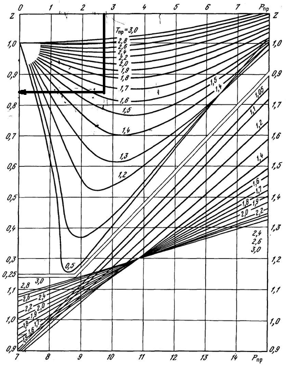
Рис. 1. Зависимость коэффициента
сверхсжимаемости Z природного газа
от приведенных давления и температуры.
Pпл=12,65 Тпл=336,15
Коэффициент сверхсжимаемости по графику
Брауна – Катца: z = 0,847
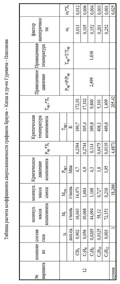
Проверим полученный ответ по уравнению
Гуревича – Платонова:
![]() =
=
0,85
3.
Определение коэффициента сверхсжимаемости уравнением
состояния Пенга — Робинсона

![]()
Находим
коэффициенты входящие в уравнение Пенга-Робинсона:
![]() =
=
0,4129
![]() =
=
0,783
 =
=
2,846 * 1011
![]() =
=
2,228 * 1011
![]() =
=
28348,862
![]() =
=
0,361144

Приводим
уравнение Пенга – Робинса к виду:
![]()
где,
![]()
![]()
![]()
Построим график для определения
коэффициента сверхсжимаемости зависимости ![]() от
от
![]() )
)
|
zi |
f(zi) |
|
0,25 |
-0,05288 |
|
0,35 |
-0,07243 |
|
0,45 |
-0,08841 |
|
0,55 |
-0,09483 |
|
0,65 |
-0,08568 |
|
0,75 |
-0,05496 |
|
0,85 |
0,003322 |
|
0,95 |
0,095175 |
|
1,05 |
0,226596 |
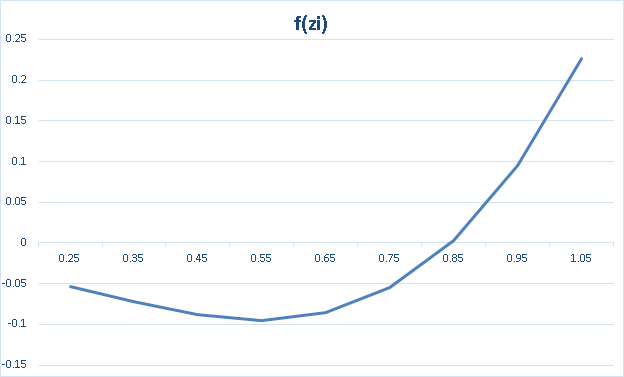
По
данному графику мы можем увидеть, что линия пересекает 0 в точке 0,85
следовательно Z = 0,85
Вывод
В ходе проведенной
работы мы выяснили, что найти коэффициент сверхсжимаемости можно различными
методами, но наиболее эффективный и точный из них, уравнение Гуревича-Платонова
Z
= 0,85. А в графиках мы можем только приблизительно определить величину.
Список
литературы
1.
Алиев З.С., Бондаренко В.В. “Руководство
по проектированию разработки газовых и газонефтяных месторождений”. г. Печора
Изд. “Печорское время”, 2002 г., 894 c.
2.
Балыбердина И.Т. “Физические методы
переработки и использования газа”, М.: “Недра”, 1988
г., 248 с.
3.
Бекиров Т.М., Ланчаков Г.А. “Технология
обработки газа и конденсата”, М.: “Недра”, 1999
г., 596 с.
Production engineering formulas and calculations
Cenk Temizel, … Luigi A. Saputelli, in Formulas and Calculations for Petroleum Engineering, 2019
4.62 Pressure drop across perforations in gas wells
Input(s)
-
qg: Gas Flow Rate through Perforation (bbl/d)
-
n: Number of Perforations (dimensionless)
-
μg: Gas Viscosity (cP)
-
Z: Gas Supercompressibility Factor (dimensionless)
-
T: Formation Temperature (R°)
-
Lp: Perforation Length (ft)
-
kpd: Perforation Damaged Zone Permeability (mD)
-
rp: Perforation Radius (ft)
-
rpd: Perforation Damaged Zone Radius (ft)
-
γg: Gas Specific Gravity (air = 1.0)
Output(s)
-
psf: Pressure at the Sandface (psi)
-
pwb: Pressure in the Wellbore (psi)
-
βpd: Velocity Coefficient of Turbulence Factor (1/ft)
Formula(s)
psf2−pwb2=A·qgn+B·qgn2
A=1.424·103·μgZTLpkpdInrpdrp
B=3.1610−12βpdγgZTLp21rp−1rpd
βpd=2.331010k−1.201
Reference: Bell, W. T., Sukup, R. A., & Tariq, S. M. (1995). Perforating. Henry L. Doherty Memorial Fund of AIME, Society of Petroleum Engineers, Page: 62.
Read full chapter
URL:
https://www.sciencedirect.com/science/article/pii/B9780128165089000044
Gas—Compression
Mark J. Kaiser, E.W. McAllister, in Pipeline Rules of Thumb Handbook (Ninth Edition), 2023
Estimate horsepower required to compress natural gas
To estimate the horsepower to compress a million cubic ft of gas per day (MMcfd), use the following formula:
BHP/MMcfd=RR+RJ(5.16+124Log R0.97−0.03R)
where
-
R = Compression ratio. Absolute discharge pressure divided by absolute suction pressure,
-
J = Supercompressibility factor—assumed 0.022 per 100 psia suction pressure.
Example
How much horsepower should be installed to raise the pressure of 10 million cu ft of gas per day from 185.3 psi to 985.3 psi?
Solution
This gives absolute pressures of 200 and 1000.
R=1000200=5.0
Substituting in the formula:
BHP/MMcfd=5.05.0+5×0.044×5.15+124×.6990.97−0.03×5=106.5hp=BHP for 10MMcfd=1065hp

where the suction pressure is about 400 psia, and the brake horsepower per MMcfd can be read from the chart.
The previous formula may be used to calculate horsepower requirements for various suction pressures and gas physical properties to plot a family of curves.
Read full chapter
URL:
https://www.sciencedirect.com/science/article/pii/B9780128227886000049
Volumetric Measurement
Dr.Boyun Guo, Dr.Ali Ghalambor, in Natural Gas Engineering Handbook (Second Edition), 2005
10.2.1 Orifice Equation
The basis for the orifice-meter equation is the first law of thermal dynamics. Derivation of the equation can be found in a number of publications such as that by Ikoku (1984). For the calculation of the quantity of gas, AGA (1956) recommends the formula:
(10.1)qh=C’hwpf
where
-
qh = quantity rate of flow at base conditions, cfh
-
C″ = orifice flow constant
-
hw = differential pressure in inches of water at 60 °F
-
pf = absolute static pressure, psia
The orifice flow constant C″ is expressed in the following equation:
(10.2)C’=(Fb)(Fr)(Y)(Fpb)(Ftb)(Ftf)(Fg)(Fpv)(Fm)(F1)(Fa)
where
-
Fb = basic orifice factor, cfh
-
Fr = Reynolds number factor
-
Y = expansion factor
-
Fpb = pressure base factor
-
Ftb = temperature base factor
-
Ftf = flowing temperature factor
-
Fg = specific gravity factor
-
Fpv = supercompressibility factor
-
Fm = manometer factor for mercury meter
-
F1 = gauge location factor
-
Fa = orifice thermal expansion factor
The basic orifice factor, Fb, is dependent on the location of the taps, the internal diameter of the run, and the size of the orifice. Tables for the basic orifice factor are presented in Appendix C of this book.
The Reynolds number factor, Fr, is dependent on the pipe diameter and the viscosity, density, and velocity of the gas. It is expressed as:
(10.3)Fr=1+bhwpf
where the values of b are given in Appendix C of this book.
The expansion factor, Y, depends on the expansion of gas through the orifice. The density of the stream changes because of the pressure drop and the adiabatic temperature change. The expansion factor Y corrects for the variation in density. It is a function of the differential pressure, the absolute pressure, the diameter of the pipe, the diameter of the orifice, and the type of taps. Tables for Y values are presented in Appendix C of this book. The pressure base factor, Fpb, is a direct application of Boyle’s law in the correction for the difference in base from 14.73 psia. The pressure base is set by contract:
(10.4)Fpb=14.73pb
The temperature base factor, Ftb, would be used in a direct application of Charles’s law to correct for the base temperature change from 60 °F. Gas measured at one base temperature will have a different calculated volume if it is sold to a customer on a different base. That is, if the gas is measured at a base temperature of 60 °F and sold at a base temperature of 70 °F, the company must correct the volume to the contract temperature or, in this case, lose money. It is clear that the absolute temperature of the base (60 °F) divided by the absolute temperature of the contract will give a factor that should be applied to correct the meter reading to the terms of the contract temperature.
(10.5)Ftb=tb+460520
The flowing temperature factor, Ftf, corrects the effects of temperature variation. The flowing temperature has two effects on the volume. A higher temperature means a lighter gas so that flow will increase. Also, a higher temperature causes the gas to expand, which reduces the flow. The combined effect is to cause the quantity of flow of a gas to vary inversely as the square root of the absolute flow temperature. The Ftf is usually applied to the average temperature during the time gas is passing. The temperature may be taken by recording charts or by periodic indicating thermometer readings.
(10.6)Ftf=520t+460
where t = fluid temperature, °F
The specific gravity factor, Fg, is used to correct for changes in the specific gravity and should be based on the actual flowing specific gravity of the gas as determined by test. The specific gravity may be determined continuously by a recording gravitometer or by gravity balance on a daily, weekly, or monthly schedule, or as often as necessary to meet conditions of the contract. The basic orifice factor is determined by air with a specific gravity of 1. With a given force applied on a gas, a larger quantity of lightweight gas can be pushed through an orifice than a heavier gas. To make the basic orifice factor usable for any gas, the proper correction for the specific gravity of the gas being measured must be applied. This factor varies inversely as the square root of specific gravity.
(10.7)Fg=1γg
The supercompressibility factor, Fpv, corrects for the fact that gas does not follow the ideal gas laws. It varies with temperature, pressure, and specific gravity. The development of the general hydraulic flow equation involves the actual density of the fluid at the point of measurement. In the measurement of gas, this depends on the flowing pressure and temperature compared to base pressure and temperature. It is necessary to apply the law for an ideal gas. All gases deviate from this ideal gas law to a greater or lesser extent. The actual density of a gas under high pressure is usually greater than the theoretical density obtained by calculation of the ideal gas law. This deviation has been termed supercompressibility. A factor to account for this supercompressibility is necessary in the measurement of some gases. This factor is particularly appreciable at high line pressures.
(10.8)Fpv=1z
The manometer factor, Fm, is used with mercury differential gauges and compensates for the column of compressed gas opposite the mercury leg. Usually, this is not considered for pressures below 500 psia, nor is it required for mercury-less differential gauges. The weight of the gas column over the mercury reservoir of orifice meter gauges, introduces an error in determining the differential pressure across the orifice, unless some adjustment is made. This error is consistently in one direction and becomes increasingly important with increasing pressure. The correction varies with ambient temperature, static pressure, and specific gravity. Because the correction is very small, usually some average conditions are selected and a factor is agreed on.
(10.9)Fm=62.3663−patm+hw27.707192.462.3663
The gauge location factor, Fl, is used where orifice meters are installed at locations other than 45° latitude and sea-level elevation. It may affect the total flow of gas as recorded by the orifice meter.
(10.10)Fl=g32.17405
where
(10.11)g = 3.2808 ×10⁻² (9.7801855 ×10² — 2.8247 ×10⁻³L + 2.029 ×10⁻³L2 -1.5058 ×10⁻⁵L3 — 9.4 ×10⁻⁵H)
where
-
L = latitude, deg.
-
H = elevation above sea level, ft
The orifice thermal expansion factor, Fa, is introduced to correct for the error resulting from expansion or contraction of the orifice operating at temperatures appreciably different from the temperature at which the orifice was bored.
(10.12)Fa=1+1.8×10⁻⁵(t−tm)
where tm = temperature during orifice boring, °F
Read full chapter
URL:
https://www.sciencedirect.com/science/article/pii/B9781933762418500174
Pressure Control
William Lyons, … Norton J. Lapeyrousse, in Formulas and Calculations for Drilling, Production, and Workover (Third Edition), 2012
Maximum Pressures when Circulating Out a Kick (Moore Equations)
The following equations will be used:
- 1.
-
Determine formation pressure, psi:
(4.40)Pb=SIDP+(mud weight,ppg×0.052×TVD,ft)
- 2.
-
Determine the height of the influx, ft:
(4.41)hi=pit gain,bbl÷annular capacity,bbl/ft
- 3.
-
Determine pressure exerted by the influx, psi:
(4.42)Pi=Pb−[Pm(D−X)+SICP]
- 4.
-
Determine gradient of influx, psi/ft:
(4.43)Ci=Pi÷hi
- 5.
-
Determine temperature, °R, at depth of interest:
(4.44)Tdi=70°F+(0.012°F/ft×Di)+46
- 6.
-
Determine A for unweighted mud:
(4.45)A=Pb−[Pm(D−X)−Pi]
- 7.
-
Determine pressure at depth of interest:
(4.46)Pdi=A2+A24+pm Pb Zdi T°Rdi hiZb Tb1/2
- 8.
-
Determine kill weight mud, ppg from equation (4.1):
KWM,ppg=SIDPP/0.052/TVD,ft+OMW,ppg
- 9.
-
Determine gradient of kill weight mud, psi/ft:
(4.47)pKWM=KWM,ppg×0.052
- 10.
-
Determine feet that drill string volume will occupy in the annulus:
(4.48)Di=drill string vol,bbl÷annular capacity,bbl/ft
- 11.
-
Determine A for weighted mud:
(4.49)A=Pb−[pm(D−X)−Pi]+[Di(pKWM−pm)]
Example: Assumed conditions:
-
Well depth = 10,000 ft
-
Surface casing = 9⅝ in. @ 2500 ft
-
Casing ID = 8.921 in.
-
capacity = 0.077 bbl/ft
-
Hole size = 8½ in.
-
Drill pipe = 4½ in.—16.6 lb/ft
-
Drill collar OD = 6¼ in.
-
length = 625 ft
-
Mud weight = 9.6 ppg
-
Fracture gradient @ 2500 ft = 0.73 psi/ft (14.04 ppg)
Mud volumes:
-
8½ in. hole = 0.07 bbl/ft
-
8½ in. hole × 4½ in. drill pipe = 0.05 bbl/ft
-
8½ in. hole × 6¼ in. drill collars = 0.032 bbl/ft
-
8.921 in. casing × 4½ in. drill pipe = 0.057 bbl/ft
-
Drill pipe capacity = 0.014 bbl/ft
-
Drill collar capacity = 0.007 bbl/ft
-
Supercompressibility factor (Z) = 1.0
The well kicks, and the following information is recorded:
-
SIDP = 260 psi
-
SICP = 500 psi
-
Pit gain = 20 bbl
Determine the following:
-
Maximum pressure at shoe with drillers method
-
Maximum pressure at surface with drillers method
-
Maximum pressure at shoe with wait and weight method
-
Maximum pressure at surface with wait and weight method
Determine maximum pressure at shoe with drillers method:
- 1.
-
Determine formation pressure:
Pb=260psi+(9.6ppg×0.052×10.000ft)Pb=5252psi
- 2.
-
Determine height of influx at TD:
hi=20bbl÷0.032bbl/fthi=625ft
- 3.
-
Determine pressure exerted by influx at TD:
Pi=5252psi−[0.4992psi/ft(10,000−625)+500]Pi=5252psi−(4680psi+500)Pi=5252psi−5180psiPi=72psi
- 4.
-
Determine gradient of influx at TD:
Ci=72psi+625ftCi=0.1152psi/ft
- 5.
-
Determine height and pressure of influx around drill pipe:
h=20bbl÷0.05bbl/fth=400ftPi=0.1152psi/ft×400ftPi=46psi
- 6.
-
Determine T °R at TD and at shoe:
T°R@10,000ft=70+(0.012×10,000)+460=70+120+460T°R@10,000ft=650T°R@2500ft=70+(0.012×2500)+460=70+30+460T°R@2500ft=560
- 7.
-
Determine A:
A=5252psi−[0.4992(10,000−2500)+46]A=5252psi−(3744−46)A=1462psi
- 8.
-
Determine maximum pressure at shoe with drillers method:
P2500=14622+[146224+(0.4992)(5252)(1)(560)(400)(1)(650)]1/2=731+(534,361+903,512)1/2=731+1199P2500=1930psi
Determine maximum pressure at surface with drillers method:
- 1.
-
Determine A:
A=5252−[0.4992(10,000)+46]A=5252−(4992+46)A=214psi
- 2.
-
Determine maximum pressure at surface with drillers method:
Ps=2142+[21424+(0.4992)(5252)(530)(400)(650)]1/2=107+(11,449+855,109)1/2=107+931Ps=1038psi
Determine maximum pressure at shoe with wait and weight method:
- 1.
-
Determine kill weight mud:
KWM,ppg=260psi/0.052/10,000ft+9.6ppgKWM,ppg=10.1ppg
- 2.
-
Determine gradient (pm), psi/ft, for KWM:
pm=10.1ppg×0.052pm=0.5252psi/ft
- 3.
-
Determine internal volume of drill string:
Drill pipe volume=0.014bbl/ft×9375ft=131.25bblDrill collar volume=0.007bbl/ft×625ft=4.375bblTotal drill string volume=135.625bbl
- 4.
-
Determine feet drill string volume occupies in annulus:
Di=135.625bbl÷0.05bbl/ftDi=2712.5
- 5.
-
Determine A:
A=5252−[0.5252(10,000−2500)−46]+[2715.2(0.5252−0.4992)]A=5252−(3939−46)+70.6A=1337.5
- 6.
-
Determine maximum pressure at shoe with wait and weight method:
P2500=1337.52+[1337.524+(0.5252)(5252)(1)(560)(400)(1)(650)]1/2=668.75+(447,226+950,569.98)1/2=668.75+1182.28=1851psi
Determine maximum pressure at surface with wait and weight method:
- 1.
-
Determine A:
A=5252−[0.5252(10,000)−46]+[2712.5(0.5252−0.4992)]A=5252−(5252−46)+70.525A=24.5
- 2.
-
Determine maximum pressure at surface with wait and weight method:
Ps=24.52+[24.524+(0.5252)(5252)(1)(560)(400)(1)(650)]1/2=12.25+(150.0625+95069.98)1/2=12.25+975.049Ps=987psi
Nomenclature:
-
A = pressure at top of gas bubble, psi
-
Ci = gradient of influx, psi/ft
-
D = total depth, ft
-
Di = feet in annulus occupied by drill string volume
-
hi = height of influx, ft
-
MW = mud weight, ppg
-
Pb = formation pressure, psi
-
Pdi = pressure at depth of interest, psi
-
Pi = pressure exerted by influx, psi
-
pKWM = pressure gradient of kill weight mud, ppg
-
pm = pressure gradient of mud weight in use, ppg
-
Ps = pressure at surface, psi
-
T°F = temperature, degrees Fahrenheit, at depth of interest
-
T°R = temperature, degrees Rankine, at depth of interest
-
SIDP = shut-in drill pipe pressure, psi
-
SICP = shut-in casing pressure, psi
-
X = depth of interest, ft
-
Zb = gas supercompressibility factor TD
-
Zdi = gas supercompressibility factor at depth of interest
Read full chapter
URL:
https://www.sciencedirect.com/science/article/pii/B978185617929400004X
Piping and Pipeline Sizing, Friction Losses, and Flow Calculations
J. Phillip Ellenberger, in Piping and Pipeline Calculations Manual (Second Edition), 2014
Compressible Flow
The information provided so far in this chapter is all about incompressible flow that changes to compressible flow when some of the factors change. In general, compressible flow means a gas, and as such it means that it is primarily subject to the ideal or, for old-fashioned folks, the perfect gas law.
Most readers are aware that for the perfect gas there is a relationship among the pressure (P), the volume (V), and the absolute temperature (T). That relationship has two proportionality constants: the first is mass (m) and the gas constant (Rg), and the second is the number of moles (n) and the universal gas constant (Ru). As might be expected, the two proportionality constants are strongly related. And given the proper use of units, they are the same in both measuring systems.
The relationship is as follows. The gas constant Rg is the universal gas constant divided by the molecular weight, and 1 mole is the molecular weight in mass. This means that if you work in a unit of 1 mole with the law, it is not necessary to know the molecular weight until you start to work with the actual flow rates. The perfect gas law can be stated as
(4.8)PV=RgT
It is important to remember that the absolute temperature is either in degrees Kelvin or Rankine depending on the unit system being used. This relationship can be utilized to tell the temperature, volume, or pressure at another place in an adiabatic system by writing the equation in the form
P1V1T1=P2V2T2
where 1 is considered the upstream point and 2 is the downstream point. If you know the upstream point you can calculate a downstream point characteristic when any of the other two are known.
This can be helpful in calculating pressure drop. It must be pointed out that most gases only approach being a perfect gas, and therefore a modifying factor called the compressibility factor has been added for most accurate calculations. This factor is highly developed in the gas pipeline industry and is called the Z factor.
As an example, air at 1 bar pressure from −10°F to 140°F has an average Z of 0.9999, and at 100 bars the average across those same temperatures is 1.0103. So for a very wide range of temperatures and a wider range of pressure the average is 1.0051. This is not to say that other gases don’t have a wider range, but to point out that unless one is striving for high accuracy like those who are measuring thousands if not millions of cubic feet or meters of a substance flowing through their pipeline, it is reasonably safe to ignore the Z factor for common engineering calculations.
The tables that compute these factors, including a factor called supercompressibility, run six volumes long. To simplify these tables, the Pacific Energy Association developed an empirical formula that estimates the Z factor. This equation also requires some additional adjustment for the highest degree of accuracy. It is given without the subsequent adjustments for things like the inclusion of CO2 and other nonvolatiles (see Appendix). The degree of accuracy that is required for the commercial selling of things like natural gas may require such detail. It is not normally required for the designers.
Before we begin to discuss seriously the fluid calculations for friction loss in compressible flow it is important to point out that it may require no change in calculation technique. Many authorities assert that if the pressure drop from pipe flow is less than 10 percent, it is reasonable to treat that fluid as incompressible for that pipeline. Further, it is generally acceptable if the pressure loss is more than 10 percent but less than 40 percent based on an average of the upstream and downstream conditions. Recall that the specific volume changes with the change in pressure by the relationship previously discussed. Having given that caveat, it stands to reason that only large pressure drops are left, which implies very long pipe. This of course means pipelines where the length of the pipe is often in miles.
Therefore, we must talk more specifically about what is important in the design and sizing of such longer pipes. Probably the most important thing after, or maybe even before, the topography and the selection of the exact route is how many cubic feet of gas need to be available and/or delivered. All pipe systems are designed for the long term, but in plants and such, that pipe is just a portion of the project; in the pipelines, pipe and the pumping or compressor stations are the project.
Determining the pipeline route is the job of surveyors and real estate professionals. As such, it will not be discussed here. For those with a long memory, the Alaskan pipeline stands as evidence of the time it takes and the struggles that intervening terrain causes in that process. The existing pipeline is for crude oil, not gas. Along with politics and other such problems surrounding natural gases, a pipeline for this hasn’t ever been started, even though they were thinking about it at the same time as the construction of the oil pipeline.
There are miles of existing and planned gas pipelines to reference for these compressible flow problems. Suffice it to say that the design elements used are not as simple as those of incompressible flow. For one thing they would fall into the category of a pressure drop of more than 40 percent, where the two simplifying uses of the Darcy-Weisbach formula and its friction factor, along with velocity head, are not common.
We discussed earlier how the compressibility factor was not particularly important. The average compressibility factor of air was used as an example of how little error would be introduced when taking the factor as 1 (and it thus not playing a part in such a calculation). This is not quite the same when dealing with millions of cubic feet of gas, which is measurably more compressible than air, delivered over several miles at a higher pressure. The compressibility factor is most often a measured factor that is then published in tables. One of those sets of tables is six volumes of tables plus a seventh volume of correction factors for nitrogen and carbon dioxide content. Even then, they often require extensive manual correction factors. Several formulas have been developed that are helpful in computing the factor. The Pacific Energy Association developed one of the simplest for natural gas. In this method a supercompressibility factor is first calculated and then the compressibility factor is calculated from that. The formula is
(4.9)Fpv=1+k1P(105−k2G)Tf3.825
where
-
Fpv is the supercompressability factor itself
-
k1 and k2 are factors dependent on the specific gravity of the gas
-
Tf is the temperature, degrees Rankine
-
G is the specific gravity of the natural gas
Since natural gas can have a large range of specific gravities depending on what else is found in the well, there is a table of k1 and k2 values based on specific gravity. Natural gas has a very wide range depending other contents from the well.
k1 and k2 Factors for Pacific Energy Formula 4.9
| Range of Specific Gravity G | k1 | k2 |
|---|---|---|
| 0.600 ≤ G | 2.48 | 2.020 |
| 0.601 ≤ G ≤ 0.650 | 3.32 | 1.810 |
| 0.651 ≤ G ≤ 0.750 | 4.66 | 1.60 |
| 0.751 ≤ G ≤ 0.900 | 7.91 | 1.260 |
| 0.901 ≤ G ≤ 1.100 | 11.63 | 1.070 |
| 1.101 ≤ G ≤ 1.500 | 17.48 | 0.900 |
Example Calculations
As an example consider a natural gas that has a measured specific gravity of 0.73. The flowing pressure is 400 psig and the flowing temperature is 40°F. Use Equation (4.8) to calculate the supercompressability factor.
Fpv=1+(4.66)(400)(105+(1.6)(0.73))(460+40)3.825=1.063
Now there may be additional computations for CO2 or air in the gas but they are found in even more adjustment tables. They are not shown is this example. The actual compressibility factor Zf is defined as
1Fpv2=11.0632=0.885
This is a far cry from the lack of effect that was asserted earlier for air. It shows how important compressibility is to the industry when dealing in large amounts of compressible fluid like pipelines
Similar types of highly complex ways to calculate other properties of gases are available either in chart form or, in some cases, empirical formulas. We will not go into specifics of these as they are beyond the scope of this book, which is not to say they are not important. Natural gas is the most common gaseous medium that we work with, so there is more discussion addressing it.
There are several formal methods to calculate what pipeline owners and operators usually desire: the pipeline’s capacity to flow in millions of standard cubic feet (or meters) per day. Those formulas are the Weymouth, Panhandle A, and Panhandle Band, but there are several others. These equations can be and have been modified to eliminate the friction factor. In fact, there are several proposed friction factor equations, but the Darcy-Weisbach equation is applicable to any fluid. It has some inherent conservatism that may be best for the estimating uses most readers will be involved in.
Before approaching the ways to calculate these millions of standard cubic feet or meters of gas, there is another element of gaseous flow that must be presented. Gas has a limit—the speed of sound in that gas—to the velocity at which it can travel. This can most simply be described by saying that the pressure waves can only travel at that speed of sound. Therefore, as the pressure drops further none of the fluid upstream can receive the pressure wave signal of a further change in pressure. This is a little like Einstein’s thought experiment about moving away from a clock at the speed of light. As he surmised, he would never see the clock’s hand move, so for the ride time it wouldn’t change.
One of the many ways that speed of sound in gas can be calculated is by the following formula:
Vs=kgRgT
where k is the ratio of specific heats, and for methane (close to natural gas) it is 1.26.
The molecular weight of methane is 16, so Rg in USC is 96.5 (1544/16) and in SI it is 518.3 (8314.5/16). The universal gas constant can have many different units; in USC units it is customarily taken as 1544 (1545.349 more precisely). Then, in some formula where mass is involved rather than pound force, for the acceleration of gravity (32.2 ft/sec2), as in the speed of sound formula above, one must multiply or divide depending on the exact formula to get the value in mass units, or slugs.
As noted, one of the advantages of the SI system is that somewhat awkward conversion is not required because of the definitions. In that case the g is dropped out of the velocity formula. T is assumed to be 40°F or 500°R for absolute temperature and 277.5°K for SI. The velocity then is
1.26×32.2×96.5×500=1400ft/secinUSC
1.26×518.3×277.5=427m/secinSI
This might seem quite high and not likely inside a pipe, and that is reasonable. But one must remember that as the pressure drops, for the flow to continue absent any dramatic change in temperature, the volume of gas must expand and that can only happen with an increase in flow velocity.
The previously mentioned flow equations are in use in the United States and may be in use worldwide, but rather than discuss them here, we will talk about the fundamental equation of flow in compressible gas. The equations mentioned are all in some way a variation of the fundamental equation through algebraic manipulation or a change of factors (like the friction factor). For instance, the fundamental equation has a correction factor for converting to “standard conditions.” However, these vary. For instance, some data have a standard temperature of 0°C, others 20°C, and in United States it might be 60°F or 68°F. All have to be converted to absolute values. Goodness only knows how many different units are recorded in some of the other properties. The fundamental equation is
(4.10)Q=CTbPbD25e(P12−P22LGTaZaf)0.5
where
-
C is the constant, 77.54 (USC units) or 0.0011493 (metric units)
-
D is the pipe diameter, in. or mm
-
e is the pipe efficiency, dimensionless
-
f is the Darcy-Weisbach friction factor, dimensionless
-
G is the gas specific gravity, dimensionless
-
L is the pipe length, miles or km
-
Pb is the pressure base, psia or kilopascals
-
P1 is the inlet pressure, psia or kilopascals
-
P2 is the outlet pressure, psia or kilopascals
-
Q is the flow rate, standard cubic ft/day or standard cubic m/day
-
Ta is the average temperature, (°R) or (°K)
-
Tb is the temperature base, (°R) or (°K)
-
Za is the compressibility factor, dimensionless
It should be noted that in these equations it is customary to use the arithmetic average temperature across the length of the pipeline. There is a generally agreed method of calculating the average pressure. These two averages are used in calculating the compressibility factor. The average pressure equation is
Pav=23(P1+P2−P1P2P1+P2)
Comparison was made between several formulas given the same conditions, which were
- •
-
10-in. pipe ID
- •
-
100-mile pipeline
- •
-
P1 of 550 psia and P2 of 250 psia
- •
-
Temperature of 95°F
- •
-
Standard condition of 60°F and 14.7 psia
- •
-
Gas-specific gravity of 0.65
For purposes of comparison, an efficiency of 1 was used.
For the two calculations, a calculated friction factor of 0.01344 was used. For the Weymouth and Panhandle A calculations, the form of equation that had eliminated the friction factor by including it in the constant employed was utilized. The results of this comparison are shown in Table 4.1.
Table 4.1. Comparison of Various Gas Pipeline Calculations for Millions of Standard Cubic Feet Per Day
| Weymouth formula | 18.96 × 10⁶ |
| Panhandle A | 23.63 × 10⁶ |
| Fundamental equation with f as 0.01344 | 19.9 × 10⁶ |
Note: The Weymouth and Panhandle formulas are adjusted empirical formulas that eliminate the need to develop a friction factor. They are implied as some factor divided by the Reynolds number to some power. As such, they can be shown as higher or lower than a flow by the fundamental equation, which has a more rigorously calculated friction factor. All are estimates.
Since everything is at an efficiency of 1 it is obvious that the only difference is in the accuracy of the constants used or the friction factor. The efficiency factor is usually based on some value between 0.9 and 1.0. It comes from experience, and a designer could use some value based on his or her experience.
Read full chapter
URL:
https://www.sciencedirect.com/science/article/pii/B9780124167476000048