Как найти комплексные собственные значения матрицы - Исправление недочетов и поиск решений вместе с Examum.ru

Собственные векторы и собственные значения матрицы

Пусть — числовая квадратная матрица n-го порядка. Матрица A-lambda E называется характеристической для , а ее определитель $Delta_{A}(lambda)=det(A-lambda E)$ характеристическим многочленом матрицы

$A-lambda E=begin{pmatrix}a_{11}-lambda&cdots&a_{1n}\ vdots&ddots& vdots\ a_{n1}&cdots&a_{nn}-lambdaend{pmatrix}!,quad Delta_{A}(lambda)=det(A-lambda E)= begin{vmatrix} a_{11}-lambda&cdots&a_{1n}\ vdots&ddots&vdots\ a_{n1}&cdots&a_{nn}-lambdaend{vmatrix}!.$

(7.12)

Характеристическая матрица — это λ-матрица. Ее можно представить в виде регулярного многочлена первой степени с матричными коэффициентами. Нетрудно заметить, что степень характеристического многочлена равна порядку характеристической матрицы.

Пусть — числовая квадратная матрица n-го порядка. Ненулевой столбец $x=begin{pmatrix}x_1\vdots\x_nend{pmatrix}$ , удовлетворяющий условию

Acdot x=lambdacdot x,

(7.13)

называется собственным вектором матрицы . Число lambda в равенстве (7.13) называется собственным значением матрицы . Говорят, что собственный вектор соответствует {принадлежит) собственному значению lambda .

Поставим задачу нахождения собственных значений и собственных векторов матрицы. Определение (7.13) можно записать в виде (A-lambda E)x=o , где — единичная матрица n-го порядка. Таким образом, условие (7.13) представляет собой однородную систему линейных алгебраических уравнений с неизвестными x_1,x_2,ldots,x_n:

$begin{cases}(a_{11}-lambda)x_1+a_{12}x_2+ldots+a_{1n}x_n=0,\ a_{21}x_1+(a_{22}-lambda)x_2+ldots+a_{2n}x_n=0,\ cdotscdotscdotscdotscdots\ a_{n1}x_1+a_{2n}x_2+ldots+(a_{nn}-lambda)x_n=0. end{cases}$

(7.14)

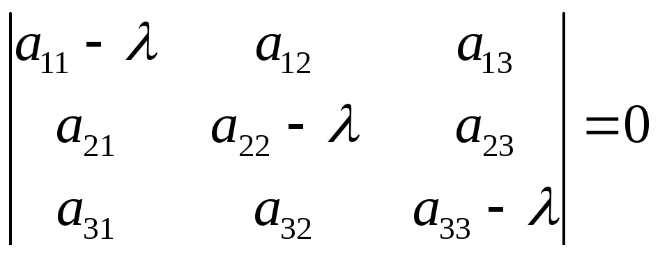
Поскольку нас интересуют только нетривиальные решения (xne o) однородной системы, то определитель матрицы системы должен быть равен нулю:

$det(A-lambda E)=begin{vmatrix}a_{11}-lambda&a_{12}&cdots&a_{1n}\ a_{21}&a_{22}-lambda&cdots&a_{2n}\ vdots&vdots&ddots&vdots\ a_{n1}&a_{n2}& cdots&a_{nn}-lambda end{vmatrix}=0.$

(7.15)

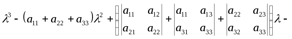
В противном случае по теореме 5.1 система имеет единственное тривиальное решение. Таким образом, задача нахождения собственных значений матрицы свелась к решению уравнения (7.15), т.е. к отысканию корней характеристического многочлена $Delta_{A}(lambda)=det(A-lambda E)$ матрицы . Уравнение $Delta_{A}(lambda)=0$ называется характеристическим уравнением матрицы . Так как характеристический многочлен имеет n-ю степень, то характеристическое уравнение — это алгебраическое уравнение n-го порядка. Согласно следствию 1 основной теоремы алгебры, характеристический многочлен можно представить в виде

$Delta_{A}(lambda)= det(A-lambda E)= a_{n}(lambda-lambda_1)^{n_1}cdot (lambda-lambda_2)^{n_2}cdotldotscdot(lambda-lambda_k)^{n_k},$

где lambda_1,lambda_2,ldots,lambda_k — корни многочлена кратности n_1,n_2,ldots,n_k соответственно, причем n_1+n_2+ldots+n_k=n . Другими словами, характеристический многочлен имеет п корней, если каждый корень считать столько раз, какова его кратность.

Теорема 7.4 о собственных значениях матрицы. Все корни характеристического многочлена (характеристического уравнения (7-15)) и только они являются собственными значениями матрицы.

Действительно, если число lambda — собственное значение матрицы , которому соответствует собственный вектор xne o , то однородная система (7.14) имеет нетривиальное решение, следовательно, матрица системы вырожденная, т.е. число lambda удовлетворяет характеристическому уравнению (7.15). Наоборот, если lambda — корень характеристического многочлена, то определитель (7.15) матрицы однородной системы (7.14) равен нулю, т.е. operatorname{rg}(A-lambda E)<n .В этом случае система имеет бесконечное множество решений, включая ненулевые решения. Поэтому найдется столбец xne o , удовлетворяющий условию (7.14). Значит, lambda — собственное значение матрицы .

Свойства собственных векторов

Пусть — квадратная матрица n-го порядка.

1. Собственные векторы, соответствующие различным собственным значениям, линейно независимы.

В самом деле, пусть s_1 и s_2 — собственные векторы, соответствующие собственным значениям lambda_1 и lambda_2 , причем lambda_1ne lambda_2 . Составим произвольную линейную комбинацию этих векторов и приравняем ее нулевому столбцу:

alpha_1cdot s_1+alpha_2cdot s_2=o.

(7.16)

Надо показать, что это равенство возможно только в тривиальном случае, когда alpha_1=alpha_2=0 . Действительно, умножая обе части на матрицу и подставляя As_1=lambda_1s_1 и As_2=lambda_2s_2 имеем

A(alpha_1s_1+alpha_2s_2)=oquad Leftrightarrowquad alpha_1As_1+ alpha_2As_2= oquad Leftrightarrowquad alpha_1 lambda_1s_1+alpha_2 lambda_2s_2=o.

Прибавляя к последнему равенству равенство (7.16), умноженное на (-lambda_2) , получаем

alpha_1cdotlambda_1cdot s_1-alpha_2cdotlambda_2cdot s_2=oquad Leftrightarrowquad alpha_1cdot(lambda_1-lambda_2)cdot s_1=o.

Так как s_1ne o и lambda_1ne lambda_2 , делаем вывод, что alpha_1=0 . Тогда из (7.16) следует, что и alpha_2=0 (поскольку s_2ne o ). Таким образом, собственные векторы s_1 и s_2 линейно независимы. Доказательство для любого конечного числа собственных векторов проводится по индукции.

2. Ненулевая линейная комбинация собственных векторов, соответствующих одному собственному значению, является собственным вектором, соответствующим тому же собственному значению.

Действительно, если собственному значению lambda соответствуют собственные векторы s_1,ldots,s_k , то из равенств S_i=lambda s_i, i=1,ldots,k , следует, что вектор s=alpha_1s_1+ldots+alpha_ks_k также собственный, поскольку:

As=A(alpha_1s_1+ldots+alpha_ks_k)= alpha_1lambda s_1+ldots+alpha_klambda s_k=lambda(alpha_1s_1+ldots+alpha_ks_k)=lambda s.

3. Пусть $(A-lambda E)^{+}$ — присоединенная матрица для характеристической матрицы . Если lambda_0 — собственное значение матрицы , то любой ненулевой столбец матрицы $(A-lambda E)^{+}$ является собственным вектором, соответствующим собственному значению .

В самом деле, применяя формулу (7.7) имеем $(A-lambda E)(A-lambda E)^{+}=Delta_k(lambda)cdot E$ . Подставляя корень lambda_0 , получаем $(A-lambda_0E)(A-lambda_0E)^{+}=O$ . Если — ненулевой столбец матрицы $(A-lambda_0E)^{+}$ , то (A-lambda_0E)s=oLeftrightarrow As=lambda_0s . Значит, — собственный вектор матрицы .

Замечания 7.5

1. По основной теореме алгебры характеристическое уравнение имеет п в общем случае комплексных корней (с учетом их кратностей). Поэтому собственные значения и собственные векторы имеются у любой квадратной матрицы. Причем собственные значения матрицы определяются однозначно (с учетом их кратности), а собственные векторы — неоднозначно.

2. Чтобы из множества собственных векторов выделить максимальную линейно независимую систему собственных векторов, нужно для всех раз личных собственных значений lambda_1,lambda_2, ldots,lambda_k записать одну за другой системы линейно независимых собственных векторов, в частности, одну за другой фундаментальные системы решений однородных систем

(A-lambda_1E)cdot x=o,quad (A-lambda_2E)cdot x=o,quad ldots,quad (A-lambda_kE)cdot x=o.

Полученная система собственных векторов будет линейно независимой в силу свойства 1 собственных векторов.

3. Совокупность всех собственных значений матрицы (с учетом их кратностей) называют ее спектром.

4. Спектр матрицы называется простым, если собственные значения матрицы попарно различные (все корни характеристического уравнения простые).

5. Для простого корня lambda=lambda_0 характеристического уравнения соответствующий собственный вектор можно найти, раскладывая определитель матрицы (A-lambda_0E) по одной из строк. Тогда ненулевой вектор, компоненты которого равны алгебраическим дополнениям элементов одной из строк матрицы , является собственным вектором.

Нахождение собственных векторов и собственных значений матрицы

Для нахождения собственных векторов и собственных значений квадратной матрицы n-го порядка надо выполнить следующие действия.

1. Составить характеристический многочлен матрицы Delta_A(lambda)=det(A-lambda E) .

2. Найти все различные корни lambda_1,lambda_2,ldots,lambda_k характеристического уравнения Delta_A(lambda)=0 (кратности n_1,n_2,ldots,n_k (n_1+n_2+ldots+n_k=n) корней определять не нужно).

3. Для корня lambda-lambda_1 найти фундаментальную систему $varphi_1,varphi_2,ldots,varphi_{n-r}$ решений однородной системы уравнений

(A-lambda_1E)cdot x=o , где $r=operatorname{rg}(A-lambda_1E)$

Для этого можно использовать либо алгоритм решения однородной системы, либо один из способов нахождения фундаментальной матрицы (см. пункт 3 замечаний 5.3, пункт 1 замечаний 5.5).

4. Записать линейно независимые собственные векторы матрицы , отвечающие собственному значению lambda_1:

$s_1=C_1varphi_1,quad s_2=C_2varphi_2,quad ldots,quad s_{n-r}=C_{n-r}varphi_{n-r},$

(7.17)

где $C_1,C_2,ldots,C_{n-r}$ — отличные от нуля произвольные постоянные. Совокупность всех собственных векторов, отвечающих собственному значению lambda_1 , образуют ненулевые столбцы вида $s=C_1varphi_1+C_2varphi_2+ldots+C_{n-r}varphi_{n-r}$ . Здесь и далее собственные векторы матрицы будем обозначать буквой .

Повторить пункты 3,4 для остальных собственных значений lambda_1,lambda_2,ldots,lambda_k .

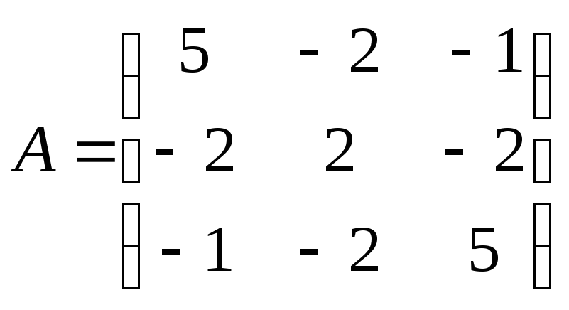
Пример 7.8. Найти собственные значения и собственные векторы матриц:

$A=begin{pmatrix}1&-2\3&8end{pmatrix}!,quad B=begin{pmatrix}1&-4\ 1&1 end{pmatrix}!,quad C=begin{pmatrix}1&1&1\1&1&1\1&1&1end{pmatrix}!.$

Решение. Матрица . 1. Составляем характеристический многочлен матрицы

$Delta_{A}(lambda)=begin{vmatrix}1-lambda&-2\3&8-lambdaend{vmatrix}= (1-lambda)(8-lambda)+6=lambda^2-9 lambda+8+6= lambda^2-9 lambda+14.$

2. Решаем характеристическое уравнение: $lambda^2-9 lambda+14=0~Rightarrow~! left[!begin{gathered}lambda_1=2,\ lambda_2=7.end{gathered}right.$ .

3(1). Для корня lambda_1=2 составляем однородную систему уравнений (A-lambda_1E)x=o:

$begin{pmatrix}1-2&-2\ 3&8-2 end{pmatrix}!cdot! begin{pmatrix}x_1\x_2 end{pmatrix}= begin{pmatrix}0\0end{pmatrix}quad Leftrightarrowquad begin{pmatrix}-1&-2\ 3&6 end{pmatrix}!cdot! begin{pmatrix}x_1\x_2 end{pmatrix}= begin{pmatrix}0\0 end{pmatrix}!.$

Решаем эту систему методом Гаусса, приводя расширенную матрицу системы к упрощенному виду

$begin{pmatrix}-1&-2!!&vline!!&0\ 3&6!!&vline!!&0end{pmatrix}sim begin{pmatrix}1&2!!&vline!!&0\ 3&6!!&vline!!&0end{pmatrix}sim begin{pmatrix}1&2!!& vline!!&0\ 0&0!!&vline!!&0end{pmatrix}!.$

Ранг матрицы системы равен 1 (r=1) , число неизвестных n=2 , следовательно, фундаментальная система решений состоит из n-r=1 решения. Выражаем базисную переменную x_1 через свободную: x_1=-2x_2 . Полагая x_2=1 , получаем решение $varphi_1= begin{pmatrix}-2\1end{pmatrix}$ .

4(1). Записываем собственные векторы, соответствующие собственному значению lambda_1=2colon~ s_1=C_1cdotvarphi_1 , где C_1 — отличная от нуля произвольная постоянная.

Заметим, что, согласно пункту 5 замечаний 7.5, в качестве собственного вектора можно выбрать вектор, составленный из алгебраических дополнений элементов второй строки матрицы $begin{pmatrix}-1&-2\3&6end{pmatrix}$ , то есть $begin{pmatrix}2\-1 end{pmatrix}$ . Умножив этот столбец на (-1), получим varphi_1 .

3(2). Для корня lambda_2=7 составляем однородную систему уравнений (A-lambda_2E)x=o:

$begin{pmatrix}1-7&-2\ 3&8-7 end{pmatrix}!cdot! begin{pmatrix}x_1\x_2 end{pmatrix}= begin{pmatrix}0\0end{pmatrix}quad Leftrightarrowquad begin{pmatrix}-6&-2\ 3&1 end{pmatrix}!cdot! begin{pmatrix}x_1\x_2 end{pmatrix}= begin{pmatrix}0\0 end{pmatrix}!.$

Решаем эту систему методом Гаусса, приводя расширенную матрицу системы к упрощенному виду

$begin{pmatrix}-6&-2!!&vline!!&0\ 3&1!!&vline!!&0end{pmatrix}sim begin{pmatrix}3&1!!&vline!!&0\ -6&-2!!&vline!!&0end{pmatrix}sim begin{pmatrix}1&1/3!!& vline!!&0\ -6&-2!!&vline!!&0end{pmatrix}sim begin{pmatrix}1&1/3!!& vline!!&0\ 0&0!!&vline!!&0end{pmatrix}!.$

Ранг матрицы системы равен 1 (r=1) , число неизвестных n=2 , следовательно, фундаментальная система решений состоит из n-r=1 решения. Выражаем базисную переменную x_1 через свободную: $x_1=-frac{1}{3}x_2$ . Полагая x_2=1 , получаем решение $varphi_2=begin{pmatrix}-1/3\1end{pmatrix}$ .

4(2). Записываем собственные векторы, соответствующие собственному значению lambda_2=7colon~ s_2=C_2cdotvarphi_2 , где C_2 — отличная от нуля произвольная постоянная.

Заметим, что, согласно пункту 5 замечаний 7.5, в качестве собственного вектора можно выбрать вектор, составленный из алгебраических дополнений элементов первой строки матрицы $begin{pmatrix}-6&-2\3&1end{pmatrix}$ , т.е. $begin{pmatrix}1\-3 end{pmatrix}$ . Поделив его на (- 3), получим varphi_2 .

Матрица . 1. Составляем характеристический многочлен матрицы

$Delta_{B}(lambda)= begin{vmatrix}1-lambda&-4\1&1-lambdaend{vmatrix}= (1-lambda)^2+4=lambda^2-2 lambda+1+4= lambda^2-2 lambda+5.$

2. Решаем характеристическое уравнение: $lambda^2-2 lambda+5=0~Rightarrow~! left[! begin{gathered}lambda_1=1+2i,\ lambda_2=1-2i.end{gathered}right.$ .

3(1). Для корня lambda_1=1+2i составляем однородную систему уравнений (B-lambda_1E)x=o

$begin{pmatrix}1-(1+2i)&-4\ 1&8-1-(1+2i) end{pmatrix}!cdot! begin{pmatrix}x_1\x_2 end{pmatrix}= begin{pmatrix}0\0end{pmatrix}quad Leftrightarrowquad begin{pmatrix}-2i&-4\ 1&-2i end{pmatrix}!cdot! begin{pmatrix}x_1\x_2 end{pmatrix}= begin{pmatrix}0\0 end{pmatrix}!.$

Решаем эту систему методом Гаусса, приводя расширенную матрицу системы к упрощенному виду

$begin{pmatrix}-2i&-4!!&vline!!&0\ 1&-2i!!&vline!!&0end{pmatrix}sim begin{pmatrix} 1&-2i!!&vline!!&0\ -2i&-4!!&vline!!&0end{pmatrix}sim begin{pmatrix}1&-2i!!& vline!!&0\ 0&0!!&vline!!&0end{pmatrix}.$

Ранг матрицы системы равен 1 (r=1) , число неизвестных n=2 , следовательно, фундаментальная система решений состоит из n-r=1 решения. Выражаем базисную переменную x_1 через свободную: x_1=2i,x_2 . Полагая x_2=1 , получаем решение $varphi_1= begin{pmatrix}2i\1 end{pmatrix}$ .

4(1). Записываем собственные векторы, соответствующие собственному значению lambda_1= 1+2icolon~ s_1=C_1cdotvarphi_1 , где C_1 — отличная от нуля произвольная постоянная.

Заметим, что, согласно пункту 5 замечаний 7.5, в качестве собственного вектора можно выбрать вектор, составленный из алгебраических дополнений элементов первой строки матрицы $begin{pmatrix}-2i&-4\1&-2iend{pmatrix}$ , то есть $begin{pmatrix}-2i\ -1 end{pmatrix}$ . Умножив этот столбец на (-1), получим varphi_1 .

3(2). Для корня lambda_2=1-2i составляем однородную систему уравнений (B-lambda_2E)x=o:

$begin{pmatrix}1-(1-2i)&-4\ 1&8-1-(1-2i) end{pmatrix}!cdot! begin{pmatrix}x_1\x_2 end{pmatrix}= begin{pmatrix}0\0end{pmatrix}quad Leftrightarrowquad begin{pmatrix}2i&-4\ 1&2i end{pmatrix}!cdot! begin{pmatrix}x_1\x_2 end{pmatrix}= begin{pmatrix}0\0 end{pmatrix}!.$

Решаем эту систему методом Гаусса, приводя расширенную матрицу системы к упрощенному виду

$begin{pmatrix}2i&-4!!&vline!!&0\ 1&2i!!&vline!!&0end{pmatrix}sim begin{pmatrix} 1&2i!!&vline!!&0\ 2i&-4!!&vline!!&0end{pmatrix}sim begin{pmatrix}1&2i!!& vline!!&0\ 0&0!!&vline!!&0end{pmatrix}.$

Ранг матрицы системы равен 1 (r=1) , число неизвестных n=2 , следовательно, фундаментальная система решений состоит из n-r=1 решения. Выражаем базисную переменную x_1 через свободную: x_1=-2i,x_2 . Полагая x_2=1 , получаем решение $varphi_2= begin{pmatrix}-2i\1 end{pmatrix}$ .

4(2). Записываем собственные векторы, соответствующие собственному значению lambda_2=1-2icolon~ s_2=C_2cdotvarphi_2 , где C_2 — отличная от нуля произвольная постоянная.

Заметим, что, согласно пункту 5 замечаний 7.5, в качестве собственного вектора можно выбрать вектор, составленный из алгебраических дополнений элементов первой строки матрицы $begin{pmatrix}2i&-4\1&2iend{pmatrix}$ , т.е. $begin{pmatrix}2i\-1 end{pmatrix}$ . Умножив его на (-1), получим varphi_2 .

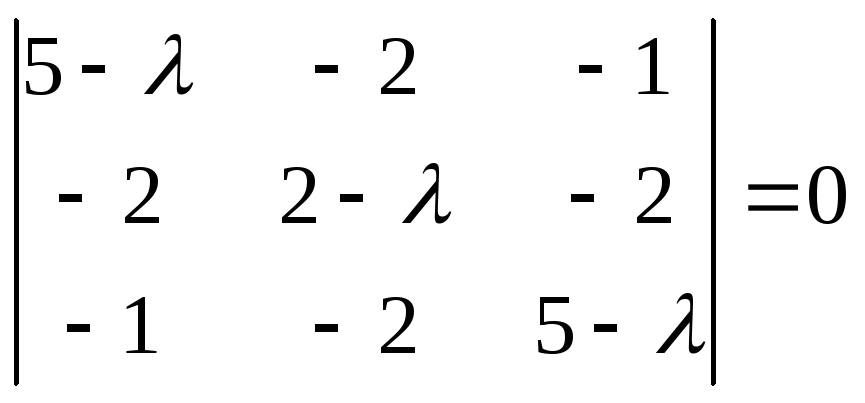
Матрица 1. Составляем характеристический многочлен матрицы

$Delta_{C}(lambda)= det(C-lambda E)= begin{vmatrix}1-lambda&1&1\1&1-lambda&1\ 1&1&1-lambda end{vmatrix}= (1-lambda)^3+2-3(1-lambda)= -lambda^3+3 lambda^2.$

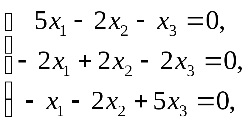
2. Решаем характеристическое уравнение: $-lambda^3+3 lambda^2=0~Rightarrow~! left[! begin{gathered}lambda_1=3,\ lambda_2=0end{gathered}right.$ .

3(1). Для корня lambda_1=3 составляем однородную систему уравнений (C-lambda_1E)x=o:

$begin{pmatrix}1-3&1&1\ 1&1-3&1\ 1&1&1-3end{pmatrix}!cdot! begin{pmatrix} x_1\x_2\x_3end{pmatrix}=begin{pmatrix}0\0\0end{pmatrix}quad Leftrightarrowquad begin{cases}-2x_1+x_2+x_3=0,\ x_1-2x_2+x_3=0,\ x_1+x_2-2x_3=0.end{cases}$

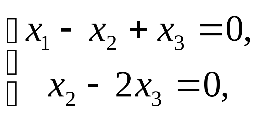
Решаем эту систему методом Гаусса, приводя расширенную матрицу системы к упрощенному виду (ведущие элементы выделены полужирным курсивом):

$begin{gathered}begin{pmatrix}C-lambda_1Emid oend{pmatrix}= begin{pmatrix} -2&1&1!!&vline!!&0\ 1&-2&1!!&vline!!&0\ 1&1&-2!!&vline!!&0 end{pmatrix}sim begin{pmatrix} 1&1&-2!!&vline!!&0\ -2&1&1!!&vline!!&0\ 1&-2&1!!&vline!!&0 end{pmatrix}sim\[2pt] simbegin{pmatrix} 1&1&-2!!&vline!!&0\ 0&3&-3!!&vline!!&0\ 0&-3&3!!&vline!!&0 end{pmatrix}sim begin{pmatrix} 1&1&-2!!&vline!!&0\ 0&1&-1!!&vline!!&0\ 0&0&0!!&vline!!&0 end{pmatrix}sim begin{pmatrix} 1&0&-1!!&vline!!&0\ 0&1&-1!!&vline!!&0\ 0&0&0!!&vline!!&0 end{pmatrix}!.end{gathered}$

Ранг матрицы системы равен 2 (r=2) , число неизвестных n=3 , следовательно, фундаментальная система решений состоит из n-r=1 решения. Выражаем базисные переменные x_1,x_2 через свободную $x_3colon begin{cases}x_1=x_3,\x_2=x_3,end{cases}$ и, полагая x_3=1 , получаем решение $varphi=begin{pmatrix}1\1\1end{pmatrix}$ .

4(1). Все собственные векторы, соответствующие собственному значению lambda_1=3 , вычисляются по формуле s=C_1cdotvarphi , где C_1 — отличная от нуля произвольная постоянная.

Заметим, что, согласно пункту 5 замечаний 7.5, в качестве собственного вектора можно выбрать вектор, составленный из алгебраических дополнений элементов первой строки матрицы $begin{pmatrix}-2&1&1\1&-2&1\1&1&-2end{pmatrix}$ , то есть $begin{pmatrix}3\3\3end{pmatrix}$ , так как

$A_{11}=(-1)^{1+1}begin{vmatrix} -2&1\1&-2 end{vmatrix} =3;quad A_{12}=(-1)^{1+2} begin{vmatrix} 1&1\1&-2 end{vmatrix}= 3;quad A_{13}=(-1)^{1+3}begin{vmatrix}1&-2\ 1&1 end{vmatrix}=3.$

Разделив его на 3, получим varphi .

3(2). Для собственного значения lambda_2=0 имеем однородную систему Cx=o . Решаем ее методом Гаусса:

$begin{pmatrix}Cmid oend{pmatrix}= begin{pmatrix}1&1&1!!&vline!!&0\ 1&1&1!!&vline!!&0\ 1&1&1!!&vline!!&0 end{pmatrix}sim begin{pmatrix}1&1&1!!& vline!!&0\ 0&0&0!!&vline!!&0\ 0&0&0!!&vline!!&0 end{pmatrix}!.$

Ранг матрицы системы равен единице (r=1) , следовательно, фундаментальная система решений состоит из двух решений (n-r=2) . Базисную переменную x_1 , выражаем через свободные: x_1=-x_2-x_3 . Задавая стандартные наборы свободных переменных x_2=1,~x_3=0 и x_2=0,~ x_3=1 , получаем два решения

$varphi_1=begin{pmatrix}-1\1\0end{pmatrix}!,qquad varphi_2=begin{pmatrix}-1\0\1 end{pmatrix}!.$

4(2). Записываем множество собственных векторов, соответствующих собственному значению lambda_2=0colon~ s=C_1varphi_1+C_2varphi_2 , где C_1,C_2 — произвольные постоянные, не равные нулю одновременно. В частности, при C_1=0, C_2=-1 получаем $s_1=begin{pmatrix}1&0&-1end{pmatrix}^T$ ; при C_1=0,~C_2=-1colon $s_2=begin{pmatrix}1&-1&0end{pmatrix}^T$ . Присоединяя к этим собственным векторам собственный вектор $s_3=begin{pmatrix}1&1&1 end{pmatrix}^T$ , соответствующий собственному значению lambda_1=3 (см. пункт 4(1) при C_1=1 ), находим три линейно независимых собственных вектора матрицы

$s_1=begin{pmatrix}1\0\-1end{pmatrix}!,qquad s_2=begin{pmatrix}1\-1\0 end{pmatrix}!,qquad s_3=begin{pmatrix}1\1\1end{pmatrix}!.$

Заметим, что для корня lambda_2=0 собственный вектор нельзя найти, применяя пункт 5 замечаний 7.5, так как алгебраическое дополнение каждого элемента матрицы равно нулю.

Математический форум (помощь с решением задач, обсуждение вопросов по математике).

Кнопка "Поделиться"

Если заметили ошибку, опечатку или есть предложения, напишите в комментариях.

Источник

В этой главе
рассматриваются вопросы о собственных
векторах и собственных значениях
произвольной квадратной матрицы,
симметрической матрицы и подобных
матриц.

1. Основные понятия.

Определение.
Вектор
,
называетсясобственным
вектором
квадратной матрицы
,
если существует такое число,
что

.
При
этом числоназываетсясобственным
значением
матрицы
,
соответствующим собственному вектору.

Уравнение
может быть записано в виде

Определение.
Если
— собственное значение матрицы,
асоответствующий ему собственный вектор,
тоназываютсобственной
парой матрицы
.

● Пример 1.
Показать,
что вектор
является собственным вектором матрицы.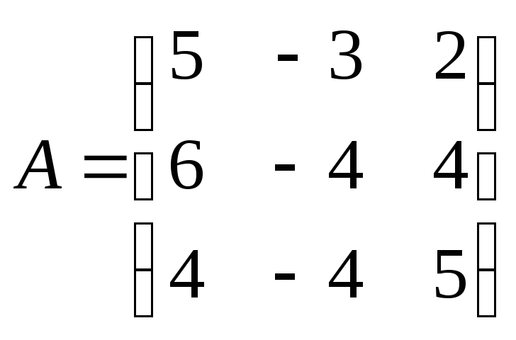
Найти
соответствующее ему собственное
значение.

Решение.

Так как
(),
то—
собственный вектор матрицы,
соответствующий собственному значению.●

● Пример 2.
Показать,
что если
— собственная пара матрицы,
то— собственная пара матрицы.

Решение.
Действительно,

,
т.е.
.
Из последнего следует, что— собственная пара матрицы.●

● Пример 3.
При каких
ивекторявляется собственным вектором матрицы?

Решение.
Найдем вектор
..

Если —
собственный вектор матрицы
,
то,
откуда.
Из последнего имеемии.

Ответ:
при
и произвольномвекторсобственный вектор матрицы.

● Пример 4.
Существует
ли
,
при котором—
собственный вектор матрицы?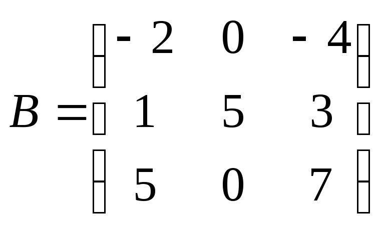
Если существует, указать соответствующую
собственную пару.

Решение.
Вычислим произведение

Если
—
собственная пара матрицы,
то

Из последнего
равенства имеем
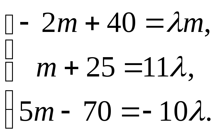Откуда,,.

—
собственная пара матрицы.●

2. Свойства собственных векторов.

1)
Если —
собственный вектор матрицы
,
а—
соответствующее ему собственное
значение, то при любомвектортакже является собственным вектором
этой матрицы, соответствующим этому же
собственному значению.

►Действительно,
.◄

Замечание. Любой
собственный вектор матрицы определяет
целое направление
собственных векторов этой матрицы с
одним и тем же собственным значением.

2)
Собственные векторы матрицы, соответствующие
различным
её собственным значениям, линейно
независимы.

►Доказательство.
Пусть
и—
собственные пары матрицы,
где.

Предположим, что
илинейно зависимые векторы.

Если
илинейно зависимы, то хотя бы один из
этих векторов можно представить в виде
линейной комбинации другого (пусть).

Тогда
,
откуда следует, что.
Так как,
то.

Полученное
противоречие доказывает утверждение.◄

3)
Если
илинейно независимые собственные векторы
матрицы,
соответствующие одному и тому же
собственному значению,
то любая нетривиальная линейная
комбинация этих векторов()
также является собственным вектором
этой матрицы, соответствующим этому же
собственному значению.

►Действительно,
,

что и требовалось доказать.◄

4)
Если матрица
диагональная
,
то ее собственные значения совпадают
с диагональными элементами этой матрицы
(),
а единичный векторявляется собственным вектором,
соответствующим собственному значению.

►Действительно,
◄

3 Нахождение собственных значений и собственных векторов.

Собственные
значения и собственные векторы матрицы
удовлетворяют матричному уравнению.

Если
собственный вектор матрицы
,
то однородная системаимеет нетривиальное решение, поэтому(порядок
матрицыи.
Последнее
уравнение позволяет найти собственные
значения матрицы.

Определение.
Многочлен
называютхарактеристическим многочленомматрицы.

Определение.
Уравнение

называется
характеристическим
уравнением
матрицы
.

Корни характеристического
уравнения
матрицы
являются собственными значениями
матрицы.

Характеристическое
уравнение матрицы
может быть записано в виде.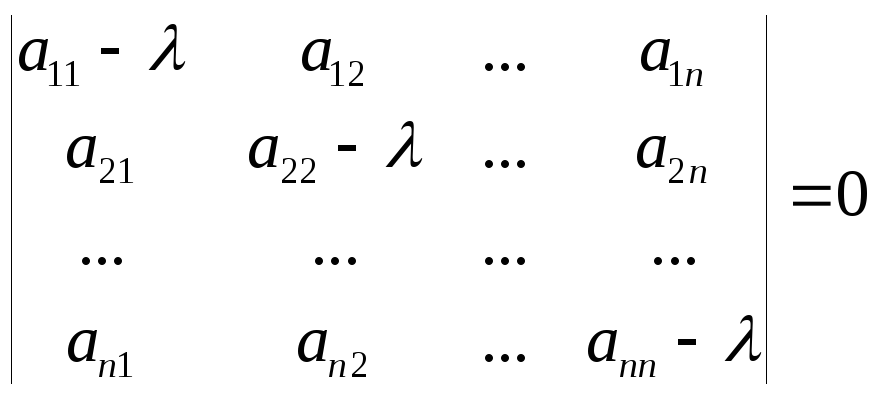

Определение.
Множество всех собственных значений
квадратной матрицы называется спектром
этой
матрицы.

Спектр матрицы
-го
порядка содержитсобственных значений матрицы, которые
могут быть как действительными, так и
комплексными, простыми так и кратными.

Для матрицы
характеристическое уравнениеможет быть может быть преобразовано к
виду
.

,
поэтому характеристическое уравнение
матрицы
имеет вид

. (8.1)

При этом

,(8.2)

.(8.3)

Уравнение
является характеристическим уравнением
матрицы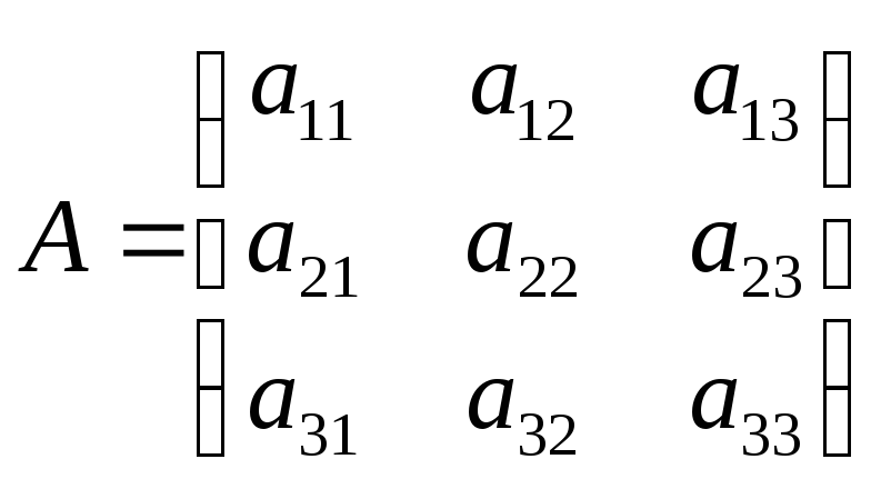.Это
уравнение может быть представлено в
виде

или

,
(8.4)

где
,
аминоры определителя.

Если
,икорни характеристического уравнения
(8.4), то это уравнение может быть записано
в виде

. (8.5)

Сравнивая уравнения
(8.4) и (8.5), можно записать следующее:

,(8.6)

,(8.7)

.(8.8)

Собственные векторы
матрицы
,
соответствующие собственному значению,
удовлетворяют матричному уравнению,
которое может быть записана в форме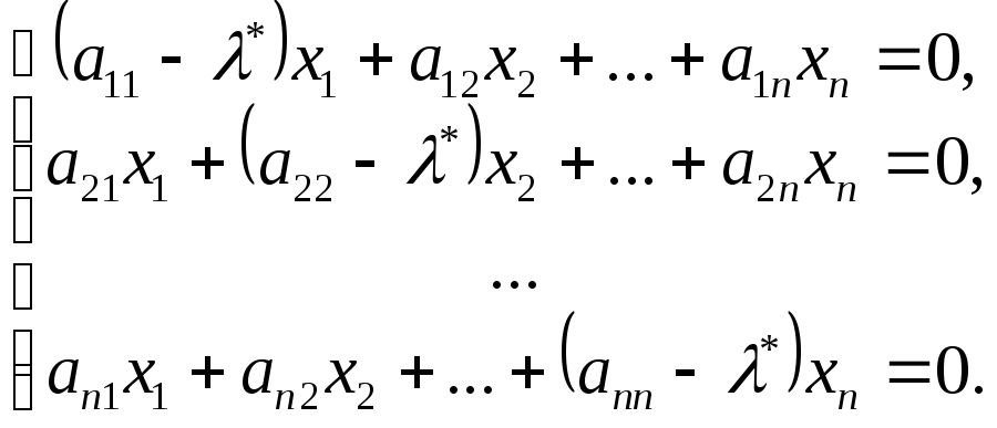Так
как ранг матрицы этой системы меньше
числа неизвестных (=0),
то система имеет бесконечное множество

решений, каждое
ненулевое
из которых является собственным вектором,
соответствующим собственному значению
.

● Пример 5.
Найти собственные значения и собственные
векторы матрицы
.

Решение.
— характеристическое уравнение для
данной матрицы, откуда,и.

Для нахождения
собственных векторов, соответствующих
собственному
значению
,
имеем системуэквивалентную уравнению.
Векторявляется решением этого уравнения, а
привектор— искомый собственный вектор.

Для
нахождения собственных векторов,
соответствующих собственному значению
,
имеем системуиз которой следует, что векторприявляется собственным вектором,
соответствующим собственному значению.

Ответ.
,при;,при.

● Пример 6.

Найти собственные
пары матрицы
.

Решение.
— характеристическоеуравнение
матрицы
,
которое может быть записано в виде,
где,,,,(проверьте).

—
характеристическое уравнение матрицы
,
корни которого.

Собственные
векторы, соответствующие собственному
значению
,
находим из системы.
Приимеем систему
которая
равносильна системе
решение
которой
.

При
векторявляется собственным вектором матрицы,
соответствующим собственному значению.

При
для нахождения собственных векторов
имеем системукоторая равносильна одному уравнению.

При любых
ивекторесть решение уравнения,
а при

является собственным
вектором, который соответствует
собственному значению
.

Ответ:
при;при.

● Пример 7.
Найти собственные значения и собственные
векторы матрицы
.

Решение.
Характеристическое уравнение для
указанной матрицы имеет вид
,
откудаи.

Для нахождения
собственных векторов, соответствующих
собственному значению
,
имеем системуиз которой следуетпри.

Ответ.
,при;,при.

● Пример 8.

Доказать, что если
собственная
пара невырожденной матрицы
,
то
—собственная
пара матрицы
.

►Так матрица
невырожденная (),
то существует.
Произведение собственных значений
матрицыравно,
а так как,
то собственное значение.

— собственная
пара матрицы
,
поэтому.Умножив
последнее равенство слева на
,
имеем,
откуда,и.
Последнее равенство означает, что
—
собственная
пара матрицы
.◄

Соседние файлы в предмете [НЕСОРТИРОВАННОЕ]

Источник

In linear algebra, an eigenvector () or characteristic vector of a linear transformation is a nonzero vector that changes at most by a scalar factor when that linear transformation is applied to it. The corresponding eigenvalue, often denoted by lambda , is the factor by which the eigenvector is scaled.

Geometrically, an eigenvector, corresponding to a real nonzero eigenvalue, points in a direction in which it is stretched by the transformation and the eigenvalue is the factor by which it is stretched. If the eigenvalue is negative, the direction is reversed.^[1] Loosely speaking, in a multidimensional vector space, the eigenvector is not rotated.

Formal definition[edit]

If T is a linear transformation from a vector space V over a field F into itself and v is a nonzero vector in V, then v is an eigenvector of T if T(v) is a scalar multiple of v.^[2] This can be written as

where λ is a scalar in F, known as the eigenvalue, characteristic value, or characteristic root associated with v.

There is a direct correspondence between n-by-n square matrices and linear transformations from an n-dimensional vector space into itself, given any basis of the vector space. Hence, in a finite-dimensional vector space, it is equivalent to define eigenvalues and eigenvectors using either the language of matrices, or the language of linear transformations.^[3]^[4]

If V is finite-dimensional, the above equation is equivalent to^[5]

where A is the matrix representation of T and u is the coordinate vector of v.

Overview[edit]

Eigenvalues and eigenvectors feature prominently in the analysis of linear transformations. The prefix eigen- is adopted from the German word eigen (cognate with the English word own) for ‘proper’, ‘characteristic’, ‘own’.^[6]^[7] Originally used to study principal axes of the rotational motion of rigid bodies, eigenvalues and eigenvectors have a wide range of applications, for example in stability analysis, vibration analysis, atomic orbitals, facial recognition, and matrix diagonalization.

In essence, an eigenvector v of a linear transformation T is a nonzero vector that, when T is applied to it, does not change direction. Applying T to the eigenvector only scales the eigenvector by the scalar value λ, called an eigenvalue. This condition can be written as the equation

referred to as the eigenvalue equation or eigenequation. In general, λ may be any scalar. For example, λ may be negative, in which case the eigenvector reverses direction as part of the scaling, or it may be zero or complex.

In this shear mapping the red arrow changes direction, but the blue arrow does not. The blue arrow is an eigenvector of this shear mapping because it does not change direction, and since its length is unchanged, its eigenvalue is 1.

A 2×2 real and symmetric matrix representing a stretching and shearing of the plane. The eigenvectors of the matrix (red lines) are the two special directions such that every point on them will just slide on them.

The Mona Lisa example pictured here provides a simple illustration. Each point on the painting can be represented as a vector pointing from the center of the painting to that point. The linear transformation in this example is called a shear mapping. Points in the top half are moved to the right, and points in the bottom half are moved to the left, proportional to how far they are from the horizontal axis that goes through the middle of the painting. The vectors pointing to each point in the original image are therefore tilted right or left, and made longer or shorter by the transformation. Points along the horizontal axis do not move at all when this transformation is applied. Therefore, any vector that points directly to the right or left with no vertical component is an eigenvector of this transformation, because the mapping does not change its direction. Moreover, these eigenvectors all have an eigenvalue equal to one, because the mapping does not change their length either.

Linear transformations can take many different forms, mapping vectors in a variety of vector spaces, so the eigenvectors can also take many forms. For example, the linear transformation could be a differential operator like ${tfrac {d}{dx}}$ , in which case the eigenvectors are functions called eigenfunctions that are scaled by that differential operator, such as

${displaystyle {frac {d}{dx}}e^{lambda x}=lambda e^{lambda x}.}$

Alternatively, the linear transformation could take the form of an n by n matrix, in which case the eigenvectors are n by 1 matrices. If the linear transformation is expressed in the form of an n by n matrix A, then the eigenvalue equation for a linear transformation above can be rewritten as the matrix multiplication

where the eigenvector v is an n by 1 matrix. For a matrix, eigenvalues and eigenvectors can be used to decompose the matrix—for example by diagonalizing it.

Eigenvalues and eigenvectors give rise to many closely related mathematical concepts, and the prefix eigen- is applied liberally when naming them:

The set of all eigenvectors of a linear transformation, each paired with its corresponding eigenvalue, is called the eigensystem of that transformation.^[8]^[9]
The set of all eigenvectors of T corresponding to the same eigenvalue, together with the zero vector, is called an eigenspace, or the characteristic space of T associated with that eigenvalue.^[10]
If a set of eigenvectors of T forms a basis of the domain of T, then this basis is called an eigenbasis.

History[edit]

Eigenvalues are often introduced in the context of linear algebra or matrix theory. Historically, however, they arose in the study of quadratic forms and differential equations.

In the 18th century, Leonhard Euler studied the rotational motion of a rigid body, and discovered the importance of the principal axes.^[a] Joseph-Louis Lagrange realized that the principal axes are the eigenvectors of the inertia matrix.^[11]

In the early 19th century, Augustin-Louis Cauchy saw how their work could be used to classify the quadric surfaces, and generalized it to arbitrary dimensions.^[12] Cauchy also coined the term racine caractéristique (characteristic root), for what is now called eigenvalue; his term survives in characteristic equation.^[b]

Later, Joseph Fourier used the work of Lagrange and Pierre-Simon Laplace to solve the heat equation by separation of variables in his famous 1822 book Théorie analytique de la chaleur.^[13] Charles-François Sturm developed Fourier’s ideas further, and brought them to the attention of Cauchy, who combined them with his own ideas and arrived at the fact that real symmetric matrices have real eigenvalues.^[12] This was extended by Charles Hermite in 1855 to what are now called Hermitian matrices.^[14]

Around the same time, Francesco Brioschi proved that the eigenvalues of orthogonal matrices lie on the unit circle,^[12] and Alfred Clebsch found the corresponding result for skew-symmetric matrices.^[14] Finally, Karl Weierstrass clarified an important aspect in the stability theory started by Laplace, by realizing that defective matrices can cause instability.^[12]

In the meantime, Joseph Liouville studied eigenvalue problems similar to those of Sturm; the discipline that grew out of their work is now called Sturm–Liouville theory.^[15] Schwarz studied the first eigenvalue of Laplace’s equation on general domains towards the end of the 19th century, while Poincaré studied Poisson’s equation a few years later.^[16]

At the start of the 20th century, David Hilbert studied the eigenvalues of integral operators by viewing the operators as infinite matrices.^[17] He was the first to use the German word eigen, which means «own»,^[7] to denote eigenvalues and eigenvectors in 1904,^[c] though he may have been following a related usage by Hermann von Helmholtz. For some time, the standard term in English was «proper value», but the more distinctive term «eigenvalue» is the standard today.^[18]

The first numerical algorithm for computing eigenvalues and eigenvectors appeared in 1929, when Richard von Mises published the power method. One of the most popular methods today, the QR algorithm, was proposed independently by John G. F. Francis^[19] and Vera Kublanovskaya^[20] in 1961.^[21]^[22]

Eigenvalues and eigenvectors of matrices[edit]

Eigenvalues and eigenvectors are often introduced to students in the context of linear algebra courses focused on matrices.^[23]^[24]
Furthermore, linear transformations over a finite-dimensional vector space can be represented using matrices,^[3]^[4] which is especially common in numerical and computational applications.^[25]

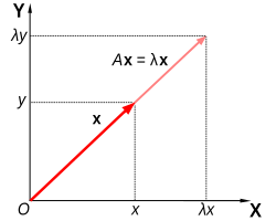
Matrix A acts by stretching the vector x, not changing its direction, so x is an eigenvector of A.

Consider n-dimensional vectors that are formed as a list of n scalars, such as the three-dimensional vectors

${displaystyle mathbf {x} ={begin{bmatrix}1\-3\4end{bmatrix}}quad {mbox{and}}quad mathbf {y} ={begin{bmatrix}-20\60\-80end{bmatrix}}.}$

These vectors are said to be scalar multiples of each other, or parallel or collinear, if there is a scalar λ such that

In this case ${displaystyle lambda =-{frac {1}{20}}}$ .

Now consider the linear transformation of n-dimensional vectors defined by an n by n matrix A,

${displaystyle {begin{bmatrix}A_{11}&A_{12}&cdots &A_{1n}\A_{21}&A_{22}&cdots &A_{2n}\vdots &vdots &ddots &vdots \A_{n1}&A_{n2}&cdots &A_{nn}\end{bmatrix}}{begin{bmatrix}v_{1}\v_{2}\vdots \v_{n}end{bmatrix}}={begin{bmatrix}w_{1}\w_{2}\vdots \w_{n}end{bmatrix}}}$

where, for each row,

${displaystyle w_{i}=A_{i1}v_{1}+A_{i2}v_{2}+cdots +A_{in}v_{n}=sum _{j=1}^{n}A_{ij}v_{j}.}$

If it occurs that v and w are scalar multiples, that is if

(1)

then v is an eigenvector of the linear transformation A and the scale factor λ is the eigenvalue corresponding to that eigenvector. Equation (1) is the eigenvalue equation for the matrix A.

Equation (1) can be stated equivalently as

(2)

where I is the n by n identity matrix and 0 is the zero vector.

Eigenvalues and the characteristic polynomial[edit]

Equation (2) has a nonzero solution v if and only if the determinant of the matrix (A − λI) is zero. Therefore, the eigenvalues of A are values of λ that satisfy the equation

(3)

Using the Leibniz formula for determinants, the left-hand side of Equation (3) is a polynomial function of the variable λ and the degree of this polynomial is n, the order of the matrix A. Its coefficients depend on the entries of A, except that its term of degree n is always (−1)ⁿλⁿ. This polynomial is called the characteristic polynomial of A. Equation (3) is called the characteristic equation or the secular equation of A.

The fundamental theorem of algebra implies that the characteristic polynomial of an n-by-n matrix A, being a polynomial of degree n, can be factored into the product of n linear terms,

${displaystyle |A-lambda I|=(lambda _{1}-lambda )(lambda _{2}-lambda )cdots (lambda _{n}-lambda ),}$

(4)

where each λ_i may be real but in general is a complex number. The numbers λ₁, λ₂, …, λ_n, which may not all have distinct values, are roots of the polynomial and are the eigenvalues of A.

As a brief example, which is described in more detail in the examples section later, consider the matrix

${displaystyle A={begin{bmatrix}2&1\1&2end{bmatrix}}.}$

Taking the determinant of (A − λI), the characteristic polynomial of A is

${displaystyle |A-lambda I|={begin{vmatrix}2-lambda &1\1&2-lambda end{vmatrix}}=3-4lambda +lambda ^{2}.}$

Setting the characteristic polynomial equal to zero, it has roots at λ=1 and λ=3, which are the two eigenvalues of A. The eigenvectors corresponding to each eigenvalue can be found by solving for the components of v in the equation . In this example, the eigenvectors are any nonzero scalar multiples of

${displaystyle mathbf {v} _{lambda =1}={begin{bmatrix}1\-1end{bmatrix}},quad mathbf {v} _{lambda =3}={begin{bmatrix}1\1end{bmatrix}}.}$

If the entries of the matrix A are all real numbers, then the coefficients of the characteristic polynomial will also be real numbers, but the eigenvalues may still have nonzero imaginary parts. The entries of the corresponding eigenvectors therefore may also have nonzero imaginary parts. Similarly, the eigenvalues may be irrational numbers even if all the entries of A are rational numbers or even if they are all integers. However, if the entries of A are all algebraic numbers, which include the rationals, the eigenvalues must also be algebraic numbers (that is, they cannot magically become transcendental numbers).

The non-real roots of a real polynomial with real coefficients can be grouped into pairs of complex conjugates, namely with the two members of each pair having imaginary parts that differ only in sign and the same real part. If the degree is odd, then by the intermediate value theorem at least one of the roots is real. Therefore, any real matrix with odd order has at least one real eigenvalue, whereas a real matrix with even order may not have any real eigenvalues. The eigenvectors associated with these complex eigenvalues are also complex and also appear in complex conjugate pairs.

Algebraic multiplicity[edit]

Let λ_i be an eigenvalue of an n by n matrix A. The algebraic multiplicity μ_A(λ_i) of the eigenvalue is its multiplicity as a root of the characteristic polynomial, that is, the largest integer k such that (λ − λ_i)^k divides evenly that polynomial.^[10]^[26]^[27]

Suppose a matrix A has dimension n and d ≤ n distinct eigenvalues. Whereas Equation (4) factors the characteristic polynomial of A into the product of n linear terms with some terms potentially repeating, the characteristic polynomial can instead be written as the product of d terms each corresponding to a distinct eigenvalue and raised to the power of the algebraic multiplicity,

${displaystyle |A-lambda I|=(lambda _{1}-lambda )^{mu _{A}(lambda _{1})}(lambda _{2}-lambda )^{mu _{A}(lambda _{2})}cdots (lambda _{d}-lambda )^{mu _{A}(lambda _{d})}.}$

If d = n then the right-hand side is the product of n linear terms and this is the same as Equation (4). The size of each eigenvalue’s algebraic multiplicity is related to the dimension n as

${displaystyle {begin{aligned}1&leq mu _{A}(lambda _{i})leq n,\mu _{A}&=sum _{i=1}^{d}mu _{A}left(lambda _{i}right)=n.end{aligned}}}$

If μ_A(λ_i) = 1, then λ_i is said to be a simple eigenvalue.^[27] If μ_A(λ_i) equals the geometric multiplicity of λ_i, γ_A(λ_i), defined in the next section, then λ_i is said to be a semisimple eigenvalue.

Eigenspaces, geometric multiplicity, and the eigenbasis for matrices[edit]

Given a particular eigenvalue λ of the n by n matrix A, define the set E to be all vectors v that satisfy Equation (2),

On one hand, this set is precisely the kernel or nullspace of the matrix (A − λI). On the other hand, by definition, any nonzero vector that satisfies this condition is an eigenvector of A associated with λ. So, the set E is the union of the zero vector with the set of all eigenvectors of A associated with λ, and E equals the nullspace of (A − λI). E is called the eigenspace or characteristic space of A associated with λ.^[28]^[10] In general λ is a complex number and the eigenvectors are complex n by 1 matrices. A property of the nullspace is that it is a linear subspace, so E is a linear subspace of $mathbb {C} ^{n}$ .

Because the eigenspace E is a linear subspace, it is closed under addition. That is, if two vectors u and v belong to the set E, written u, v ∈ E, then (u + v) ∈ E or equivalently A(u + v) = λ(u + v). This can be checked using the distributive property of matrix multiplication. Similarly, because E is a linear subspace, it is closed under scalar multiplication. That is, if v ∈ E and α is a complex number, (αv) ∈ E or equivalently A(αv) = λ(αv). This can be checked by noting that multiplication of complex matrices by complex numbers is commutative. As long as u + v and αv are not zero, they are also eigenvectors of A associated with λ.

The dimension of the eigenspace E associated with λ, or equivalently the maximum number of linearly independent eigenvectors associated with λ, is referred to as the eigenvalue’s geometric multiplicity γ_A(λ). Because E is also the nullspace of (A − λI), the geometric multiplicity of λ is the dimension of the nullspace of (A − λI), also called the nullity of (A − λI), which relates to the dimension and rank of (A − λI) as

${displaystyle gamma _{A}(lambda )=n-operatorname {rank} (A-lambda I).}$

Because of the definition of eigenvalues and eigenvectors, an eigenvalue’s geometric multiplicity must be at least one, that is, each eigenvalue has at least one associated eigenvector. Furthermore, an eigenvalue’s geometric multiplicity cannot exceed its algebraic multiplicity. Additionally, recall that an eigenvalue’s algebraic multiplicity cannot exceed n.

${displaystyle 1leq gamma _{A}(lambda )leq mu _{A}(lambda )leq n}$

To prove the inequality ${displaystyle gamma _{A}(lambda )leq mu _{A}(lambda )}$ , consider how the definition of geometric multiplicity implies the existence of ${displaystyle gamma _{A}(lambda )}$ orthonormal eigenvectors ${displaystyle {boldsymbol {v}}_{1},,ldots ,,{boldsymbol {v}}_{gamma _{A}(lambda )}}$ , such that ${displaystyle A{boldsymbol {v}}_{k}=lambda {boldsymbol {v}}_{k}}$ . We can therefore find a (unitary) matrix whose first ${displaystyle gamma _{A}(lambda )}$ columns are these eigenvectors, and whose remaining columns can be any orthonormal set of ${displaystyle n-gamma _{A}(lambda )}$ vectors orthogonal to these eigenvectors of . Then has full rank and is therefore invertible, and AV=VD with a matrix whose top left block is the diagonal matrix ${displaystyle lambda I_{gamma _{A}(lambda )}}$ . This implies that . In other words, is similar to , which implies that . But from the definition of we know that contains a factor ${displaystyle (xi -lambda )^{gamma _{A}(lambda )}}$ , which means that the algebraic multiplicity of lambda must satisfy ${displaystyle mu _{A}(lambda )geq gamma _{A}(lambda )}$ .

Suppose has distinct eigenvalues ${displaystyle lambda _{1},ldots ,lambda _{d}}$ , where the geometric multiplicity of $lambda _{i}$ is ${displaystyle gamma _{A}(lambda _{i})}$ . The total geometric multiplicity of ,

${displaystyle {begin{aligned}gamma _{A}&=sum _{i=1}^{d}gamma _{A}(lambda _{i}),\d&leq gamma _{A}leq n,end{aligned}}}$

is the dimension of the sum of all the eigenspaces of ‘s eigenvalues, or equivalently the maximum number of linearly independent eigenvectors of . If ${displaystyle gamma _{A}=n}$ , then

Additional properties of eigenvalues[edit]

Let be an arbitrary matrix of complex numbers with eigenvalues $lambda _{1},ldots ,lambda _{n}$ . Each eigenvalue appears $mu _{A}(lambda _{i})$ times in this list, where $mu _{A}(lambda _{i})$ is the eigenvalue’s algebraic multiplicity. The following are properties of this matrix and its eigenvalues:

The trace of , defined as the sum of its diagonal elements, is also the sum of all eigenvalues,^[29]^[30]^[31]

${displaystyle operatorname {tr} (A)=sum _{i=1}^{n}a_{ii}=sum _{i=1}^{n}lambda _{i}=lambda _{1}+lambda _{2}+cdots +lambda _{n}.}$
The determinant of is the product of all its eigenvalues,^[29]^[32]^[33]

${displaystyle det(A)=prod _{i=1}^{n}lambda _{i}=lambda _{1}lambda _{2}cdots lambda _{n}.}$
The eigenvalues of the ^th power of ; i.e., the eigenvalues of $A^{k}$ , for any positive integer , are ${displaystyle lambda _{1}^{k},ldots ,lambda _{n}^{k}}$ .
The matrix is invertible if and only if every eigenvalue is nonzero.
If is invertible, then the eigenvalues of $A^{-1}$ are ${textstyle {frac {1}{lambda _{1}}},ldots ,{frac {1}{lambda _{n}}}}$ and each eigenvalue’s geometric multiplicity coincides. Moreover, since the characteristic polynomial of the inverse is the reciprocal polynomial of the original, the eigenvalues share the same algebraic multiplicity.
If is equal to its conjugate transpose $A^{*}$ , or equivalently if is Hermitian, then every eigenvalue is real. The same is true of any symmetric real matrix.
If is not only Hermitian but also positive-definite, positive-semidefinite, negative-definite, or negative-semidefinite, then every eigenvalue is positive, non-negative, negative, or non-positive, respectively.
If is unitary, every eigenvalue has absolute value ${displaystyle |lambda _{i}|=1}$ .
if is a matrix and ${displaystyle {lambda _{1},ldots ,lambda _{k}}}$ are its eigenvalues, then the eigenvalues of matrix (where is the identity matrix) are ${displaystyle {lambda _{1}+1,ldots ,lambda _{k}+1}}$ . Moreover, if , the eigenvalues of are ${displaystyle {lambda _{1}+alpha ,ldots ,lambda _{k}+alpha }}$ . More generally, for a polynomial the eigenvalues of matrix are ${displaystyle {P(lambda _{1}),ldots ,P(lambda _{k})}}$ .

Left and right eigenvectors[edit]

Many disciplines traditionally represent vectors as matrices with a single column rather than as matrices with a single row. For that reason, the word «eigenvector» in the context of matrices almost always refers to a right eigenvector, namely a column vector that right multiplies the matrix in the defining equation, Equation (1),

The eigenvalue and eigenvector problem can also be defined for row vectors that left multiply matrix . In this formulation, the defining equation is

where kappa is a scalar and is a matrix. Any row vector satisfying this equation is called a left eigenvector of and kappa is its associated eigenvalue. Taking the transpose of this equation,

${displaystyle A^{textsf {T}}mathbf {u} ^{textsf {T}}=kappa mathbf {u} ^{textsf {T}}.}$

Comparing this equation to Equation (1), it follows immediately that a left eigenvector of is the same as the transpose of a right eigenvector of ${displaystyle A^{textsf {T}}}$ , with the same eigenvalue. Furthermore, since the characteristic polynomial of ${displaystyle A^{textsf {T}}}$ is the same as the characteristic polynomial of , the eigenvalues of the left eigenvectors of are the same as the eigenvalues of the right eigenvectors of ${displaystyle A^{textsf {T}}}$ .

Diagonalization and the eigendecomposition[edit]

Suppose the eigenvectors of A form a basis, or equivalently A has n linearly independent eigenvectors v₁, v₂, …, v_n with associated eigenvalues λ₁, λ₂, …, λ_n. The eigenvalues need not be distinct. Define a square matrix Q whose columns are the n linearly independent eigenvectors of A,

${displaystyle Q={begin{bmatrix}mathbf {v} _{1}&mathbf {v} _{2}&cdots &mathbf {v} _{n}end{bmatrix}}.}$

Since each column of Q is an eigenvector of A, right multiplying A by Q scales each column of Q by its associated eigenvalue,

${displaystyle AQ={begin{bmatrix}lambda _{1}mathbf {v} _{1}&lambda _{2}mathbf {v} _{2}&cdots &lambda _{n}mathbf {v} _{n}end{bmatrix}}.}$

With this in mind, define a diagonal matrix Λ where each diagonal element Λ_ii is the eigenvalue associated with the ith column of Q. Then

Because the columns of Q are linearly independent, Q is invertible. Right multiplying both sides of the equation by Q⁻¹,

${displaystyle A=QLambda Q^{-1},}$

or by instead left multiplying both sides by Q⁻¹,

${displaystyle Q^{-1}AQ=Lambda .}$

A can therefore be decomposed into a matrix composed of its eigenvectors, a diagonal matrix with its eigenvalues along the diagonal, and the inverse of the matrix of eigenvectors. This is called the eigendecomposition and it is a similarity transformation. Such a matrix A is said to be similar to the diagonal matrix Λ or diagonalizable. The matrix Q is the change of basis matrix of the similarity transformation. Essentially, the matrices A and Λ represent the same linear transformation expressed in two different bases. The eigenvectors are used as the basis when representing the linear transformation as Λ.

Conversely, suppose a matrix A is diagonalizable. Let P be a non-singular square matrix such that P⁻¹AP is some diagonal matrix D. Left multiplying both by P, AP = PD. Each column of P must therefore be an eigenvector of A whose eigenvalue is the corresponding diagonal element of D. Since the columns of P must be linearly independent for P to be invertible, there exist n linearly independent eigenvectors of A. It then follows that the eigenvectors of A form a basis if and only if A is diagonalizable.

A matrix that is not diagonalizable is said to be defective. For defective matrices, the notion of eigenvectors generalizes to generalized eigenvectors and the diagonal matrix of eigenvalues generalizes to the Jordan normal form. Over an algebraically closed field, any matrix A has a Jordan normal form and therefore admits a basis of generalized eigenvectors and a decomposition into generalized eigenspaces.

Variational characterization[edit]

In the Hermitian case, eigenvalues can be given a variational characterization. The largest eigenvalue of is the maximum value of the quadratic form ${displaystyle mathbf {x} ^{textsf {T}}Hmathbf {x} /mathbf {x} ^{textsf {T}}mathbf {x} }$ . A value of that realizes that maximum, is an eigenvector.

Matrix examples[edit]

Two-dimensional matrix example[edit]

The transformation matrix A = ${displaystyle left[{begin{smallmatrix}2&1\1&2end{smallmatrix}}right]}$ preserves the direction of purple vectors parallel to v_λ=1 = [1 −1]^T and blue vectors parallel to v_λ=3 = [1 1]^T. The red vectors are not parallel to either eigenvector, so, their directions are changed by the transformation. The lengths of the purple vectors are unchanged after the transformation (due to their eigenvalue of 1), while blue vectors are three times the length of the original (due to their eigenvalue of 3). See also: An extended version, showing all four quadrants.

Consider the matrix

${displaystyle A={begin{bmatrix}2&1\1&2end{bmatrix}}.}$

The figure on the right shows the effect of this transformation on point coordinates in the plane. The eigenvectors v of this transformation satisfy Equation (1), and the values of λ for which the determinant of the matrix (A − λI) equals zero are the eigenvalues.

Taking the determinant to find characteristic polynomial of A,

${displaystyle {begin{aligned}|A-lambda I|&=left|{begin{bmatrix}2&1\1&2end{bmatrix}}-lambda {begin{bmatrix}1&0\0&1end{bmatrix}}right|={begin{vmatrix}2-lambda &1\1&2-lambda end{vmatrix}}\[6pt]&=3-4lambda +lambda ^{2}\[6pt]&=(lambda -3)(lambda -1).end{aligned}}}$

Setting the characteristic polynomial equal to zero, it has roots at λ=1 and λ=3, which are the two eigenvalues of A.

For λ=1, Equation (2) becomes,

${displaystyle (A-I)mathbf {v} _{lambda =1}={begin{bmatrix}1&1\1&1end{bmatrix}}{begin{bmatrix}v_{1}\v_{2}end{bmatrix}}={begin{bmatrix}0\0end{bmatrix}}}$

${displaystyle 1v_{1}+1v_{2}=0}$

Any nonzero vector with v₁ = −v₂ solves this equation. Therefore,

${displaystyle mathbf {v} _{lambda =1}={begin{bmatrix}v_{1}\-v_{1}end{bmatrix}}={begin{bmatrix}1\-1end{bmatrix}}}$

is an eigenvector of A corresponding to λ = 1, as is any scalar multiple of this vector.

For λ=3, Equation (2) becomes

${displaystyle {begin{aligned}(A-3I)mathbf {v} _{lambda =3}&={begin{bmatrix}-1&1\1&-1end{bmatrix}}{begin{bmatrix}v_{1}\v_{2}end{bmatrix}}={begin{bmatrix}0\0end{bmatrix}}\-1v_{1}+1v_{2}&=0;\1v_{1}-1v_{2}&=0end{aligned}}}$

Any nonzero vector with v₁ = v₂ solves this equation. Therefore,

${displaystyle mathbf {v} _{lambda =3}={begin{bmatrix}v_{1}\v_{1}end{bmatrix}}={begin{bmatrix}1\1end{bmatrix}}}$

is an eigenvector of A corresponding to λ = 3, as is any scalar multiple of this vector.

Thus, the vectors v_λ=1 and v_λ=3 are eigenvectors of A associated with the eigenvalues λ=1 and λ=3, respectively.

Three-dimensional matrix example[edit]

Consider the matrix

${displaystyle A={begin{bmatrix}2&0&0\0&3&4\0&4&9end{bmatrix}}.}$

The characteristic polynomial of A is

${displaystyle {begin{aligned}|A-lambda I|&=left|{begin{bmatrix}2&0&0\0&3&4\0&4&9end{bmatrix}}-lambda {begin{bmatrix}1&0&0\0&1&0\0&0&1end{bmatrix}}right|={begin{vmatrix}2-lambda &0&0\0&3-lambda &4\0&4&9-lambda end{vmatrix}},\[6pt]&=(2-lambda ){bigl [}(3-lambda )(9-lambda )-16{bigr ]}=-lambda ^{3}+14lambda ^{2}-35lambda +22.end{aligned}}}$

The roots of the characteristic polynomial are 2, 1, and 11, which are the only three eigenvalues of A. These eigenvalues correspond to the eigenvectors ${displaystyle {begin{bmatrix}1&0&0end{bmatrix}}^{textsf {T}}}$ , ${displaystyle {begin{bmatrix}0&-2&1end{bmatrix}}^{textsf {T}}}$ , and ${displaystyle {begin{bmatrix}0&1&2end{bmatrix}}^{textsf {T}}}$ , or any nonzero multiple thereof.

Three-dimensional matrix example with complex eigenvalues[edit]

Consider the cyclic permutation matrix

${displaystyle A={begin{bmatrix}0&1&0\0&0&1\1&0&0end{bmatrix}}.}$

This matrix shifts the coordinates of the vector up by one position and moves the first coordinate to the bottom. Its characteristic polynomial is 1 − λ³, whose roots are

${displaystyle {begin{aligned}lambda _{1}&=1\lambda _{2}&=-{frac {1}{2}}+i{frac {sqrt {3}}{2}}\lambda _{3}&=lambda _{2}^{*}=-{frac {1}{2}}-i{frac {sqrt {3}}{2}}end{aligned}}}$

where is an imaginary unit with $i^{2}=-1$ .

For the real eigenvalue λ₁ = 1, any vector with three equal nonzero entries is an eigenvector. For example,

${displaystyle A{begin{bmatrix}5\5\5end{bmatrix}}={begin{bmatrix}5\5\5end{bmatrix}}=1cdot {begin{bmatrix}5\5\5end{bmatrix}}.}$

For the complex conjugate pair of imaginary eigenvalues,

${displaystyle lambda _{2}lambda _{3}=1,quad lambda _{2}^{2}=lambda _{3},quad lambda _{3}^{2}=lambda _{2}.}$

Then

${displaystyle A{begin{bmatrix}1\lambda _{2}\lambda _{3}end{bmatrix}}={begin{bmatrix}lambda _{2}\lambda _{3}\1end{bmatrix}}=lambda _{2}cdot {begin{bmatrix}1\lambda _{2}\lambda _{3}end{bmatrix}},}$

and

${displaystyle A{begin{bmatrix}1\lambda _{3}\lambda _{2}end{bmatrix}}={begin{bmatrix}lambda _{3}\lambda _{2}\1end{bmatrix}}=lambda _{3}cdot {begin{bmatrix}1\lambda _{3}\lambda _{2}end{bmatrix}}.}$

Therefore, the other two eigenvectors of A are complex and are ${displaystyle mathbf {v} _{lambda _{2}}={begin{bmatrix}1&lambda _{2}&lambda _{3}end{bmatrix}}^{textsf {T}}}$ and ${displaystyle mathbf {v} _{lambda _{3}}={begin{bmatrix}1&lambda _{3}&lambda _{2}end{bmatrix}}^{textsf {T}}}$ with eigenvalues λ₂ and λ₃, respectively. The two complex eigenvectors also appear in a complex conjugate pair,

${displaystyle mathbf {v} _{lambda _{2}}=mathbf {v} _{lambda _{3}}^{*}.}$

Diagonal matrix example[edit]

Matrices with entries only along the main diagonal are called diagonal matrices. The eigenvalues of a diagonal matrix are the diagonal elements themselves. Consider the matrix

${displaystyle A={begin{bmatrix}1&0&0\0&2&0\0&0&3end{bmatrix}}.}$

The characteristic polynomial of A is

which has the roots λ₁ = 1, λ₂ = 2, and λ₃ = 3. These roots are the diagonal elements as well as the eigenvalues of A.

Each diagonal element corresponds to an eigenvector whose only nonzero component is in the same row as that diagonal element. In the example, the eigenvalues correspond to the eigenvectors,

${displaystyle mathbf {v} _{lambda _{1}}={begin{bmatrix}1\0\0end{bmatrix}},quad mathbf {v} _{lambda _{2}}={begin{bmatrix}0\1\0end{bmatrix}},quad mathbf {v} _{lambda _{3}}={begin{bmatrix}0\0\1end{bmatrix}},}$

respectively, as well as scalar multiples of these vectors.

Triangular matrix example[edit]

A matrix whose elements above the main diagonal are all zero is called a lower triangular matrix, while a matrix whose elements below the main diagonal are all zero is called an upper triangular matrix. As with diagonal matrices, the eigenvalues of triangular matrices are the elements of the main diagonal.

Consider the lower triangular matrix,

${displaystyle A={begin{bmatrix}1&0&0\1&2&0\2&3&3end{bmatrix}}.}$

The characteristic polynomial of A is

which has the roots λ₁ = 1, λ₂ = 2, and λ₃ = 3. These roots are the diagonal elements as well as the eigenvalues of A.

These eigenvalues correspond to the eigenvectors,

${displaystyle mathbf {v} _{lambda _{1}}={begin{bmatrix}1\-1\{frac {1}{2}}end{bmatrix}},quad mathbf {v} _{lambda _{2}}={begin{bmatrix}0\1\-3end{bmatrix}},quad mathbf {v} _{lambda _{3}}={begin{bmatrix}0\0\1end{bmatrix}},}$

respectively, as well as scalar multiples of these vectors.

Matrix with repeated eigenvalues example[edit]

As in the previous example, the lower triangular matrix

${displaystyle A={begin{bmatrix}2&0&0&0\1&2&0&0\0&1&3&0\0&0&1&3end{bmatrix}},}$

has a characteristic polynomial that is the product of its diagonal elements,

${displaystyle |A-lambda I|={begin{vmatrix}2-lambda &0&0&0\1&2-lambda &0&0\0&1&3-lambda &0\0&0&1&3-lambda end{vmatrix}}=(2-lambda )^{2}(3-lambda )^{2}.}$

The roots of this polynomial, and hence the eigenvalues, are 2 and 3. The algebraic multiplicity of each eigenvalue is 2; in other words they are both double roots. The sum of the algebraic multiplicities of all distinct eigenvalues is μ_A = 4 = n, the order of the characteristic polynomial and the dimension of A.

On the other hand, the geometric multiplicity of the eigenvalue 2 is only 1, because its eigenspace is spanned by just one vector ${displaystyle {begin{bmatrix}0&1&-1&1end{bmatrix}}^{textsf {T}}}$ and is therefore 1-dimensional. Similarly, the geometric multiplicity of the eigenvalue 3 is 1 because its eigenspace is spanned by just one vector ${displaystyle {begin{bmatrix}0&0&0&1end{bmatrix}}^{textsf {T}}}$ . The total geometric multiplicity γ_A is 2, which is the smallest it could be for a matrix with two distinct eigenvalues. Geometric multiplicities are defined in a later section.

Eigenvector-eigenvalue identity[edit]

For a Hermitian matrix, the norm squared of the jth component of a normalized eigenvector can be calculated using only the matrix eigenvalues and the eigenvalues of the corresponding minor matrix,

${displaystyle |v_{i,j}|^{2}={frac {prod _{k}{(lambda _{i}-lambda _{k}(M_{j}))}}{prod _{kneq i}{(lambda _{i}-lambda _{k})}}},}$

where ${textstyle M_{j}}$ is the submatrix formed by removing the jth row and column from the original matrix.^[34]^[35]^[36] This identity also extends to diagonalizable matrices, and has been rediscovered many times in the literature.^[35]

Eigenvalues and eigenfunctions of differential operators[edit]

The definitions of eigenvalue and eigenvectors of a linear transformation T remains valid even if the underlying vector space is an infinite-dimensional Hilbert or Banach space. A widely used class of linear transformations acting on infinite-dimensional spaces are the differential operators on function spaces. Let D be a linear differential operator on the space C^∞ of infinitely differentiable real functions of a real argument t. The eigenvalue equation for D is the differential equation

The functions that satisfy this equation are eigenvectors of D and are commonly called eigenfunctions.

Derivative operator example[edit]

Consider the derivative operator ${displaystyle {tfrac {d}{dt}}}$ with eigenvalue equation

${displaystyle {frac {d}{dt}}f(t)=lambda f(t).}$

This differential equation can be solved by multiplying both sides by dt/f(t) and integrating. Its solution, the exponential function

${displaystyle f(t)=f(0)e^{lambda t},}$

is the eigenfunction of the derivative operator. In this case the eigenfunction is itself a function of its associated eigenvalue. In particular, for λ = 0 the eigenfunction f(t) is a constant.

The main eigenfunction article gives other examples.

General definition[edit]

The concept of eigenvalues and eigenvectors extends naturally to arbitrary linear transformations on arbitrary vector spaces. Let V be any vector space over some field K of scalars, and let T be a linear transformation mapping V into V,

We say that a nonzero vector v ∈ V is an eigenvector of T if and only if there exists a scalar λ ∈ K such that

(5)

This equation is called the eigenvalue equation for T, and the scalar λ is the eigenvalue of T corresponding to the eigenvector v. T(v) is the result of applying the transformation T to the vector v, while λv is the product of the scalar λ with v.^[37]^[38]

Eigenspaces, geometric multiplicity, and the eigenbasis[edit]

Given an eigenvalue λ, consider the set

which is the union of the zero vector with the set of all eigenvectors associated with λ. E is called the eigenspace or characteristic space of T associated with λ.^[39]

By definition of a linear transformation,

${displaystyle {begin{aligned}T(mathbf {x} +mathbf {y} )&=T(mathbf {x} )+T(mathbf {y} ),\T(alpha mathbf {x} )&=alpha T(mathbf {x} ),end{aligned}}}$

for x, y ∈ V and α ∈ K. Therefore, if u and v are eigenvectors of T associated with eigenvalue λ, namely u, v ∈ E, then

${displaystyle {begin{aligned}T(mathbf {u} +mathbf {v} )&=lambda (mathbf {u} +mathbf {v} ),\T(alpha mathbf {v} )&=lambda (alpha mathbf {v} ).end{aligned}}}$

So, both u + v and αv are either zero or eigenvectors of T associated with λ, namely u + v, αv ∈ E, and E is closed under addition and scalar multiplication. The eigenspace E associated with λ is therefore a linear subspace of V.^[40]
If that subspace has dimension 1, it is sometimes called an eigenline.^[41]

The geometric multiplicity γ_T(λ) of an eigenvalue λ is the dimension of the eigenspace associated with λ, i.e., the maximum number of linearly independent eigenvectors associated with that eigenvalue.^[10]^[27]^[42] By the definition of eigenvalues and eigenvectors, γ_T(λ) ≥ 1 because every eigenvalue has at least one eigenvector.

The eigenspaces of T always form a direct sum. As a consequence, eigenvectors of different eigenvalues are always linearly independent. Therefore, the sum of the dimensions of the eigenspaces cannot exceed the dimension n of the vector space on which T operates, and there cannot be more than n distinct eigenvalues.^[d]

Any subspace spanned by eigenvectors of T is an invariant subspace of T, and the restriction of T to such a subspace is diagonalizable. Moreover, if the entire vector space V can be spanned by the eigenvectors of T, or equivalently if the direct sum of the eigenspaces associated with all the eigenvalues of T is the entire vector space V, then a basis of V called an eigenbasis can be formed from linearly independent eigenvectors of T. When T admits an eigenbasis, T is diagonalizable.

Spectral theory[edit]

If λ is an eigenvalue of T, then the operator (T − λI) is not one-to-one, and therefore its inverse (T − λI)⁻¹ does not exist. The converse is true for finite-dimensional vector spaces, but not for infinite-dimensional vector spaces. In general, the operator (T − λI) may not have an inverse even if λ is not an eigenvalue.

For this reason, in functional analysis eigenvalues can be generalized to the spectrum of a linear operator T as the set of all scalars λ for which the operator (T − λI) has no bounded inverse. The spectrum of an operator always contains all its eigenvalues but is not limited to them.

Associative algebras and representation theory[edit]

One can generalize the algebraic object that is acting on the vector space, replacing a single operator acting on a vector space with an algebra representation – an associative algebra acting on a module. The study of such actions is the field of representation theory.

The representation-theoretical concept of weight is an analog of eigenvalues, while weight vectors and weight spaces are the analogs of eigenvectors and eigenspaces, respectively.

Dynamic equations[edit]

The simplest difference equations have the form

${displaystyle x_{t}=a_{1}x_{t-1}+a_{2}x_{t-2}+cdots +a_{k}x_{t-k}.}$

The solution of this equation for x in terms of t is found by using its characteristic equation

${displaystyle lambda ^{k}-a_{1}lambda ^{k-1}-a_{2}lambda ^{k-2}-cdots -a_{k-1}lambda -a_{k}=0,}$

which can be found by stacking into matrix form a set of equations consisting of the above difference equation and the k – 1 equations ${displaystyle x_{t-1}=x_{t-1}, dots , x_{t-k+1}=x_{t-k+1},}$ giving a k-dimensional system of the first order in the stacked variable vector ${displaystyle {begin{bmatrix}x_{t}&cdots &x_{t-k+1}end{bmatrix}}}$ in terms of its once-lagged value, and taking the characteristic equation of this system’s matrix. This equation gives k characteristic roots ${displaystyle lambda _{1},,ldots ,,lambda _{k},}$ for use in the solution equation

${displaystyle x_{t}=c_{1}lambda _{1}^{t}+cdots +c_{k}lambda _{k}^{t}.}$

A similar procedure is used for solving a differential equation of the form

${displaystyle {frac {d^{k}x}{dt^{k}}}+a_{k-1}{frac {d^{k-1}x}{dt^{k-1}}}+cdots +a_{1}{frac {dx}{dt}}+a_{0}x=0.}$

Calculation[edit]

The calculation of eigenvalues and eigenvectors is a topic where theory, as presented in elementary linear algebra textbooks, is often very far from practice.

Classical method[edit]

The classical method is to first find the eigenvalues, and then calculate the eigenvectors for each eigenvalue. It is in several ways poorly suited for non-exact arithmetics such as floating-point.

Eigenvalues[edit]

The eigenvalues of a matrix can be determined by finding the roots of the characteristic polynomial. This is easy for matrices, but the difficulty increases rapidly with the size of the matrix.

In theory, the coefficients of the characteristic polynomial can be computed exactly, since they are sums of products of matrix elements; and there are algorithms that can find all the roots of a polynomial of arbitrary degree to any required accuracy.^[43] However, this approach is not viable in practice because the coefficients would be contaminated by unavoidable round-off errors, and the roots of a polynomial can be an extremely sensitive function of the coefficients (as exemplified by Wilkinson’s polynomial).^[43] Even for matrices whose elements are integers the calculation becomes nontrivial, because the sums are very long; the constant term is the determinant, which for an matrix is a sum of different products.^[e]

Explicit algebraic formulas for the roots of a polynomial exist only if the degree is 4 or less. According to the Abel–Ruffini theorem there is no general, explicit and exact algebraic formula for the roots of a polynomial with degree 5 or more. (Generality matters because any polynomial with degree is the characteristic polynomial of some companion matrix of order .) Therefore, for matrices of order 5 or more, the eigenvalues and eigenvectors cannot be obtained by an explicit algebraic formula, and must therefore be computed by approximate numerical methods. Even the exact formula for the roots of a degree 3 polynomial is numerically impractical.

Eigenvectors[edit]

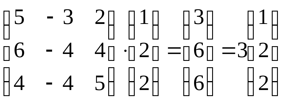
Once the (exact) value of an eigenvalue is known, the corresponding eigenvectors can be found by finding nonzero solutions of the eigenvalue equation, that becomes a system of linear equations with known coefficients. For example, once it is known that 6 is an eigenvalue of the matrix

${displaystyle A={begin{bmatrix}4&1\6&3end{bmatrix}}}$

we can find its eigenvectors by solving the equation Av=6v , that is

${displaystyle {begin{bmatrix}4&1\6&3end{bmatrix}}{begin{bmatrix}x\yend{bmatrix}}=6cdot {begin{bmatrix}x\yend{bmatrix}}}$

This matrix equation is equivalent to two linear equations

${displaystyle left{{begin{aligned}4x+y&=6x\6x+3y&=6yend{aligned}}right.}$

that is ${displaystyle left{{begin{aligned}-2x+y&=0\6x-3y&=0end{aligned}}right.}$

Both equations reduce to the single linear equation y=2x . Therefore, any vector of the form ${displaystyle {begin{bmatrix}a&2aend{bmatrix}}^{textsf {T}}}$ , for any nonzero real number , is an eigenvector of with eigenvalue .

The matrix above has another eigenvalue . A similar calculation shows that the corresponding eigenvectors are the nonzero solutions of 3x+y=0 , that is, any vector of the form ${displaystyle {begin{bmatrix}b&-3bend{bmatrix}}^{textsf {T}}}$ , for any nonzero real number .

Simple iterative methods[edit]

The converse approach, of first seeking the eigenvectors and then determining each eigenvalue from its eigenvector, turns out to be far more tractable for computers. The easiest algorithm here consists of picking an arbitrary starting vector and then repeatedly multiplying it with the matrix (optionally normalizing the vector to keep its elements of reasonable size); this makes the vector converge towards an eigenvector. A variation is to instead multiply the vector by $(A-mu I)^{{-1}}$ ; this causes it to converge to an eigenvector of the eigenvalue closest to .

If is (a good approximation of) an eigenvector of , then the corresponding eigenvalue can be computed as

${displaystyle lambda ={frac {mathbf {v} ^{*}Amathbf {v} }{mathbf {v} ^{*}mathbf {v} }}}$

where ${displaystyle mathbf {v} ^{*}}$ denotes the conjugate transpose of .

Modern methods[edit]

Efficient, accurate methods to compute eigenvalues and eigenvectors of arbitrary matrices were not known until the QR algorithm was designed in 1961.^[43] Combining the Householder transformation with the LU decomposition results in an algorithm with better convergence than the QR algorithm.^{[citation needed]} For large Hermitian sparse matrices, the Lanczos algorithm is one example of an efficient iterative method to compute eigenvalues and eigenvectors, among several other possibilities.^[43]

Most numeric methods that compute the eigenvalues of a matrix also determine a set of corresponding eigenvectors as a by-product of the computation, although sometimes implementors choose to discard the eigenvector information as soon as it is no longer needed.

Applications[edit]

Eigenvalues of geometric transformations[edit]

The following table presents some example transformations in the plane along with their 2×2 matrices, eigenvalues, and eigenvectors.

Eigenvalues of geometric transformations

	Scaling	Unequal scaling	Rotation	Horizontal shear	Hyperbolic rotation
Illustration
Matrix	${displaystyle {begin{bmatrix}k&0\0&kend{bmatrix}}}$	${displaystyle {begin{bmatrix}k_{1}&0\0&k_{2}end{bmatrix}}}$	${displaystyle {begin{bmatrix}cos theta &-sin theta \sin theta &cos theta end{bmatrix}}}$	${displaystyle {begin{bmatrix}1&k\0&1end{bmatrix}}}$	${displaystyle {begin{bmatrix}cosh varphi &sinh varphi \sinh varphi &cosh varphi end{bmatrix}}}$
Characteristic polynomial	$(lambda -k)^{2}$	$(lambda -k_{1})(lambda -k_{2})$	${displaystyle lambda ^{2}-2cos(theta )lambda +1}$	$(lambda -1)^{2}$	${displaystyle lambda ^{2}-2cosh(varphi )lambda +1}$
Eigenvalues, $lambda _{i}$	$lambda _{1}=lambda _{2}=k$	${displaystyle {begin{aligned}lambda _{1}&=k_{1}\lambda _{2}&=k_{2}end{aligned}}}$	${displaystyle {begin{aligned}lambda _{1}&=e^{itheta }\&=cos theta +isin theta \lambda _{2}&=e^{-itheta }\&=cos theta -isin theta end{aligned}}}$	$lambda _{1}=lambda _{2}=1$	${displaystyle {begin{aligned}lambda _{1}&=e^{varphi }\&=cosh varphi +sinh varphi \lambda _{2}&=e^{-varphi }\&=cosh varphi -sinh varphi end{aligned}}}$
Algebraic mult., ${displaystyle mu _{i}=mu (lambda _{i})}$	$mu _{1}=2$	${displaystyle {begin{aligned}mu _{1}&=1\mu _{2}&=1end{aligned}}}$	${displaystyle {begin{aligned}mu _{1}&=1\mu _{2}&=1end{aligned}}}$	$mu _{1}=2$	${displaystyle {begin{aligned}mu _{1}&=1\mu _{2}&=1end{aligned}}}$
Geometric mult., $gamma _{i}=gamma (lambda _{i})$	$gamma _{1}=2$	${displaystyle {begin{aligned}gamma _{1}&=1\gamma _{2}&=1end{aligned}}}$	${displaystyle {begin{aligned}gamma _{1}&=1\gamma _{2}&=1end{aligned}}}$	$gamma _{1}=1$	${displaystyle {begin{aligned}gamma _{1}&=1\gamma _{2}&=1end{aligned}}}$
Eigenvectors	All nonzero vectors	${displaystyle {begin{aligned}mathbf {u} _{1}&={begin{bmatrix}1\0end{bmatrix}}\mathbf {u} _{2}&={begin{bmatrix}0\1end{bmatrix}}end{aligned}}}$	${displaystyle {begin{aligned}mathbf {u} _{1}&={begin{bmatrix}1\-iend{bmatrix}}\mathbf {u} _{2}&={begin{bmatrix}1\+iend{bmatrix}}end{aligned}}}$	${displaystyle mathbf {u} _{1}={begin{bmatrix}1\0end{bmatrix}}}$	${displaystyle {begin{aligned}mathbf {u} _{1}&={begin{bmatrix}1\1end{bmatrix}}\mathbf {u} _{2}&={begin{bmatrix}1\-1end{bmatrix}}end{aligned}}}$

The characteristic equation for a rotation is a quadratic equation with discriminant $D=-4(sin theta )^{2}$ , which is a negative number whenever θ is not an integer multiple of 180°. Therefore, except for these special cases, the two eigenvalues are complex numbers, ; and all eigenvectors have non-real entries. Indeed, except for those special cases, a rotation changes the direction of every nonzero vector in the plane.

A linear transformation that takes a square to a rectangle of the same area (a squeeze mapping) has reciprocal eigenvalues.

Schrödinger equation[edit]

An example of an eigenvalue equation where the transformation is represented in terms of a differential operator is the time-independent Schrödinger equation in quantum mechanics:

$Hpsi _{E}=Epsi _{E},$

where , the Hamiltonian, is a second-order differential operator and $psi _{E}$ , the wavefunction, is one of its eigenfunctions corresponding to the eigenvalue , interpreted as its energy.

However, in the case where one is interested only in the bound state solutions of the Schrödinger equation, one looks for $psi _{E}$ within the space of square integrable functions. Since this space is a Hilbert space with a well-defined scalar product, one can introduce a basis set in which $psi _{E}$ and can be represented as a one-dimensional array (i.e., a vector) and a matrix respectively. This allows one to represent the Schrödinger equation in a matrix form.

The bra–ket notation is often used in this context. A vector, which represents a state of the system, in the Hilbert space of square integrable functions is represented by $|Psi _{E}rangle$ . In this notation, the Schrödinger equation is:

$H|Psi _{E}rangle =E|Psi _{E}rangle$

where $|Psi _{E}rangle$ is an eigenstate of and represents the eigenvalue. is an observable self-adjoint operator, the infinite-dimensional analog of Hermitian matrices. As in the matrix case, in the equation above $H|Psi _{E}rangle$ is understood to be the vector obtained by application of the transformation to $|Psi _{E}rangle$ .

Wave transport[edit]

Light, acoustic waves, and microwaves are randomly scattered numerous times when traversing a static disordered system. Even though multiple scattering repeatedly randomizes the waves, ultimately coherent wave transport through the system is a deterministic process which can be described by a field transmission matrix .^[44]^[45] The eigenvectors of the transmission operator ${displaystyle mathbf {t} ^{dagger }mathbf {t} }$ form a set of disorder-specific input wavefronts which enable waves to couple into the disordered system’s eigenchannels: the independent pathways waves can travel through the system. The eigenvalues, tau , of ${displaystyle mathbf {t} ^{dagger }mathbf {t} }$ correspond to the intensity transmittance associated with each eigenchannel. One of the remarkable properties of the transmission operator of diffusive systems is their bimodal eigenvalue distribution with ${displaystyle tau _{max }=1}$ and ${displaystyle tau _{min }=0}$ .^[45] Furthermore, one of the striking properties of open eigenchannels, beyond the perfect transmittance, is the statistically robust spatial profile of the eigenchannels.^[46]

Molecular orbitals[edit]

In quantum mechanics, and in particular in atomic and molecular physics, within the Hartree–Fock theory, the atomic and molecular orbitals can be defined by the eigenvectors of the Fock operator. The corresponding eigenvalues are interpreted as ionization potentials via Koopmans’ theorem. In this case, the term eigenvector is used in a somewhat more general meaning, since the Fock operator is explicitly dependent on the orbitals and their eigenvalues. Thus, if one wants to underline this aspect, one speaks of nonlinear eigenvalue problems. Such equations are usually solved by an iteration procedure, called in this case self-consistent field method. In quantum chemistry, one often represents the Hartree–Fock equation in a non-orthogonal basis set. This particular representation is a generalized eigenvalue problem called Roothaan equations.

Geology and glaciology[edit]

In geology, especially in the study of glacial till, eigenvectors and eigenvalues are used as a method by which a mass of information of a clast fabric’s constituents’ orientation and dip can be summarized in a 3-D space by six numbers. In the field, a geologist may collect such data for hundreds or thousands of clasts in a soil sample, which can only be compared graphically such as in a Tri-Plot (Sneed and Folk) diagram,^[47]^[48] or as a Stereonet on a Wulff Net.^[49]

The output for the orientation tensor is in the three orthogonal (perpendicular) axes of space. The three eigenvectors are ordered ${displaystyle mathbf {v} _{1},mathbf {v} _{2},mathbf {v} _{3}}$ by their eigenvalues $E_{1}geq E_{2}geq E_{3}$ ;^[50]
${displaystyle mathbf {v} _{1}}$ then is the primary orientation/dip of clast, ${displaystyle mathbf {v} _{2}}$ is the secondary and ${displaystyle mathbf {v} _{3}}$ is the tertiary, in terms of strength. The clast orientation is defined as the direction of the eigenvector, on a compass rose of 360°. Dip is measured as the eigenvalue, the modulus of the tensor: this is valued from 0° (no dip) to 90° (vertical). The relative values of $E_{1}$ , $E_{2}$ , and $E_{3}$ are dictated by the nature of the sediment’s fabric. If $E_{1}=E_{2}=E_{3}$ , the fabric is said to be isotropic. If $E_{1}=E_{2}>E_{3}$ , the fabric is said to be planar. If $E_{1}>E_{2}>E_{3}$ , the fabric is said to be linear.^[51]

Principal component analysis[edit]

PCA of the multivariate Gaussian distribution centered at with a standard deviation of 3 in roughly the direction and of 1 in the orthogonal direction. The vectors shown are unit eigenvectors of the (symmetric, positive-semidefinite) covariance matrix scaled by the square root of the corresponding eigenvalue. Just as in the one-dimensional case, the square root is taken because the standard deviation is more readily visualized than the variance.

The eigendecomposition of a symmetric positive semidefinite (PSD) matrix yields an orthogonal basis of eigenvectors, each of which has a nonnegative eigenvalue. The orthogonal decomposition of a PSD matrix is used in multivariate analysis, where the sample covariance matrices are PSD. This orthogonal decomposition is called principal component analysis (PCA) in statistics. PCA studies linear relations among variables. PCA is performed on the covariance matrix or the correlation matrix (in which each variable is scaled to have its sample variance equal to one). For the covariance or correlation matrix, the eigenvectors correspond to principal components and the eigenvalues to the variance explained by the principal components. Principal component analysis of the correlation matrix provides an orthogonal basis for the space of the observed data: In this basis, the largest eigenvalues correspond to the principal components that are associated with most of the covariability among a number of observed data.

Principal component analysis is used as a means of dimensionality reduction in the study of large data sets, such as those encountered in bioinformatics. In Q methodology, the eigenvalues of the correlation matrix determine the Q-methodologist’s judgment of practical significance (which differs from the statistical significance of hypothesis testing; cf. criteria for determining the number of factors). More generally, principal component analysis can be used as a method of factor analysis in structural equation modeling.

Vibration analysis[edit]

Mode shape of a tuning fork at eigenfrequency 440.09 Hz

Eigenvalue problems occur naturally in the vibration analysis of mechanical structures with many degrees of freedom. The eigenvalues are the natural frequencies (or eigenfrequencies) of vibration, and the eigenvectors are the shapes of these vibrational modes. In particular, undamped vibration is governed by

that is, acceleration is proportional to position (i.e., we expect to be sinusoidal in time).

In dimensions, becomes a mass matrix and a stiffness matrix. Admissible solutions are then a linear combination of solutions to the generalized eigenvalue problem

${displaystyle kx=omega ^{2}mx}$

where $omega ^{2}$ is the eigenvalue and omega is the (imaginary) angular frequency. The principal vibration modes are different from the principal compliance modes, which are the eigenvectors of alone. Furthermore, damped vibration, governed by

leads to a so-called quadratic eigenvalue problem,

${displaystyle left(omega ^{2}m+omega c+kright)x=0.}$

This can be reduced to a generalized eigenvalue problem by algebraic manipulation at the cost of solving a larger system.

The orthogonality properties of the eigenvectors allows decoupling of the differential equations so that the system can be represented as linear summation of the eigenvectors. The eigenvalue problem of complex structures is often solved using finite element analysis, but neatly generalize the solution to scalar-valued vibration problems.

Eigenfaces[edit]

In image processing, processed images of faces can be seen as vectors whose components are the brightnesses of each pixel.^[52] The dimension of this vector space is the number of pixels. The eigenvectors of the covariance matrix associated with a large set of normalized pictures of faces are called eigenfaces; this is an example of principal component analysis. They are very useful for expressing any face image as a linear combination of some of them. In the facial recognition branch of biometrics, eigenfaces provide a means of applying data compression to faces for identification purposes. Research related to eigen vision systems determining hand gestures has also been made.

Similar to this concept, eigenvoices represent the general direction of variability in human pronunciations of a particular utterance, such as a word in a language. Based on a linear combination of such eigenvoices, a new voice pronunciation of the word can be constructed. These concepts have been found useful in automatic speech recognition systems for speaker adaptation.

Tensor of moment of inertia[edit]

In mechanics, the eigenvectors of the moment of inertia tensor define the principal axes of a rigid body. The tensor of moment of inertia is a key quantity required to determine the rotation of a rigid body around its center of mass.

Stress tensor[edit]

In solid mechanics, the stress tensor is symmetric and so can be decomposed into a diagonal tensor with the eigenvalues on the diagonal and eigenvectors as a basis. Because it is diagonal, in this orientation, the stress tensor has no shear components; the components it does have are the principal components.

Graphs[edit]

In spectral graph theory, an eigenvalue of a graph is defined as an eigenvalue of the graph’s adjacency matrix , or (increasingly) of the graph’s Laplacian matrix due to its discrete Laplace operator, which is either (sometimes called the combinatorial Laplacian) or ${displaystyle I-D^{-1/2}AD^{-1/2}}$ (sometimes called the normalized Laplacian), where is a diagonal matrix with ${displaystyle D_{ii}}$ equal to the degree of vertex $v_{i}$ , and in $D^{-1/2}$ , the th diagonal entry is ${textstyle 1/{sqrt {deg(v_{i})}}}$ . The th principal eigenvector of a graph is defined as either the eigenvector corresponding to the th largest or th smallest eigenvalue of the Laplacian. The first principal eigenvector of the graph is also referred to merely as the principal eigenvector.

The principal eigenvector is used to measure the centrality of its vertices. An example is Google’s PageRank algorithm. The principal eigenvector of a modified adjacency matrix of the World Wide Web graph gives the page ranks as its components. This vector corresponds to the stationary distribution of the Markov chain represented by the row-normalized adjacency matrix; however, the adjacency matrix must first be modified to ensure a stationary distribution exists. The second smallest eigenvector can be used to partition the graph into clusters, via spectral clustering. Other methods are also available for clustering.

Basic reproduction number[edit]

The basic reproduction number ( $R_{0}$ ) is a fundamental number in the study of how infectious diseases spread. If one infectious person is put into a population of completely susceptible people, then $R_{0}$ is the average number of people that one typical infectious person will infect. The generation time of an infection is the time, $t_{G}$ , from one person becoming infected to the next person becoming infected. In a heterogeneous population, the next generation matrix defines how many people in the population will become infected after time $t_{G}$ has passed. $R_{0}$ is then the largest eigenvalue of the next generation matrix.^[53]^[54]

Notes[edit]

^
Note:
- In 1751, Leonhard Euler proved that any body has a principal axis of rotation: Leonhard Euler (presented: October 1751; published: 1760) «Du mouvement d’un corps solide quelconque lorsqu’il tourne autour d’un axe mobile» (On the movement of any solid body while it rotates around a moving axis), Histoire de l’Académie royale des sciences et des belles lettres de Berlin, pp. 176–227. On p. 212, Euler proves that any body contains a principal axis of rotation: «Théorem. 44. De quelque figure que soit le corps, on y peut toujours assigner un tel axe, qui passe par son centre de gravité, autour duquel le corps peut tourner librement & d’un mouvement uniforme.» (Theorem. 44. Whatever be the shape of the body, one can always assign to it such an axis, which passes through its center of gravity, around which it can rotate freely and with a uniform motion.)
- In 1755, Johann Andreas Segner proved that any body has three principal axes of rotation: Johann Andreas Segner, Specimen theoriae turbinum [Essay on the theory of tops (i.e., rotating bodies)] ( Halle («Halae»), (Germany): Gebauer, 1755). (https://books.google.com/books?id=29 p. xxviiii [29]), Segner derives a third-degree equation in t, which proves that a body has three principal axes of rotation. He then states (on the same page): «Non autem repugnat tres esse eiusmodi positiones plani HM, quia in aequatione cubica radices tres esse possunt, et tres tangentis t valores.» (However, it is not inconsistent [that there] be three such positions of the plane HM, because in cubic equations, [there] can be three roots, and three values of the tangent t.)
- The relevant passage of Segner’s work was discussed briefly by Arthur Cayley. See: A. Cayley (1862) «Report on the progress of the solution of certain special problems of dynamics,» Report of the Thirty-second meeting of the British Association for the Advancement of Science; held at Cambridge in October 1862, 32: 184–252; see especially pp. 225–226.
^ Kline 1972, pp. 807–808 Augustin Cauchy (1839) «Mémoire sur l’intégration des équations linéaires» (Memoir on the integration of linear equations), Comptes rendus, 8: 827–830, 845–865, 889–907, 931–937. From p. 827: «On sait d’ailleurs qu’en suivant la méthode de Lagrange, on obtient pour valeur générale de la variable prinicipale une fonction dans laquelle entrent avec la variable principale les racines d’une certaine équation que j’appellerai l’équation caractéristique, le degré de cette équation étant précisément l’order de l’équation différentielle qu’il s’agit d’intégrer.» (One knows, moreover, that by following Lagrange’s method, one obtains for the general value of the principal variable a function in which there appear, together with the principal variable, the roots of a certain equation that I will call the «characteristic equation», the degree of this equation being precisely the order of the differential equation that must be integrated.)
^
See:
- David Hilbert (1904) «Grundzüge einer allgemeinen Theorie der linearen Integralgleichungen. (Erste Mitteilung)» (Fundamentals of a general theory of linear integral equations. (First report)), Nachrichten von der Gesellschaft der Wissenschaften zu Göttingen, Mathematisch-Physikalische Klasse (News of the Philosophical Society at Göttingen, mathematical-physical section), pp. 49–91. From p. 51: «Insbesondere in dieser ersten Mitteilung gelange ich zu Formeln, die die Entwickelung einer willkürlichen Funktion nach gewissen ausgezeichneten Funktionen, die ich ‘Eigenfunktionen’ nenne, liefern: …» (In particular, in this first report I arrive at formulas that provide the [series] development of an arbitrary function in terms of some distinctive functions, which I call eigenfunctions: … ) Later on the same page: «Dieser Erfolg ist wesentlich durch den Umstand bedingt, daß ich nicht, wie es bisher geschah, in erster Linie auf den Beweis für die Existenz der Eigenwerte ausgehe, … « (This success is mainly attributable to the fact that I do not, as it has happened until now, first of all aim at a proof of the existence of eigenvalues, … )
- For the origin and evolution of the terms eigenvalue, characteristic value, etc., see: Earliest Known Uses of Some of the Words of Mathematics (E)
^ For a proof of this lemma, see Roman 2008, Theorem 8.2 on p. 186; Shilov 1977, p. 109; Hefferon 2001, p. 364; Beezer 2006, Theorem EDELI on p. 469; and Lemma for linear independence of eigenvectors
^ By doing Gaussian elimination over formal power series truncated to terms it is possible to get away with $O(n^{4})$ operations, but that does not take combinatorial explosion into account.

Citations[edit]

^ Burden & Faires 1993, p. 401.
^ Roman 2008, p. 185 §8
^ ^a ^b Herstein 1964, pp. 228, 229.
^ ^a ^b Nering 1970, p. 38.
^ Weisstein n.d.
^ Betteridge 1965.
^ ^a ^b «Eigenvector and Eigenvalue». www.mathsisfun.com. Retrieved 19 August 2020.
^ Press et al. 2007, p. 536.
^ Wolfram.com: Eigenvector.
^ ^a ^b ^c ^d Nering 1970, p. 107.
^ Hawkins 1975, §2.
^ ^a ^b ^c ^d Hawkins 1975, §3.
^ Kline 1972, p. 673.
^ ^a ^b Kline 1972, pp. 807–808.
^ Kline 1972, pp. 715–716.
^ Kline 1972, pp. 706–707.
^ Kline 1972, p. 1063, p..
^ Aldrich 2006.
^ Francis 1961, pp. 265–271.
^ Kublanovskaya 1962.
^ Golub & Van Loan 1996, §7.3.
^ Meyer 2000, §7.3.
^ Cornell University Department of Mathematics (2016) Lower-Level Courses for Freshmen and Sophomores. Accessed on 2016-03-27.
^ University of Michigan Mathematics (2016) Math Course Catalogue Archived 2015-11-01 at the Wayback Machine. Accessed on 2016-03-27.
^ Press et al. 2007, p. 38.
^ Fraleigh 1976, p. 358.
^ ^a ^b ^c Golub & Van Loan 1996, p. 316.
^ Anton 1987, pp. 305, 307.
^ ^a ^b Beauregard & Fraleigh 1973, p. 307.
^ Herstein 1964, p. 272.
^ Nering 1970, pp. 115–116.
^ Herstein 1964, p. 290.
^ Nering 1970, p. 116.
^ Wolchover 2019.
^ ^a ^b Denton et al. 2022.
^ Van Mieghem 2014.
^ Korn & Korn 2000, Section 14.3.5a.
^ Friedberg, Insel & Spence 1989, p. 217.
^ Roman 2008, p. 186 §8
^ Nering 1970, p. 107; Shilov 1977, p. 109 Lemma for the eigenspace
^ Lipschutz & Lipson 2002, p. 111.
^ Roman 2008, p. 189 §8.
^ ^a ^b ^c ^d Trefethen & Bau 1997.
^ Vellekoop & Mosk 2007, pp. 2309–2311.
^ ^a ^b Rotter & Gigan 2017, p. 15005.
^ Bender et al. 2020, p. 165901.
^ Graham & Midgley 2000, pp. 1473–1477.
^ Sneed & Folk 1958, pp. 114–150.
^ Knox-Robinson & Gardoll 1998, p. 243.
^ Busche, Christian; Schiller, Beate. «Endogene Geologie — Ruhr-Universität Bochum». www.ruhr-uni-bochum.de.
^ Benn & Evans 2004, pp. 103–107.
^ Xirouhakis, Votsis & Delopoulus 2004.
^ Diekmann, Heesterbeek & Metz 1990, pp. 365–382.
^ Heesterbeek & Diekmann 2000.

Sources[edit]

Aldrich, John (2006), «Eigenvalue, eigenfunction, eigenvector, and related terms», in Miller, Jeff (ed.), Earliest Known Uses of Some of the Words of Mathematics
Anton, Howard (1987), Elementary Linear Algebra (5th ed.), New York: Wiley, ISBN 0-471-84819-0
Beauregard, Raymond A.; Fraleigh, John B. (1973), A First Course In Linear Algebra: with Optional Introduction to Groups, Rings, and Fields, Boston: Houghton Mifflin Co., ISBN 0-395-14017-X
Beezer, Robert A. (2006), A first course in linear algebra, Free online book under GNU licence, University of Puget Sound
Bender, Nicholas; Yamilov, Alexey; Yilmaz, Hasan; Cao, Hui (14 October 2020). «Fluctuations and Correlations of Transmission Eigenchannels in Diffusive Media». Physical Review Letters. 125 (16): 165901. arXiv:2004.12167. Bibcode:2020PhRvL.125p5901B. doi:10.1103/physrevlett.125.165901. ISSN 0031-9007. PMID 33124845. S2CID 216553547.
Benn, D.; Evans, D. (2004), A Practical Guide to the study of Glacial Sediments, London: Arnold, pp. 103–107
Betteridge, Harold T. (1965), The New Cassell’s German Dictionary, New York: Funk & Wagnall, LCCN 58-7924
Burden, Richard L.; Faires, J. Douglas (1993), Numerical Analysis (5th ed.), Boston: Prindle, Weber and Schmidt, ISBN 0-534-93219-3
Denton, Peter B.; Parke, Stephen J.; Tao, Terence; Zhang, Xining (January 2022). «Eigenvectors from Eigenvalues: A Survey of a Basic Identity in Linear Algebra» (PDF). Bulletin of the American Mathematical Society. 59 (1): 31–58. arXiv:1908.03795. doi:10.1090/bull/1722. S2CID 213918682. Archived (PDF) from the original on 19 January 2022.
Diekmann, O; Heesterbeek, JA; Metz, JA (1990), «On the definition and the computation of the basic reproduction ratio R0 in models for infectious diseases in heterogeneous populations», Journal of Mathematical Biology, 28 (4): 365–382, doi:10.1007/BF00178324, hdl:1874/8051, PMID 2117040, S2CID 22275430
Fraleigh, John B. (1976), A First Course In Abstract Algebra (2nd ed.), Reading: Addison-Wesley, ISBN 0-201-01984-1
Francis, J. G. F. (1961), «The QR Transformation, I (part 1)», The Computer Journal, 4 (3): 265–271, doi:10.1093/comjnl/4.3.265
Francis, J. G. F. (1962), «The QR Transformation, II (part 2)», The Computer Journal, 4 (4): 332–345, doi:10.1093/comjnl/4.4.332
Friedberg, Stephen H.; Insel, Arnold J.; Spence, Lawrence E. (1989), Linear algebra (2nd ed.), Englewood Cliffs, NJ: Prentice Hall, ISBN 0-13-537102-3
Golub, Gene H.; Van Loan, Charles F. (1996), Matrix computations (3rd ed.), Baltimore, MD: Johns Hopkins University Press, ISBN 978-0-8018-5414-9
Graham, D.; Midgley, N. (2000), «Graphical representation of particle shape using triangular diagrams: an Excel spreadsheet method», Earth Surface Processes and Landforms, 25 (13): 1473–1477, Bibcode:2000ESPL…25.1473G, doi:10.1002/1096-9837(200012)25:13<1473::AID-ESP158>3.0.CO;2-C, S2CID 128825838
Hawkins, T. (1975), «Cauchy and the spectral theory of matrices», Historia Mathematica, 2: 1–29, doi:10.1016/0315-0860(75)90032-4
Heesterbeek, J. A. P.; Diekmann, Odo (2000), Mathematical epidemiology of infectious diseases, Wiley series in mathematical and computational biology, West Sussex, England: John Wiley & Sons
Hefferon, Jim (2001), Linear Algebra, Colchester, VT: Online book, St Michael’s College
Herstein, I. N. (1964), Topics In Algebra, Waltham: Blaisdell Publishing Company, ISBN 978-1114541016
Kline, Morris (1972), Mathematical thought from ancient to modern times, Oxford University Press, ISBN 0-19-501496-0
Knox-Robinson, C.; Gardoll, Stephen J. (1998), «GIS-stereoplot: an interactive stereonet plotting module for ArcView 3.0 geographic information system», Computers & Geosciences, 24 (3): 243, Bibcode:1998CG…..24..243K, doi:10.1016/S0098-3004(97)00122-2
Korn, Granino A.; Korn, Theresa M. (2000), «Mathematical Handbook for Scientists and Engineers: Definitions, Theorems, and Formulas for Reference and Review», New York: McGraw-Hill (2nd Revised ed.), Bibcode:1968mhse.book…..K, ISBN 0-486-41147-8
Kublanovskaya, Vera N. (1962), «On some algorithms for the solution of the complete eigenvalue problem», USSR Computational Mathematics and Mathematical Physics, 1 (3): 637–657, doi:10.1016/0041-5553(63)90168-X
Lipschutz, Seymour; Lipson, Marc (12 August 2002). Schaum’s Easy Outline of Linear Algebra. McGraw Hill Professional. p. 111. ISBN 978-007139880-0.
Meyer, Carl D. (2000), Matrix analysis and applied linear algebra, Philadelphia: Society for Industrial and Applied Mathematics (SIAM), ISBN 978-0-89871-454-8
Nering, Evar D. (1970), Linear Algebra and Matrix Theory (2nd ed.), New York: Wiley, LCCN 76091646
Press, William H.; Teukolsky, Saul A.; Vetterling, William T.; Flannery, Brian P. (2007), Numerical Recipes: The Art of Scientific Computing (3rd ed.), ISBN 978-0521880688
Roman, Steven (2008), Advanced linear algebra (3rd ed.), New York: Springer Science + Business Media, ISBN 978-0-387-72828-5
Rotter, Stefan; Gigan, Sylvain (2 March 2017). «Light fields in complex media: Mesoscopic scattering meets wave control». Reviews of Modern Physics. 89 (1): 015005. arXiv:1702.05395. Bibcode:2017RvMP…89a5005R. doi:10.1103/RevModPhys.89.015005. S2CID 119330480.
Shilov, Georgi E. (1977), Linear algebra, Translated and edited by Richard A. Silverman, New York: Dover Publications, ISBN 0-486-63518-X
Sneed, E. D.; Folk, R. L. (1958), «Pebbles in the lower Colorado River, Texas, a study of particle morphogenesis», Journal of Geology, 66 (2): 114–150, Bibcode:1958JG…..66..114S, doi:10.1086/626490, S2CID 129658242
Trefethen, Lloyd N.; Bau, David (1997), Numerical Linear Algebra, SIAM
Van Mieghem, Piet (18 January 2014). «Graph eigenvectors, fundamental weights and centrality metrics for nodes in networks». arXiv:1401.4580 [math.SP].
Vellekoop, I. M.; Mosk, A. P. (15 August 2007). «Focusing coherent light through opaque strongly scattering media». Optics Letters. 32 (16): 2309–2311. Bibcode:2007OptL…32.2309V. doi:10.1364/OL.32.002309. ISSN 1539-4794. PMID 17700768. S2CID 45359403.
Weisstein, Eric W. «Eigenvector». mathworld.wolfram.com. Retrieved 4 August 2019.
Weisstein, Eric W. (n.d.). «Eigenvalue». mathworld.wolfram.com. Retrieved 19 August 2020.
Wolchover, Natalie (13 November 2019). «Neutrinos Lead to Unexpected Discovery in Basic Math». Quanta Magazine. Retrieved 27 November 2019.
Xirouhakis, A.; Votsis, G.; Delopoulus, A. (2004), Estimation of 3D motion and structure of human faces (PDF), National Technical University of Athens

External links[edit]

What are Eigen Values? – non-technical introduction from PhysLink.com’s «Ask the Experts»
Eigen Values and Eigen Vectors Numerical Examples – Tutorial and Interactive Program from Revoledu.
Introduction to Eigen Vectors and Eigen Values – lecture from Khan Academy
Eigenvectors and eigenvalues | Essence of linear algebra, chapter 10 – A visual explanation with 3Blue1Brown
Matrix Eigenvectors Calculator from Symbolab (Click on the bottom right button of the 2×12 grid to select a matrix size. Select an size (for a square matrix), then fill out the entries numerically and click on the Go button. It can accept complex numbers as well.)

Theory[edit]

Computation of Eigenvalues
Numerical solution of eigenvalue problems Edited by Zhaojun Bai, James Demmel, Jack Dongarra, Axel Ruhe, and Henk van der Vorst

Источник

Характеристическое уравнение линейного оператора А: L → L, действующего в n-мерном линейном пространстве L, — это алгебраическое уравнение n-й степени с действительными коэффициентами. Среди его корней могут быть комплексные числа, но эти корни не относят к собственным значениям линейного оператора, так как, согласно определению, собственное значение линейного оператора — действительное число. Чтобы комплексные корни характеристического уравнения можно было рассматривать как собственные значения линейного оператора, в линейном пространстве должно быть определено умножение вектора на любые комплексные числа.

Как следует из доказательства теоремы 5.3, чтобы вычислить собственные значения линейного оператора А и найти его собственные векторы, нужно выполнить следующие операции:

— выбрать в линейном пространстве базис и сопоставить А матрицу А этого линейного оператора в выбранном базисе;

— составить характеристическое уравнение det (А — λЕ) = 0 и найти все его действительные корни λ_k, которые и будут собственными значениями линейного оператора;

— для каждого собственного значения λ_k найти фундаментальную систему решений
для однородной системы линейных алгебраических уравнений (СЛАУ) (А — λ_kЕ)х = 0. Столбцы фундаментальной системы решений представляют собой координаты векторов некоторого базиса в собственном подпространстве £(А, λ_k) линейного оператора А.

Любой собственный вектор с собственным значением λ_k принадлежит подпространству £(А,λ_k), и, следовательно, найденный базис в этом подпространстве позволяет представить любой собственный вектор с собственным значением λ_k.

Пример 5.4. Найдем собственные векторы и собственные значения линейного оператора А, имеющего в некотором базисе матрицу

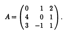
В соответствии с описанной процедурой необходимо выполнить три действия. Первое действие можно опустить, так как оператор уже представлен своей матрицей в некотором базисе. Выполняем дальнейшие действия.

2) Находим собственные значения, решая характеристическое уравнение матрицы:

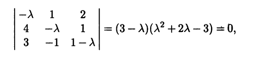
откуда λ₁ = -3, λ₂ = 1, λ₃ = 3.

3) Находим столбцы координат собственных векторов, ре-шая для каждого из трех собственных значений однородную СЛАУ

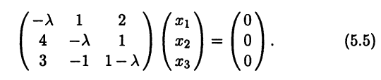
3а) Для λ = λ₁ = -3 система (5.5) имеет вид

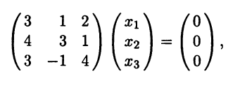
или

Ранг матрицы этой системы равен 2:

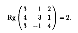
Поэтому размерность линейного пространства решений систе-мы равна 3 — 2 = 1. Фундаментальная система решений содер-жит одно решение, например

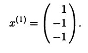
Все множество собственных векторов линейного оператора с собственным значением λ₁ = -3 в координатной форме имеет вид

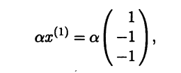
где α — произвольное ненулевое действительное число.

3б) При λ = λ₂ = 1 система (5.5) имеет вид

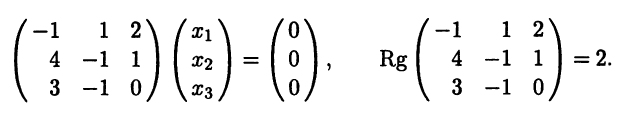
Как и в предыдущем случае, размерность линейного простран-ства решений равна 2 — 1 = 1 и фундаментальная система решений содержит одно решение. Выберем следующее:

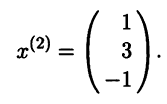
Все множество собственных векторов с собственным значением λ = -1 в координатной форме имеет вид

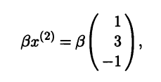
где β — произвольное ненулевое действительное число.

3в) Для λ = λ₃ = 3 аналогично предыдущим двум случаям находим столбец координат одного из собственных векторов, например

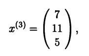
который порождает собственное подпространство линейного оператора А, отвечающее собственному значению λ = 3.

Пример 5.5. Найдем собственные значения линейного оператора А, действующего в n-мерном линейном пространстве, матрица А которого в некотором базисе является верхней треугольной порядка n:

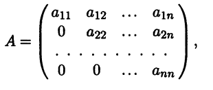
причем все ее диагональные элементы а_ii попарно различны, т.е. а_ii ≠ a_jj при i ≠ j.

Составляем характеристическое уравнение матрицы А:

det(А — λЕ) = (а₁₁ — λ)(а₂₂ — λ) … (а_nn — λ) = 0

(определитель верхней треугольной матрицы равен произведе-нию ее диагональных элементов). Находим все действительные корни этого уравнения:

λ_k = a_kk, k = 1,n

Как видим, линейный оператор А имеет n попарно различных собственных значений.

Отметим, что пересечение любых двух собственных подпространств линейного оператора содержит лишь нулевой вектор, так как собственный вектор не может отвечать двум различным собственным значениям. Поэтому собственные подпространства линейного оператора образуют прямую сумму, а размерность прямой суммы линейных подпространств, согласно следствию из теоремы 2.5, равна сумме их размерностей. Из этих соображений следует, что каждое из n собственных подпространств рассматриваемого линейного оператора является одномерным, так как их размерность не может быть меньше, но если бы одно из подпространств имело размерность больше единицы, то суммарная их размерность превышала бы размерность самого линейного пространства.

Итак, все собственные подпространства линейного операто-ра в нашем случае одномерны. Рассмотрим то из них, которое отвечает собственному значению λ_r = а_rr, где 1 ≤ r ≤ n. Соответствующий собственный вектор имеет столбец координат, который является ненулевым решением однородной СЛАУ

(А — a_rrЕ)х = 0. (5.6)

Достаточно очевидно, что ранг матрицы системы (5.6) равен n — 1, а базисный минор для этой матрицы получается вычер-киванием r-й строки и r-го столбца.

Наиболее просто решение системы (5.6) выглядит для r = 1. В этом случае собственным является вектор x₁ со столбцом координат (1 0 … 0)^T . При r = 2 все координаты собственного вектора, начиная с третьей, будут равны нулю, так как они удовлетворяют системе

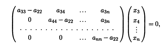
получающейся выбрасыванием первых двух уравнений. Второе уравнение вытекает из всех последующих и может быть опуще-но, а первое уравнение определяет связь между первыми двумя координатами. Мы получаем, что собственному значению а₂₂ отвечает вектор x₂ со столбцом координат (-a₁₂ a₁₁ 0 … 0)^T . Собственному значению a₃₃ отвечает вектор x₃ со столбцом координат (x₁₃ x₂₃ x₃₃ 0 … 0)^T , у которого лишь первые три координаты отличны от нуля. Эти три координаты удовлетворяют однородной системе из двух уравнений

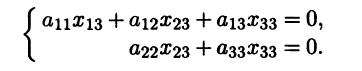
Эти рассуждения можно продолжить.

Пример 5.6. Преобразование поворота в V₃ на заданный острый угол вокруг некоторой оси — это линейный оператор. Его собственными векторами являются векторы, коллинеарные оси поворота. Например, если поворот выполняется вокруг оси Оz, то матрица оператора в базисе i, j, k будет иметь вид

а его собственными векторами будут векторы со столбцами координат вида λ(0 0 1)^T , λ ≠ 0.

Линейные операции над векторами
Базис. Cкалярное произведение
Векторное и смешанное произведения векторов
Декартова система координат. прямая на плоскости
Плоскость в пространстве
Прямая в пространстве
Кривые второго порядка — I
Кривые второго порядка — II
Поверхности второго порядка
Матрицы и операции с ними
Обратная матрица
Ранг матрицы
Системы линейных алгебраических уравнений
Свойства решений однородных и неоднородных СЛАУ

Источник

Собственные векторы и собственные значения матрицы

Свойства собственных векторов

Нахождение собственных векторов и собственных значений матрицы

1. Основные понятия.

2. Свойства собственных векторов.

3 Нахождение собственных значений и собственных векторов.

Formal definition[edit]

Overview[edit]

History[edit]

Eigenvalues and eigenvectors of matrices[edit]

Eigenvalues and the characteristic polynomial[edit]

Algebraic multiplicity[edit]

Eigenspaces, geometric multiplicity, and the eigenbasis for matrices[edit]

Additional properties of eigenvalues[edit]

Left and right eigenvectors[edit]

Diagonalization and the eigendecomposition[edit]

Variational characterization[edit]

Matrix examples[edit]

Two-dimensional matrix example[edit]

Three-dimensional matrix example[edit]

Three-dimensional matrix example with complex eigenvalues[edit]

Diagonal matrix example[edit]

Triangular matrix example[edit]

Matrix with repeated eigenvalues example[edit]

Eigenvector-eigenvalue identity[edit]

Eigenvalues and eigenfunctions of differential operators[edit]

Derivative operator example[edit]

General definition[edit]

Eigenspaces, geometric multiplicity, and the eigenbasis[edit]

Spectral theory[edit]

Associative algebras and representation theory[edit]

Dynamic equations[edit]

Calculation[edit]

Classical method[edit]

Eigenvalues[edit]

Eigenvectors[edit]

Simple iterative methods[edit]

Modern methods[edit]

Applications[edit]

Eigenvalues of geometric transformations[edit]

Schrödinger equation[edit]

Wave transport[edit]

Molecular orbitals[edit]

Geology and glaciology[edit]

Principal component analysis[edit]

Vibration analysis[edit]

Eigenfaces[edit]

Tensor of moment of inertia[edit]

Stress tensor[edit]

Graphs[edit]

Basic reproduction number[edit]

See also[edit]

Notes[edit]

Citations[edit]

Sources[edit]

Further reading[edit]

External links[edit]

Theory[edit]

Линейные операции над векторами

Базис. Cкалярное произведение

Векторное и смешанное произведения векторов

Декартова система координат. прямая на плоскости

Плоскость в пространстве

Прямая в пространстве

Кривые второго порядка — I

Кривые второго порядка — II

Поверхности второго порядка

Матрицы и операции с ними

Обратная матрица

Ранг матрицы

Системы линейных алгебраических уравнений

Свойства решений однородных и неоднородных СЛАУ