Лекция №3
План лекции:
1.Поверхностное натяжение — физический смысл.
АДСОРБЦИЯ
Поверхностная энергия стремится самопроизвольно уменьшиться. Это выражается в уменьшении межфазной поверхности или поверхностного натяжения ( s )
Вследствие этого стремления происходит адсорбция.
Адсорбция — процесс самопроизвольного перераспределения компонентов системы между поверхностным слоем и объемной фазой. Т.е. адсорбция может происходить в многокомпонентных системах, в слой переходит тот компонент, который сильнее уменьшает s .
Адсорбент — фаза определяющая форму поверхности, более плотная, может быть твердой или жидкой.
Адсорбат — вещество которое перераспределяется (газ или жидкость).
Десорбция — переход вещества из поверхностного слоя в объемную фазу.
Количественно адсорбцию описывают величиной Гиббсовской адсорбции (избыток вещества в поверхностном слое по сравнению с его количеством в объемной фазе, отнесенный к единице площади поверхности или единице массы адсорбента)
(3.1)
Г i -Гиббсовская адсорбция,
V -объем системы,
с0 -исходная концентрация адсорбата ,
с i — концентрация адсорбата в объеме,
S — площадь поверхности раздела.
Все величины в (3.1) могут быть установлены экспериментально.
Адсорбцию можно рассматривать как процесс превращения поверхностной энергии в химическую.
Выведем соотношение между поверхностным натяжением и химическими параметрами компонентов.
Если объем поверхностного слоя равен 0, то
т.к. внутр. энергия пропорциональна экстенсивным величинам, то:
полный дифференциал от тех же переменных запишется следующим образом:
dU=T dS + S dT + s dS +S d s + å m i dn i + å n i d m (3.3)
Подставляя dU из 3.2 в 3.3, получим:
3.4 и 3.5 — уравнения Гиббса для межфазной поверхности (поверхностного слоя).
Все экстенсивные величины поверхности зависят от площади поверхности , поэтому удобнее относить эти параметры к единице площади поверхности. Разделив уравнение 3.5 на площадь поверхности, получим:
=> (3.6)
Г i — поверхностный избыток компонента i в поверхностном слое (по сравнению с его равновесной концентрацией в объемной фазе), то есть величина Гиббсовской адсорбции.
Уравнение 3.6 — фундаментальное адсорбционное уравнение Гиббса. Это строгое термодинамическое соотношение, написанное для многокомпонентной системы. Однако, практиче ское его использование неудобно. Оно, например, не раскрывает зависимость поверхностного натяжения от адсорбции конкретного вещества при постоянных химических потенциалах других веществ.. Единицы величины гиббсовской адсорбции определяются единицами химического потенциала. Если потенциал отнесен к молю вещества, то величина адсорбции выражается в молях на единицу площади.
Адсорбция конкретного вещества при постоянных химических параметрах других веществ:
Принимая во внимание , что m i = m i o + RT ln ai, m i и m i o — равновесное и стандартное значения химического потенциала адсорбата i , а i — термодинамическая активность адсорбата, d m i = RT d ln ai ,получим :
для Гиббсовской адсорбции:
(3.7)
3.7. применяют только тогда, когда можно использовать концентрации вместо активностей и пренебречь изменениями концентраций других веществ при изменении концентрации одного вещества. Этим условиям удовлетворяет разбавленный раствор относительно данного компонента. В таком растворе при изменении концентрации растворенного вещества практически не изменяется концентрация растворителя. Поэтому для растворенного вещества уравнение 3.7 переходит в широко используемые адсорбционные уравнения Гиббса для неэлектролитов и электролитов
(3.8)
(3.9)
УРАВНЕНИЕ ГЕНРИ, ФРЕЙНДЛИХА, ЛЕНГМЮРА
Для описания процесса адсорбции, помимо фундаментального уравнения адсорбции Гиббса, применяют ряд других аналитических уравнений, которые называются по имени их авторов.
При незначительном заполнении адсорбента адсорбатом отношение концентрации вещества в адсорбционном слое и в объеме стремится к постоянному значению, равному кГ:
Это уравнение характеризует изотерму адсорбции при малых концентрациях адсорбата (рис.3.1, участок 1) и является аналитическим выражением закона Генри. Коэффициент кГ не зависит от концентрации и представляет собой константу распределения, характеризующую распределение вещества в адсорбционном слое по отношению к его содержанию в объемной фазе. Уравнение Генри соблюдается приближенно, но это приближение достаточно для практики.
В более общем виде зависимость адсорбции от концентрации адсорбата можно определить с помощью уравнения Фрейндлиха.
Константы адсорбции в уравнениях ленгмюра и генри
Небольшая предыстория . В ходе изучения ПАВ американский химик и физик Ирвинг Ленгмюр выдвинул и математически обосновал идею об особом строении адсорбционных слоев. Он рассматривал ненасыщенный слой как двухмерный газ. По мере того как концентрация ПАВ увеличивается, происходит процесс, аналогичный конденсации двухмерного газа – молекулы образуют двухмерную пленку, которую Ленгмюр рассматривал как двухмерную жидкость. Если концентрация ПАВ в растворе неограниченно возрастает, то наступает момент предельного насыщения адсорбционного слоя, который приобретает вид частокола, так как предполагается, что слой имеет толщину, соответствующую длине адсорбированной молекулы. При этом адсорбция достигает предела. Эта теория была названа теорией мономолекулярного слоя, или монослоя.
Теория Ирвинга Ленгмюра(1914-1918) явилась фундаментальным вкладом в учение об адсорбции. Она позволяет учесть наиболее сильные отклонения от закона Генри, связанные с ограниченностью поверхности адсорбента. Ограниченность этого параметра приводит к адсорбционному насыщению поверхности адсорбента по мере увеличения концентрации распределяемого вещества.
Теория мономолекулярной адсорбции основывается на следующих положениях:
1) Адсорбция является локализованной (происходит на адсорбционных центрах).
2) Адсорбция происходит не на всей поверхности адсорбента, а на активных центрах, которыми являются выступы либо впадины на поверхности адсорбента. Активные центры считаются независимыми (т.е. один активный центр не влияет на адсорбционную способность других), и тождественными.
3) Каждый активный центр способен взаимодействовать только с одной молекулой адсорбата; в результате на поверхности может образоваться только один слой адсорбированных молекул.
4) Процесс адсорбции находится в динамическом равновесии с процессом десорбции.

На основании этих положений можно получить уравнение изотермы адсорбции. Скорость адсорбции из газовой фазы V ад (т.е число молекул, адсорбированных за единицу времени) пропорциональна давлению газа и числу свободных центров на поверхности твердого тела. Если общее число центров a ∞ ,а при адсорбции оказывается занятыми a центров, то число центров, остающийся свободными равно ( a ∞ — a ). Поэтому:
Адсорбция динамически уравновешена процессом десорбции. Скорость десорбции пропорциональна числу адсорбированных молекул:
Переобозначаем k ад / k дес = b (где b –это константа адсорбированного равновесия),получаем


I — почти горизонтальный участок, который соответствует большим концентрациям, отвечает поверхности адсорбента, полностью насыщенным адсорбтивом. Величина удельной адсорбционной способности в этом случае не зависит от равновесной концентрации адсорбтива в растворе, что свидетельствует об образовании на поверхности мономолекулярного слоя.Описывается уравнением Генри:
II — соответствует промежуточным степеням заполнения поверхности.Описывается уравнением Фрейндлиха

III -почти все адсорбционные центры уже заняты и свободных центров на поверхности почти нет.
Уравнение Ленгмюра содержит два параметра, характеризующих адсорбцию. Это константа адсорбционного равновесия b и величина предельной адсорбции a ∞ , соответствующая полной полному заполнению поверхности мономолекулярным слоем адсорбата .
Для определения численных значений a ∞ и b уравнение Ленгмюра можно представить в виде:

С помощью линеаризации уравнения Ленгмюра можно определить предельную величину адсорбции a ∞ , соответствующую полному мономолекулярному покрытию адсорбента молекулами адсорбата.

Экспериментальное определение a ∞ позволяет рассчитать удельную поверхность адсорбента S уд:
где NA — постоянная Авагадро, W — площадь, приходящаяся на единичную молекулу адсорбата в мономолекулярном слое.
Однако,следует отметить некоторое развитие в положениях теории:
Во-первых,адсорбционные центры таки могут иметь разную энергию.

И в этом случае a ∞ будет рассчитываться как сумма всех различных центров:

Во-вторых,молекулы могут взаимодействовать между собой.
И наконец,на один адсорбционный центр может приходиться несколько молекул.

Т.е молекула первого слоя может являться вторичным центром.Это положение описывает теория о полимолекулярной адсорбции(теория БЭТ),но это уже совсем другая история 
1.Левченко С.И. [Электронный ресурс] // Физическая и коллоидная химия.4.1.4Поверхностные явления и адсорбция.
2.Пальтиель Л.Р. [Электронный ресурс] // Коллоидная химия.8.Теория мономолекулярной адсорбции Ленгмюра
3. Журнал «Горизонт чистоты»[Электронный ресурс] //Теоретические основы клининга.2.5. Адсорбция ПАВ на границе раздела «жидкость-газ»
Уравнение изотермы адсорбции Ленгмюра
Конечно, предположение, что молекулы адсорбируются с одинаковой вероятностью на любых участках поверхности, в том числе и уже занятых ранее — слишком грубое допущение, пригодное лишь для очень малых степеней покрытия.
Теория Ленгмюра позволяет учесть наиболее сильные отклонения от закона Генри, что связано с ограничением адсорбционного объема или поверхности адсорбента. Ограниченность этого параметра приводит к адсорбционному насыщению поверхности адсорбента по мере увеличения концентрации распределяемого вещества. Это положение уточняется следующими утверждениями.
1) Адсорбция локализована на отдельных адсорбционных центрах, каждый из которых взаимодействует только с одной молекулой адсорбента — образуется мономолекулярный слой.
2) Адсорбционные центры энергетически эквивалентны — поверхность адсорбента эквипотенциальна.
3) Адсорбированные молекулы не взаимодействуют друг с другом.
Простейший вывод уравнения Ленгмюра, данный Кисилевым, основан на рассмотрении химического (в случае хемосорбции) или квазихимического (в случае физической адсорбиии) равновесия молекула газа + свободное место↔адсорбированная молекула.
Для обычного выражения константы равновесия через концентрации участников рассматриваемого процесса необходимо условиться о способах их выражения. Концентрация адсорбированных молекул может быть выражена не только числом адсорбированных молекул на 1 м 2 поверхности, но и в относительных единицах через долю занятой поверхности (степень заполнения поверхности) θ. Тогда, в тех же единицах, концентрация свободных мест 1-θ. Концентрация молекул газа (а молях на миллилитр) может быть заменена пропорциональной ей величиной давления Р (равновесное давление адсорбата в объеме фазы, граничащей с адсорбентом). Такая свобода в выборе единиц рассматриваемых концентраций обусловлена тем, что соответствующие константы пропорциональности могут быть объединены с константой равновесия. Итак, константа равновесия
 . (2.6)
Решение этого уравнения относительно θ приводит к выражению
 . (2.7)
Если а, как и раньше, есть величина адсорбции (моль/см 2 или см 3 /г), а am — величина адсорбции, соответствующая полному заполнению поверхности (емкость монослоя, моль/см 2 ), то степень заполнения θ=a/am, (2.8)
т.е.  , (2.9)
отсюда  (2.10)
В такой форме уравнение Ленгмюра широко известно. Оно содержит две константы: am, кратко называемая емкостью монослоя, и K — константа, зависящая от энергии адсорбции и температуры.
Итак, уравнение Ленгмюра – это уравнение монослойной адсорбции на однородной поверхности в отсутствие сил притяжения между молекулами адсорбата.
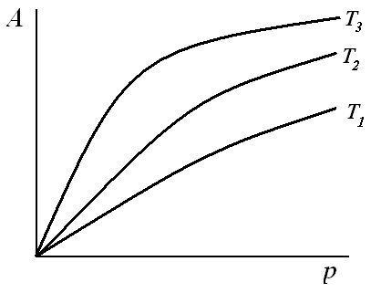
Посмотрим, какую форму примет уравнение при крайних значениях поверхностной концентрации адсорбированного вещества.
В области малых концентраций, т.е. при малых давлениях, КР >1, и единицей в знаменателе можно пренебречь:
т.е. величина адсорбции стремится к пределу, при котором она уже практически не зависит от давления (участок 3 изотермы адсорбции). В промежуточной области (участок 2) зависимость адсорбции от давления описывается самим уравнением (2.10).
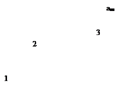
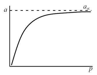
Рис. 2.5. Три участка изотермы адсорбции Ленгмюра
Таким образом, по модели Ленгмюра, вначале адсорбция растет пропорционально давлению газа, затем, по мере заполнения мест на поверхности, этот рост замедляется и, наконец, при достаточно высоких давлениях рост адсорбции практически прекращается, так как покрытие поверхности становится весьма близким к монослойному. Необходимо подчеркнуть, однако, что по этой модели завершение образования монослоя происходит лишь при бесконечно высоком давлении. Форма изотермы адсорбции, предсказываемая уравнением Ленгмюра, экспериментально наблюдается в случае химической адсорбции на однородных поверхностях. Для физической адсорбции такое соответствие наблюдается только в начальной области изотермы. При больших заполнениях не получается предсказываемого теорией приближения к насыщению и изотерма продолжает подъем с ростом давления, причем она становится даже более крутой.
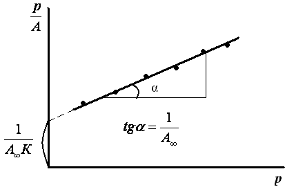
Для удобной проверки приложимости уравнения Ленгмюра к экспериментальным данным преобразуем его в линейную форму. Разделим обе части уравнения (2.10) на Р:
 . (2.13)
Перевернем дроби по обе части равенства:
 . (2.14)
Если по оси абсцисс откладывать Р, а на оси ординат Р/а, то в случае выполнимости уравнения Ленгмюра экспериментальные точки должны укладываться на прямую. Начальной ординатой будет 1/(аm∙К), тангенсом угла наклона прямой 1/аm. Из того и другого выражения легко вычислить обе константы am и К. Пример такого построения показан на рис. 2.6, где экспериментальные точки для адсорбции бензола на графитированной саже, в соответствии с указанными ранее, легли па прямую только в области малых давлений (до Р/Р0 =0.1).
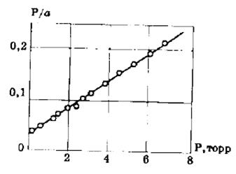
Рис. 2.6. Изотерма адсорбции бензола при 20 о С на графитированной саже в координатах линейной формы уравнения Ленгмюра
Имеется немало примеров, когда уравнение Ленгмюра не выполняется. Объясняется это тем, что не оправдываются оба допущения теории об однородности поверхности и отсутствии взаимодействия молекул, особенно первое из них. Тот факт, что имеются случаи адсорбции на реальных неоднородных поверхностях, когда уравнение Ленгмюра все же удовлетворительно описывает экспериментальные данные, Брунауер объясняет тем, что в некотором интервале адсорбция происходит не на всей поверхности адсорбента, а только на части ее, именно на местах с примерно одинаковой теплотой адсорбции. Тогда в этом интервале уравнение Ленгмюра будет справедливо. После того, как эти места заполнены, начинает заполняться следующая серия мест с меньшей теплотой адсорбции. Поэтому для совокупности всех мест поверхности уравнение Ленгмюра может быть непригодно, а для части этих мест — справедливо. Отсюда, выполнимость его для разных адсорбентов зависит от соотношения участков с разной теплотой адсорбции.
Константы уравнения (2.10) K и am могут быть определены графическим способом (рис. 2.7). Для этого уравнение Ленгмюра приводят к следующему линейному виду, разделив единицу на уравнение (2.10):
 (2.15)
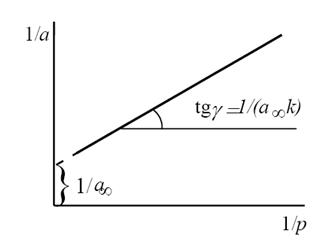
Рис. 2.7. Линейная форма уравнения изотермы Ленгмюра (a∞=am)
Зная емкость монослоя, можно определить удельную поверхность адсорбента Sуд (м 2 /г или см 2 /г) если известна площадь ω, занимаемая частицей в плотном адсорбционном слое (площадь, занимаемая одной молекулой азота в адсорбционном слое ω = 0.162 нм 2 ):
 , (16)
где аm — емкость монослоя — это количество адсорбата, которое может разместиться в полностью заполненном адсорбционном слое толщиной в 1 молекулу — монослое – на поверхности единицы массы (1г) твердого тела; ω — средняя площадь, занимаемая молекулой адсорбата в заполненном монослое, NA — число Авогадро (6,022·10 23 молекул/моль); VM — молярный объем адсорбата (газа) (VM = 22,41 л/моль=22,41∙10 -3 м 3 /моль).
Уравнение Ленгмюра можно использовать только при адсорбции в мономолекулярном слое. Это условие выполняется при хемосорбции, физической адсорбции газов при меньшем давлении и температуре выше критической.
Однако в большинстве случаев мономолекулярный адсорбционный слой не компенсирует полностью избыточную поверхностную энергию и поэтому остается возможность влияния поверхностных сил на второй и т.д. адсорбционные слои. Это реализуется в том случае, когда газы и пары адсорбируются при температуре ниже критической, т.е. образуются полимолекулярные слои на поверхности адсорбента, что можно представить как вынужденную конденсацию В этом случае используют уравнение БЭТ (Брунауер –Эммет — Теллер).
Пример 2.1. При адсорбции азота на активированном угле при 220К получены следующие данные:
Р, Па 5310 9800 18000 33000 70000
a, cм 3 /г 7 14 23 32 51
Плотность газообразного азота ρ=1,2506 кг/м 3 . Площадь, занимаемая одной молекулой азота в насыщенном монослое, составляет ω = 0.162 нм 2 . VM — молярный объем адсорбата (газа) (VM = 22,41 л/моль=22,41∙10 -3 м 3 /моль).
Постройте изотерму адсорбции в линейных координатах. Графически определите константы аm и К уравнения Ленгмюра, пользуясь которыми, постройте изотерму Ленгмюра. Определите удельную поверхность активированного угля Sуд.
Решение. Линейная форма уравнения Ленгмюра выражается (2.15):
 .
.
Определим 1/аm и 1/ р:
(1/р)·10 -3 , Па 0,1883 0,1020 0,0556 0,0303 0,0143
1/а·, см 3 /г 0,143 0,071 0,043 0,031 0,020
Строим график зависимости 1/а=f(1/р)∙10 -3 (рис.2.8). По графику находим 1/аm как отрезок, отсекаемый прямой на оси ординат, для чего необходимо продлить полученную прямую до пересечения с осью ординат.
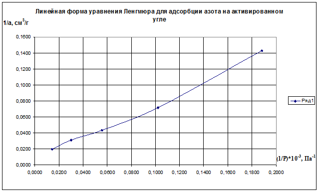
Рис.2.8. Линейная форма уравнения Ленгмюра для адсорбции азота на активированном угле
Уравнение прямой y=a+bx, имеет следующее формульное выражение:
Это выражение может быть определено с помощью регрессионного анализа в Microsoft Excel (встроенного пакета Анализ данных — Регрессия по значениям 1/аm и 1/ р).
Из уравнения получим 1/am=0,00698 г/см 3 .
Откуда получим: am=143,35 см 3 /г.
Далее находят тангенс угла наклона прямой к оси абсцисс tgα=1/(am∙K) по графику (или по уравнению регрессии). tgα=0,70099. Тогда, зная значения am и tgα, можно определить K=9,95 кг/м 3 .
Теперь, зная константы аm и К уравнения Ленгмюра, построим изотерму Ленгмюра, для чего рассчитаем по формуле (2.10) значения а для различных значений Р и получим:
Р, Па 5310 9800 18000 33000 70000
a, cм 3 /г 140,69 141,90 142,56 142,92 143,15
По данным значениям построим изотерму Ленгмюра а=f(P), представлена на рис.2.9.
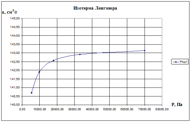
Рис. 2.9. Изотерма Ленгмюра а=f(P)
По формуле (2.16) рассчитаем удельную поверхность активированного угля: 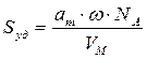 и получим Sуд=624,05 м 2 /г.
В случае, когда известна плотность вещества (адсорбента) ρ и молярная масса M, а не известен VM — молярный объем адсорбата удельную поверхность вещества (активированного угля) находят по формуле:
где am выражают в моль/кг.
Для азота М= 0,0280 кг/моль, ρ=1,2506 кг/м 3 .
Из расчетов видно, что два способа расчета Sуд дают почти одинаковые результаты.
Пример 2.2. Удельная поверхность непористой сажи равна 73,7м 2 /кг. Рассчитайте площадь, занимаемую молекулой бензола в плотном монослое, исходя из данных об адсорбции бензола на этом адсорбенте при 293 К.
Р, Па 1,03 1,29 1,74 2,50 6,67
а∙10 2 , моль/кг 1,57 1,94 2,55 3,51 7,58
Предполагается, что изотерма адсорбции описывается уравнением Ленгмюра.
Решение. Используем линейную форму записи уравнения Ленгмюра, заданную формулой (2.14):

Рассчитываем значения Р/а:
(Р/а)∙10 -2 , Па∙кг/моль 0,656 0,668 0,68 0,712 0,879
Р, Па 1,03 1,29 1,74 2,50 6,67
По этим данным строим график в координатах уравнения Ленгмюра в линейной форме P/a=f(P).
Из графика находим аm= Р/(Р/а) = 25,2∙10 -2 моль/кг.
Удельная поверхность адсорбента связана с емкостью слоя аm, выраженного в моль/кг, соотношением: Sуд=am∙ω∙NA (2.18)
Площадь, занимаемая молекулой бензола в плотном монослое, равна
ω = Sуд/(am NA) ==73,7 10 3 /(6,02 10 23 ∙25,210 -2 )=0,49∙10 -18 м 2 =0,49 нм 2 .
http://www.sites.google.com/site/kolloidnaahimia/adsorbcia-svistat-vseh-na-poverhnost/teoria-monomolekularnoj-adsorbcii-lengmura
http://helpiks.org/8-21027.html
Расчет констант уравнения Лэнгмюра
Константы
(К
и А∞)
уравнения Лэнгмюра рассчитывают
графическим способом, для этого уравнение
(1) приводят к линейному виду: y=a+bx.
![]()
. (2)
Строят изотерму
адсорбции в координатах линейной формы
уравнения Лэнгмюра (рис.2):
|
Рис.2. |
Экстраполяция
Тангенс угла
или |
Зная
величину
![]()
,
можно рассчитать удельную поверхность
адсорбента:
![]()
, (6)
где
S0 –
площадь, занимаемая одной молекулой
адсорбата, NA
– число Авогадро.
Представления,
развитые Лэнгмюром, в значительной
степени идеализируют и упрощают
действительную картину адсорбции. На
самом деле поверхность большинства
адсорбентов энергетически неоднородна,
между молекулами адсорбата имеют место
«боковые» взаимодействия.
|
Рис. |
При
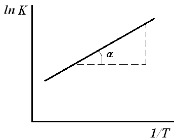
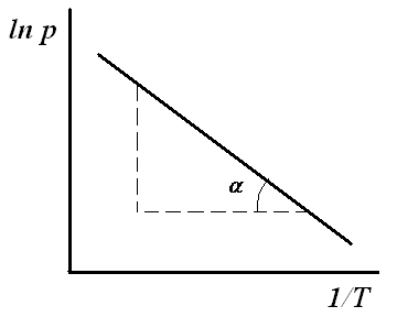
Константа
(7) |
Установив
экспериментальную зависимость константы
адсорбционного равновесия К
от температуры, можно определить
энтальпию адсорбции (интегральную
теплоту адсорбции).
Интегральная
теплота адсорбции характеризует
интенсивность взаимодействия адсорбента
с адсорбатом (газом или паром), она
отрицательна, что указывает на выделение
теплоты в процессе адсорбции и не зависит
от степени заполнения адсорбента газом.
Уравнение
(7) применяют для определения интегральной
теплоты адсорбции графическим способом,
для этого уравнение (7) интегрируют
(неопределенный интеграл):
![]()
, (8)
где
В ─ постоянная
интегрирования.
|
Рис.4. |
Интегральную
(9) |
Аналитический
способ расчета интегральной теплоты
адсорбции основан на уравнении:
![]()
. (10)
Каждой
степени заполнения поверхности адсорбента
соответствует некоторая дифференциальная
теплота адсорбции qA.
Дифференциальная изостерическая (A
= const)
теплота адсорбции всегда положительна
и уменьшается по мере роста степени
заполнения адсорбатом поверхности
адсорбента. Если значения qA
невелики (10 – 40 кДж/моль), то можно
говорить о физической адсорбции газов,
обусловленной физическими силами. Если
рассчитанные значения qA
находятся в пределах 40 – 400 кДж/моль, то
в этом случае адсорбция обусловлена
химическими силами (хемосорбция).
Для
расчета qA
строят изостеры адсорбции (зависимости
р
от Т)
при разных температурах (A
= const).
Для построения изостер адсорбции
проводят к изотермам адсорбции линии,
параллельные оси абсцисс. Графически
находят значения р
и Т
при разных А.
|
Рис.5. обратной |
Дифференциальную (рис.5) по уравнению:
(11) |
Аналитический
способ расчета дифференциальной теплоты
адсорбции основан на уравнении:
![]()
. (12)
Соседние файлы в предмете [НЕСОРТИРОВАННОЕ]
- #
- #
- #
- #
- #
- #
- #
- #
- #
- #
- #
the equilibrium adsorption constant and the corresponding free energy of adsorption were also calculated taking into account that the Langmuir model gives an average free energy that is independent of the solution concentration (∼ –34 kJ mol−1).
From: Handbook of Surfaces and Interfaces of Materials, 2001
The Properties of Water and their Role in Colloidal and Biological Systems
Carel Jan van Oss, in Interface Science and Technology, 2008
3.6 Importance of using the value for pre-hysteresis Keqt→0
Using the correct value for the equilibrium adsorption constant, Keq, is important, because it is the basis for deriving the value of ΔG1w2(mic); see Eq. (13.1), in Sub-section 2.2, above. Together with the kinetic adsorption rate constant, ka, knowledge of the accurate value of Keq (in the form of Keqt→0) is also a prerequisite for obtaining a reliable value for the kinetic desorption rate constant, kd; see Sub-section 4.4.5, below. (For the determination of ka, see Sub-section 4.3, below.)
It should be noted, meanwhile, that there is no need to designate Keqt→0 as “Keq(mic)” because there can be no “Keq(mac)” that could be linked to a ΔG1w2(mac) because the latter is generally repulsive and there is no actual attractive bond for which one might be able to express an equilibrium adsorption constant as “Keq(mac).” Thus, Keqt→0 is the equilibrium binding constant pertaining exclusively to microscopic-scale adsorption (here of HSA) and hence is only connected to ΔG1w2(mic); see Eq. (13.1).
Read full chapter
URL:
https://www.sciencedirect.com/science/article/pii/S1573428508002135
Characterization of Porous Solids VI
O. Šolcová, P. Schneider, in Studies in Surface Science and Catalysis, 2002
3.3 Tracer adsorption
The tracer adsorption parameter, δo, includes tracer adsorption equilibrium constant KT; δo = γ(1 + KT), and γ = β(1-α)/α. β is the pellet porosity and α is the column void fraction (interstitial void volume/column volume). Thus, γ, is the pore volume per unit interstitial volume. For an inert tracer KT = 0 and δo = γ. Parameters δo were determined from the difference of first peak moments for two column lengths. Thus, only tdif and tc were searched by the time-domain matching; these parameters are not correlated. From our experience the simplex algorithm [23] for minimization of the sum of squared differences between the calculated and experimental SPSC responses proved to be sufficiently rapid and stable.
Read full chapter
URL:
https://www.sciencedirect.com/science/article/pii/S0167299102801707
Reaction Kinetics and the Development of Catalytic Processes
D. Casanave, … M. Forissier, in Studies in Surface Science and Catalysis, 1999
Nomenclature
-
dp: pore diameter
-
F: objective function
-
J: jacobian matrix
-
KiC4 : adsorption equilibrium constant of isobutane (atm−1)
-
KiC4= : adsorption equilibrium constant of isobutene (atm−1)
-
KH : adsorption equilibrium constant of hydrogen (atm−1)m: mass of catalyst (g)
-
N: correlation matrix
-
PH2: partial pressure of hydrogen (atm)
-
PiC4: partial pressure of isobutane (atm)
-
PiC4=: partial pressure of isobutene (atm)
-
Qs: stream volumetric rater: rate of reaction (μmol.s−1.g−1)riC4=: rate of isobutene production (μmol.s−1.g−1)riC4: rate of isobutane production (μmol.s−1.g−1)s: standard deviation
-
T: reaction temperature (K)
-
V: variance-covariance matrix
Read full chapter
URL:
https://www.sciencedirect.com/science/article/pii/S0167299199801682
Adsorption and its Applications in Industry and Environmental Protection
M.S. Ray, in Studies in Surface Science and Catalysis, 1999
1987
Aharoni, C., Adsorption by nonhomogeneous porous solids: Effect of adsorption energy gradient on surface flow, AIChE J., 33(2), 303-306(1987).
Allen, S.J., Equilibrium adsorption isotherms for peat, Fuel, 66(9), 1171-1175 (1987).
Altshuller, D., et al., Analysis of countercurrent adsorber. Chem. Eng. Commun.. 52, 311-330 (1987).
Aracil, J., Use of factorial design of experiments in the determination of adsorption equilibrium constants (methyl iodide on charcoals), J. Chem. Technol. Biotechnol., 38(3), 143-152 (1987).
Burganos, V.N., and Sotirchos, S.V., Diffusion in pore networks: Effective medium theory and smooth field approximation, AIChE J., 33(10), 1678-1689 (1987).
Chen, T.L., and Hsu, J.T., Prediction of breakthrough curves by fast Fourier transform method, AIChE J., 33(8), 1387-1390(1987).
Davis, M.M., and LeVan, M.D., Equilibrium theory for complete adiabatic adsorption cycles, AIChE J., 33(3), 470-479(1987).
Jaroniec, M., and Madey, R., Gas adsorption on structurally heterogeneous microporous solids, Sep. Sci. Technol., 22(12), 2367-2380 (1987).
Kapoor, A., and Yang, R.T., Roll-up in fixed-bed multicomponent adsorption under pore-diffusion limitation, AIChE J., 33(7), 1215-1217(1987).
Mansour, A.R., Comparison of equilibrium and nonequilibrium models in simulation of multicomponent sorption processes, Sep. Sci. Technol., 22(4), 1219-1234 (1987).
Marutovsky, R.M., and Bulow, M., Sorption kinetics of multicomponent gaseous and liquid mixtures on porous sorbents (review paper), Gas Sep. Purif., 1(2), 66-76 (1987).
Talu, O., and Kabel, R.L., Isosteric heat of adsorption and vacancy solution model, AIChE J., 33(3), 510-514 (1987).
Tine, C.B.D., Single pellet model application to a two component fixed bed adsorber, Chem. Eng. Res. Des., 65(2), 199-206(1987).
Wankat, P.C., Intensification of sorption processes, Ind. Eng. Chem. Res., 26(8), 1579-1586 (1987).
Wittkopf, H., and Brauer, P., Statistical thermodynamic calculations for adsorption data of gases: Two-phase approach, Adsorpt. Sci. Technol., 4(4), 251-274 (1987).
Read full chapter
URL:
https://www.sciencedirect.com/science/article/pii/S0167299199805783
Surface Complexation Modelling
D.A. Kulik, in Interface Science and Technology, 2006
6.1. Three-term temperature extrapolations
In a moderate temperature interval (from 0 to 200 °C) under the saturated vapor pressure, the expression of the standard-state equilibrium adsorption constant KS as a function of temperature requires knowledge of standard ΔrHo298 (enthalpy) or ΔrSo298 (entropy) and ΔrCpo298 (heat capacity at constant pressure) effects of the reaction at reference To = 298.15 K. A set of such relatively simple so-called “three-term” extrapolations of 2-pK reactions (in TL GEM SCM) has been shown to describe well the surface charge on rutile from 25 to 250 − 290 °C [55]. Three-term extrapolations are usually expressed in the form
(117)ΔrGTo=ΔrGToo−(T−To)ΔrSToo+(T−To−TlnTTo)ΔrCpToo
where ΔrGTo=−ln(10)·RTlog10KT. Eq. (117) corresponds to the expression
(118)log10KT=a+bT+clnT
where the coefficients a, b, and c involve entropy, enthalpy, and heat capacity terms at To = 298.15 K:
(119)a=ΔrSToo−ΔrCpToo(1+lnTo)ln10·R; b=−ΔrHToo−ToΔrCpTooln10·R; c=ΔrCpTooln10·R
Setting ΔrCpToo=0 reduces Eq. (117) – (119) to the two-term (so-called Van’t Hoff) temperature extrapolation. Setting ΔrCpToo=1 and ΔrSToo=0 results in a one-term extrapolation with ΔrHTo=ΔrGToo and log10KT=ToTlog10KTo. Setting instead ΔrCpToo=0 and ΔrHToo=0 leads to another one-term extrapolation with constant log10KT = log10 KTo [106, 107]. One-term extrapolations may be very helpful when no experimental data for elevated temperatures exist.
Once the temperature correction is done and the values KT or ΔrGTo obtained, the molar Gibbs energy function of a surface species goT can be calculated from the reaction stoichiometry and from Gibbs energies of other involved species, corrected to the same temperature of interest. For aqueous species, gases and solids, the methods of temperature corrections are well known, described in textbooks [31, 108], and implemented in computer codes [109]. The necessary data (standard molar entropies, heat capacities etc.) are available from chemical thermodynamic data bases[76, 77, 110]. Therefore, the problem of temperature correction and extrapolation of goT for surface complexes is actually the problem of temperature correction of ΔrGoT or KT values for the adsorption reactions.
The three-term extrapolation, with non-zero a, b, and c terms, should be applied to reactions with all ionic charged species on one side, like ≡OH0 ↔ =O− + H+(aq) (analog of the water dissociation reaction), which involve large solvation and electrostriction energetic effects manifested in significant ΔrCpo, ΔrSo and ΔrHo values. The range of applicability of three-term extrapolations is actually limited because ΔrCpo is not constant over large temeperature intervals, where more sophisticated (e.g. 5-term) extrapolations are needed. Fortunately, reactions can often be re-formulated into the “isocoulombic” and “isoelectric” forms, where large energetic effects (almost) cancel out [106].
Read full chapter
URL:
https://www.sciencedirect.com/science/article/pii/S1573428506800517
FUELS – HYDROGEN PRODUCTION | Gas Cleaning: Pressure Swing Adsorption
S.D. Sharma, in Encyclopedia of Electrochemical Power Sources, 2009
Semianalytical Approach
In this approach, a set of partial differential equations are derived to represent the dynamic variation of concentrations of various components, temperature, and pressure at various points in the bed. Most of the models developed so far are two-dimensional (time t and bed height z) models with or without inclusion of axial dispersion effects and gradients. Usually, the radial dispersion is not considered in the modeling approach because of the complexity of handling three dimensions (time t, height z, and radius r) and the possibility of insignificant gain over the results obtained from a two-dimensional model.
The partial differential equations are derived from the mass, energy, and momentum balance across a small grid within the adsorbent bed. The parameters such as axial dispersion coefficient, adsorption equilibrium constant, mass transfer rate, thermal diffusivity, and bed permeability are experimentally determined or estimated quantities; therefore, this approach of design and optimization could be called semianalytical approach. The generic form of the mass, energy, and momentum balance is shown as eqns [1]–[3].
-
Dynamic mass balance:
[1]−[kgmole/s ofadsorbate species‘i’axially dispersed]+[kgmole/s of adsorbatespecies‘i’changed withthe bed depth]+[kgmole/s of adsorbatespecies‘i’changed alongthe axis with time]+[kgmole/s separationof species‘i’in theadsorbent bed]=0
-
Dynamic heat balance:
[2]−[kJs-1heat transfer due tothermal conductivityof adsorbent bed along theflow direction or axis]+[kJs−1heat transfer dueto flow of gas throughthe adsorbent bed]+[kJs−1heat tranfer tothe gas in the voidand adsorbent in thebed]+[kJs−1heat transferfrom gas in the bedto vessel wall]−[kJ s−1heat produceddue to adsorption inthe bed]=0
-
Dynamic momentum balance:
[3]−[kgfs−1pressure forceappiled at theinlet of adsorber]+[kgfs−1pressure forcerecovered at theoutlet of adsorber]+[kgfs−1pressure forceloss due to adsorptionon some mass of gas]+[kgfs−1pressure lossdue to friction inthe bed]+[kgfs−1pressure lossdue to gravity forces]=0
-
Although a dynamic equation could be written for the momentum balance and prediction of pressure drop across the bed, Darcy’s or Ergun’s equation seems to predict the variation of pressure drop across the bed. Ergun’s equation is a modified form of Darcy’s equation and it contains an additional term that includes molar density and molecular weight of the bulk gas to incorporate the effect of variation in bulk gas composition.
Read full chapter
URL:
https://www.sciencedirect.com/science/article/pii/B9780444527455003075
Membrane Gas Separation
Endre Nagy, in Basic Equations of Mass Transport Through a Membrane Layer (Second Edition), 2019
18.4.2.1 Langmuir Isotherm
The Langmuir isotherm comprises monolayer adsorption, no interaction between the adsorbed molecules and adsorbed molecules, adsorbed molecules are immobile, and adsorbed and desorbed molecules are in equilibrium (Fig. 18.1 illustrates this adsorption isotherm, which tends to give an upper value as a function of pressure; this limit value means that the interface is fully occupied by the monolayer adsorption):
(18.30)qi=qi,satbipi1+bipi
where bi is the adsorption equilibrium constant of component i (1/Pa), qi,sat is the saturation loading in the inorganic membrane of component i (mol/kg), and q is the loading of component i in the membrane (mol/kg). Eq. (18.30) can be given in linearized form for determination of the parameters of the isotherm as:
(18.31)piqi=1biqi,sat+piqi,sat.
By means of the slope and the intercept point of pi/qi versus the pi function, the parameters of bi and qi,sat can be determined. The adsorption isotherm in the case of a binary mixture, assuming that the sorption process of the components is independent from each other, is (pi + pj = po, where po is the total pressure) (Kapteijn et al., 2000; Van den Bergh et al., 2008):
(18.32)qi=qi,satbipi1+bipi+qj,satbjpj1+bjpj
and:
(18.33)bi=bi,oexp(−ΔHi,adsnRT)
where ΔHi is the adsorption enthalpy (J/mol), bi,o is the preexponential of adsorption equilibrium constant (1/Pa), and n is the adsorption site n. The extension of the unary isotherm to the binary system for the competitive sorption process gives (Ahmadpour et al., 1998):
(18.34)qi=qi,satbipi1+b1p1+b2p2i=1,2.
For a multicomponent system (O’Brien and Myers, 1984):
(18.35)qi=qi,satbipi1+∑j=1Nbjpj.
Read full chapter
URL:
https://www.sciencedirect.com/science/article/pii/B9780128137222000182
Energy Materials
Mashallah Rezakazemi, Zhien Zhang, in Comprehensive Energy Systems, 2018
2.29.4.5.1 Langmuir isotherm
The Langmuir isotherm model is based on the assumptions that the adsorption process occurs at particular homogeneous sites on the surface of the adsorbent [62]. Moreover, this model is also based on the assumptions that when a molecule is adsorbed onto a site, other molecules are not able to adsorb at that site. When the adsorption of organosulfur from fuels obeys the Langmuir isotherm, the theoretical relationship between the volume of organosulfur in the fuels and the volume of organosulfur attached on the surface of adsorbent at equilibrium conditions, the concentration of adsorbed organosulfur can also be described as follows [63,64]:
(12)q=KqmCe1+KCe
where q and K are the concentration of adsorbed organosulfur and the adsorption equilibrium constant, respectively. qm and Ce are the maximum adsorption capacity and the concentration of the organosulfur compound in fuel, respectively [63,64].
The Eq. (12) can be rearranged into a linear form as shown below:
(13)Ceq=1Kqm+Ceqm
Since the concentration of the organosulfur compound in fuels is relatively low (i.e., Ce≪1), therefore, the reaction rate can be considered be first order. A graph of Ce/q against Ce would yield a straight line, which determines the adsorption capacity term, qm, from the slope (1/qm) as well as the adsorption equilibrium constant, K, from the intercept (1/qmK). The adsorption terms qm and K relatively specify the tendency of the adsorbate to the surface of nanoadsorbent and explains the physical, chemical, and dynamic characteristic of a nanoadsorbent [63,64].
The separation factor is useful to determine the value of the dimensionless adsorption constant as follows [68].
(14)r=11+KC0
The value of r shows the type of the adsorption isotherm. With increasing temperature, the value of r decreases indicating the adsorption process is desirable at high temperatures [66]. In Table 6, the values of r and the relevant types of adsorption isotherm are given.
Table 6. Total sulfur concentration of four JP-8 from Fort Belvoir, Virginia
| Values of r | Type of adsorption isotherm |
|---|---|
| r>0 | Unfavorable |
| r=1 | Linear |
| 0<r<1 | Favorable |
| r=0 | Irreversible |
Source: Reproduced with permission from LeeIC, Ubanyionwu HC. Determination of sulfur contaminants in military jet fuels, Fuel 2008;87:312–18. Available from: http://dx.doi.org/10.1016/j.fuel.2007.05.010.
The Brunauer–Emmett–Teller (BET) model is a developed model of the Langmuir isotherm that considers the multilayers of coverage that are not allowed in the Langmuir isotherm. The BET expression is illustrated in Eq. (3). The BET expression is extensively used to measure the surface area of adsorbent surfaces by calculating the physical adsorption of nitrogen in terms of pressure [63,64].
(15)1ν[(P0P)−1]=c−1vmc(P0P)+1vmc
where P and P0 are equilibrium pressure and saturation pressure, respectively. Here, v and vm are adsorbed gas quantity and monolayer adsorbed gas quantity, respectively [63,64].
Read full chapter
URL:
https://www.sciencedirect.com/science/article/pii/B9780128095973002637
Inorganic Photochemistry
B. Ohtani, in Advances in Inorganic Chemistry, 2011
B Langmuir–Hinshelwood Mechanism
The term “Langmuir–Hinshelwood mechanism” has often been used in discussion of the mechanism of photocatalytic reaction in suspension systems, but, as far as the author knows, there has been no definition given for the Langmuir–Hinshelwood (L–H) mechanism in photocatalytic reactions. In most cases, authors have claimed that a photocatalytic reaction proceeds via the L–H mechanism when a linear reciprocal relation is observed between the reaction rate and the concentration of reaction substrate in a solution. These experimental results seem to be consistent with the following equation:
(3)r=ksKCKC+1,
where r, k, K, s, and C are rate of the reaction, rate constant of the reaction of the surface-adsorbed substrate with e– (h+), adsorption equilibrium constant, limiting amount of surface adsorption, and concentration of substrate in the bulk at equilibrium, respectively (21), when the substrate is adsorbed by a photocatalyst obeying a Langmuir isotherm and the adsorption equilibrium is maintained during the photocatalytic reaction, that is, the rate of adsorption is faster than that of the reaction with electrons or holes (Section IV.A). Such a situation is often called “light-intensity limited,” that is, photoabsorption is the rate-determining step (22). Several methods for linearization of Eq. (3) have been reported, but two kinds of plots are often employed for analysis. As shown in Fig. 7, the most popular one is a plot of reciprocal rate against reciprocal concentration, and another one is a plot of ratio of concentration to rate against concentration. Both plots give ideally the same values of parameters, ks and K, while the former plot reflects mainly lower-concentration data with probable relatively large experimental error.

Fig. 7. Simulation of linearized plots for kinetics governed by surface concentration of substrates adsorbed on the photocatalyst surface in a Langmuirian fashion, where r, C, k, K, and S are rate of reaction (mol s− 1), concentration of a substrate (mol L− 1), rate constant (10− 4 s− 1), adsorption equilibrium constant (5 L mol− 1), and saturated amount of adsorption (2 × 10− 3 mol).
The original meaning of the term “Langmuir–Hinshelwood mechanism” in the field of catalysis is, to the author’s knowledge, a reaction of two kinds of molecules proceeding on a surface in which both molecules are adsorbed at the same surface adsorption sites with the surface reaction being the rate-determining step (in the original meaning of “rate-determining step”). Of course, the general rate equation for the L–H mechanism (not shown here) includes two sets of parameters for two kinds of molecules, and when one set of parameters is neglected, the equation is for a monomolecular reaction, similar to the photocatalytic reaction of a substrate adsorbed in Langmuirian fashion. However, at least in the field of catalysis, the term L–H mechanism is rarely used for such monomolecular surface reactions, since the L–H mechanism has been discussed for a bimolecular surface reaction by comparing with the Rideal-Eley mechanism, in which a surface-adsorbed molecule reacts with a molecule coming from the bulk.
Even if the L–H mechanism is defined as the reaction of a surface-adsorbed substrate obeying a Langmuir isotherm governing the overall rate, the frequently reported experimental evidence, a reciprocal linear relation between concentration of the substrate in solution and rate of photocatalytic reaction is not always proof of this mechanism. From the linear plot, two parameters are calculated (23). One (often shown as “k,” not as “ks”) is a limiting rate of the reaction at the infinite concentration giving maximum adsorption, that is, ks, and the other is the adsorption equilibrium constant, K. The former parameter is a product of rate constant and adsorption capacity of a photocatalyst and this may be a photocatalytic activity. The latter parameter shows the strength of adsorption and must be the same as that estimated from an adsorption isotherm measured in the dark. If kinetically obtained K is different from that obtained in dark adsorption measurement, the L–H mechanism cannot be adopted. Therefore, dark adsorption measurement is always required. Finally, it should be noted also in this case that a linear relation fitting to a Langmuir-type adsorption isotherm and similarity of adsorption equilibrium constant evaluated using photocatalytic reaction rate and by dark adsorption experiments are only necessary conditions; the observed reaction rate is “consistent” with kinetics of a substrate undergoing Langmuir-type adsorption and does not exclude the possibility of other reaction kinetics (24).
Read full chapter
URL:
https://www.sciencedirect.com/science/article/pii/B9780123859044000019
Fundamentals of Reaction Kinetics
Shaofen LiProfessor, in Reaction Engineering, 2017
2.8.2 Differential Method
The differential method directly uses the reaction rate equation to determine kinetic parameters based on the reaction rate data measured at different conditions. Using Eq. (2.99) as an example, take the logarithm on both sides:
Based on experimental data, a straight line can be obtained when plotting ln rA against ln cA. The slope is α, and the intercept is ln k.
For Eq. (2.101a), it can be rearranged as:
(2.101c)pArA=1kpA+1kKA
Plot pA / rA against pA, the slope of the straight line obtained is 1/k, and the intercept is 1/kKA. Generally speaking, the graphic method is effective if the kinetic parameters are no more than two and the rate equation can be linearized.
Similar to the integration method, when there are more than two parameters in the rate equation, for the differential method it is not practical to use the graphic method for parameter estimation unless some special experimental design would allow for simplification. Therefore, for kinetic data analysis using either integration or differential methods the most commonly used and versatile approach is regression of experimental data based on statistic principle. Such an approach does not have a limit on the number of parameters, the format of the kinetic equations, or the experimental design, and is very versatile. Next we will discuss the fundamental principles of this approach.
Theoretically speaking, the number of experimental data required are equal to the number of parameters to be determined. For example, Eq. (2.101a) has two parameters, i.e., k and KA. If two reaction rates, rA1 and rA2, were measured experimentally at two partial pressures of A, pA1 and pA2. Using these two sets of data in Eq. (2.101a) we will get two equations of k and KA, and by solving these two equations we can determine k and KA. However, since it is unavoidable that there will be some experimental error, it is not reliable to determine two parameters based on just two sets of data. In reality, the number of experimental data sets must be more than the number of parameters to be determined. More experimental data would make parameter estimation more reliable. Therefore, there will be more equations than the number of parameters to be determined and the least square method can be used to determine the values of the parameters.
The fundamental principle for the least square method is to seek parameter values that will make the residual sum of square to be at minimum. The residual is the difference between experimental value η and the value predicted by the model ηˆ, and therefore the residual sum of square:
(2.102)Φ=∑i=1M(ηi−ηˆi)2=min
where M is the number of experiments, η is the physical value to be measured. For example, when the differential method is used for kinetic study, typically the reaction rate is measured. Under this situation Eq. (2.102) becomes:
(2.103)Φ=∑i=1M(ri−rˆi)2=min
Therefore the goal is to minimize the residual sum of square between the experimentally measured rate and the value calculated by the reaction rate equation. For Eq. (2.101a), the above equation becomes:
(2.104)Φ=∑i=1M(ri−kKApAi1+KApAi)2=min
where pAi is the partial pressure of component A for ith experiment, and ri is the measured reaction rate at this partial pressure. Now the residual sum of square Φ is a function of k and KA. What we need to do next is to find the values of k and KA to minimize Φ, and this can be achieved by using the extremum seeking method. Taking the derivative of Eq. (2.104) with respect to k and KA, and setting dΦ/dk=0 and dΦ /dKA=0, we will get two equations. By solving these two equations we will obtain k and KA. The same procedure can be used for more parameters. The only difference is the number of equations will increase.
Based on the procedure described above, to obtain parameters using the least square method we need to solve a group of equations as follows:
∂Φ∂ki=0,i=1,2,3,…,N
ki are the kinetic parameters and N is the number of kinetic parameters to be determined. This is a group of algebra equations. In most situations the kinetic equations are nonlinear, therefore this is a group of nonlinear algebra equations. As a result, this procedure is often called a nonlinear least square method or nonlinear regression.
Solving a group of nonlinear algebra equations is not easy, especially when there are many equations. If the rate equations can be transformed into a linear format, it will make the parameter estimation much easier mathematically. For example, Eq. (2.101a) can be rewritten in a linear format as Eq. (2.101c). If pA/rA=η, 1/k=α, and 1/(kKA)=β, Eq. (2.101a) can be expressed as:
(2.105)η=αpA+β
After transformation, the residual sum of square becomes:
Φ=∑i=1M(ηi−αpAi−β)2=min
Taking the derivative with respect to α and β and letting them equal zero, two linear algebra equations of α and β can be obtained, and then solved to get α and β. Based on the definition of α and β given above, k and KA can be calculated. Regression after linearization is called the linear regression method, or linear least square method. The obvious advantage of the linear least square method is a group of linear algebra equations needs to be solved, and solving linear algebra equations is a lot easier and simpler than solving nonlinear algebra equations. However, the transformation may introduce additional errors for parameter estimation. Parameter estimation is very rich in content, and here we can only give a brief introduction of its fundamental principles.
Example 2.9
For benzene hydrogenation on nickel catalyst, the reaction rate equation has already been derived in Example 2.7
rB=kpBpH0.51+KBpB
where pB and pH are the partial pressure of benzene and hydrogen, respectively; k is the rate constant and KB is the adsorption equilibrium constant of benzene. At 423K the reaction rates at various gas compositions were measured in the lab and the data are given in Table 2C. Please calculate the rate constant and benzene adsorption equilibrium constant.
Table 2C. Reaction Rate for Benzene Hydrogenation Reaction at 423K
| Partial Pressure pi×103 MPa | Reaction Rate rB×103/[mol/(g·h)] | ||
|---|---|---|---|
| Benzene | Hydrogen | Cyclohexane | |
| 2.13 | 93.0 | 4.29 | 18.1 |
| 2.42 | 85.5 | 11.50 | 19.0 |
| 3.81 | 78.0 | 17.20 | 27.0 |
| 5.02 | 86.8 | 7.65 | 30.9 |
| 5.80 | 79.6 | 13.90 | 35.2 |
| 13.9 | 84.0 | 1.92 | 42.4 |
| 10.7 | 80.6 | 7.47 | 39.6 |
| 9.58 | 89.3 | 1.93 | 40.8 |
| 9.02 | 88.1 | 2.78 | 36.5 |
| 7.95 | 86.9 | 4.24 | 35.7 |
| 6.46 | 86.3 | 6.48 | 33.8 |
| 4.73 | 92.4 | 4.6 | 30.4 |
| 4.01 | 92.5 | 2.34 | 29.7 |
| 3.30 | 92.2 | 3.20 | 26.3 |
Solution
First we transform the rate equation into linear form:
(A)pBpH0.5rB=1k+KBkpB
If we plot pBpH0.5rB against pB we will get a straight line, and the slope and intercept can be used to calculate k and KB. For convenience, let pBpH0.5rB=y, 1/k=b, and KBk=a, then Eq. (A) becomes:
(B)y=apB+b
Using the data given in Table 2C, the values of y can be calculated, as shown in Table 2D, and then plot y against pB, as shown in Fig. 2C. The slope of the straight line is 4.763 and the intercept is 0.0215, i.e.:
Table 2D. Relationship Between y and pB
| pB×103 | y×102 | pB2×106 | pBy×105 |
|---|---|---|---|
| 2.13 | 3.589 | 4.537 | 7.645 |
| 2.42 | 3.742 | 5.856 | 9.012 |
| 3.81 | 3.941 | 14.52 | 15.015 |
| 5.02 | 4.786 | 25.20 | 24.026 |
| 5.80 | 4.649 | 33.64 | 26.964 |
| 13.90 | 9.592 | 193.20 | 133.329 |
| 10.70 | 7.671 | 114.50 | 82.080 |
| 9.58 | 7.017 | 91.78 | 67.223 |
| 9.02 | 7.335 | 81.36 | 66.162 |
| 7.95 | 6.565 | 63.20 | 52.192 |
| 5.46 | 5.615 | 41.73 | 36.273 |
| 4.73 | 4.730 | 22.7 | 22.273 |
| 4.01 | 4.106 | 19.08 | 16.465 |
| 3.30 | 3.810 | 10.89 | 12.573 |
| Σ 0.08883 | 0.7713 | 7.189×10⁻⁴ | 5.713×10⁻³ |
Unit: pi: MPa, rB: mol/(g·h).

Figure 2C. Relationship between y and pB.
b=0.0215=1/k
k=46.51 mol/(g·h·MPa1.5)
a=4.763=KB/k
KB=4.763×46.51=221.51/MPa
For comparisons’ sake, a and b are estimated by using the least square method. By seeking the minimum of the residual sum of square the following bivariate linear regression equations can be obtained:
(C)a=∑MpB∑My−M∑MpBy(∑MpB)2−M∑MpB2
(D)b=1M[∑My−a∑MpB]
where M is the number of experimental data. In this example, M=14. In order to calculate a and b using Eqs. (C) and (D), pB2 and pBy need to be calculated, which are also shown in Table 2D. Then using Eqs. (C) and (D)
a=0.08883×0.7713−14×5.713×10−30.088832−14×7.189×1−4=5.2716
b=0.7713−5.2716×0.0888314=0.02166
Therefore
k=1/b=46.16 mol/(g·h·MPa1.5)
KB=ak=5.2716×46.17=243.41/MPa
We can see the values of k and KB calculated from these two approaches are very close. Generally speaking, the values obtained from the linear least square method are more accurate.
Example 2.10
For gas phase hydrogenation of benzene on nickel catalyst, the rate constant and benzene adsorption equilibrium constant are experimentally measured at different temperatures:
| T/K | 363 | 393 | 423 | 453 |
|---|---|---|---|---|
| k/[mol/(g·h·MPa1.5)] | 14.52 | 25.96 | 45.07 | 66.03 |
| KB/(1/MPa) | 1495 | 537.3 | 237.9 | 99.41 |
Please calculate reaction activation energy and heat of adsorption for benzene.
Solution
The temperature dependences of the reaction rate constant and benzene adsorption equilibrium constant on temperature are expressed below:
(A)k=Aexp(−ERT)
(B)KB=KB0exp(qBRT)
Take logarithm on both sides of Eqs. (A) and (B)
(C)ln(k)=ln(A)−E/(RT)
(D)ln(KB)=lnKB0+qB/(RT)
Plotting ln(k) and ln(KB) against 1/T will give straight lines and the slopes can be used to calculate activation and energy and heat of adsorption. Using the data given above, 1/T, ln(k), and ln(KB) can be calculated:
| 1/T×103 | 2.755 | 2.545 | 2.364 | 2.208 |
| lnk | −0.759 | −0.178 | 0.374 | 0.756 |
| lnKB | 5.02 | 3.99 | 3.18 | 2.31 |
The plots are shown in Fig. 2D. The solid line is ln(k) versus 1/T and the dashed line is ln(KB) versus 1/T, and the slope for these two lines are −2.84×10³ and 5.3×10³, respectively. From Eq. (C), the slope is –E/R, therefore:

Figure 2D. Dependence of ln(k) and ln(KB) on 1/T.
E=2.84×103×8.313=2.36×10⁴J/mol
From Eq. (D) we see the slope of the dashed line is qB/R, therefore:
qB=5.3×103×8.313=4.41×10⁴J/mol
Similarly, since both ln(k) and ln(KB) are linear functions of 1/T, the linear least square method can also be used to calculate E and qB, which usually gives more accurate results.
Read full chapter
URL:
https://www.sciencedirect.com/science/article/pii/B9780124104167000021