![]()
Загрузить PDF
![]()
Загрузить PDF
До появления калькуляторов студенты и преподаватели вычисляли квадратные корни вручную. Существует несколько способов вычисления квадратного корня числа вручную. Некоторые из них предлагают только приблизительное решение, другие дают точный ответ.
-

1
Разложите подкоренное число на множители, которые являются квадратными числами. В зависимости от подкоренного числа, вы получите приблизительный или точный ответ. Квадратные числа – числа, из которых можно извлечь целый квадратный корень. Множители – числа, которые при перемножении дают исходное число.[1]
Например, множителями числа 8 являются 2 и 4, так как 2 х 4 = 8, числа 25, 36, 49 являются квадратными числами, так как √25 = 5, √36 = 6, √49 = 7. Квадратные множители – это множители, которые являются квадратными числами. Сначала попытайтесь разложить подкоренное число на квадратные множители.- Например, вычислите квадратный корень из 400 (вручную). Сначала попытайтесь разложить 400 на квадратные множители. 400 кратно 100, то есть делится на 25 – это квадратное число. Разделив 400 на 25, вы получите 16. Число 16 также является квадратным числом. Таким образом, 400 можно разложить на квадратные множители 25 и 16, то есть 25 х 16 = 400.
- Записать это можно следующим образом: √400 = √(25 х 16).
-
2
Квадратные корень из произведения некоторых членов равен произведению квадратных корней из каждого члена, то есть √(а х b) = √a x √b.[2]
Воспользуйтесь этим правилом и извлеките квадратный корень из каждого квадратного множителя и перемножьте полученные результаты, чтобы найти ответ.- В нашем примере извлеките корень из 25 и из 16.
- √(25 х 16)
- √25 х √16
- 5 х 4 = 20
- В нашем примере извлеките корень из 25 и из 16.
-
3
Если подкоренное число не раскладывается на два квадратных множителя (а так происходит в большинстве случаев), вы не сможете найти точный ответ в виде целого числа. Но вы можете упростить задачу, разложив подкоренное число на квадратный множитель и обыкновенный множитель (число, из которого целый квадратный корень извлечь нельзя). Затем вы извлечете квадратный корень из квадратного множителя и будете извлекать корень из обыкновенного множителя.
- Например, вычислите квадратный корень из числа 147. Число 147 нельзя разложить на два квадратных множителя, но его можно разложить на следующие множители: 49 и 3. Решите задачу следующим образом:
- √147
- = √(49 х 3)
- = √49 х √3
- = 7√3
- Например, вычислите квадратный корень из числа 147. Число 147 нельзя разложить на два квадратных множителя, но его можно разложить на следующие множители: 49 и 3. Решите задачу следующим образом:
-
4
Если нужно, оцените значение корня. Теперь можно оценить значение корня (найти приблизительное значение), сравнив его со значениями корней квадратных чисел, находящихся ближе всего (с обеих сторон на числовой прямой) к подкоренному числу. Вы получите значение корня в виде десятичной дроби, которую необходимо умножить на число, стоящее за знаком корня.
- Вернемся к нашему примеру. Подкоренное число 3. Ближайшими к нему квадратными числами будут числа 1 (√1 = 1) и 4 (√4 = 2). Таким образом, значение √3 расположено между 1 и 2. Та как значение √3, вероятно, ближе к 2, чем к 1, то наша оценка: √3 = 1,7. Умножаем это значение на число у знака корня: 7 х 1,7 = 11,9. Если вы сделаете расчеты на калькуляторе, то получите 12,13, что довольно близко к нашему ответу.
- Этот метод также работает с большими числами. Например, рассмотрим √35. Подкоренное число 35. Ближайшими к нему квадратными числами будут числа 25 (√25 = 5) и 36 (√36 = 6). Таким образом, значение √35 расположено между 5 и 6. Так как значение √35 намного ближе к 6, чем к 5 (потому что 35 всего на 1 меньше 36), то можно заявить, что √35 немного меньше 6. Проверка на калькуляторе дает нам ответ 5,92 — мы были правы.
- Вернемся к нашему примеру. Подкоренное число 3. Ближайшими к нему квадратными числами будут числа 1 (√1 = 1) и 4 (√4 = 2). Таким образом, значение √3 расположено между 1 и 2. Та как значение √3, вероятно, ближе к 2, чем к 1, то наша оценка: √3 = 1,7. Умножаем это значение на число у знака корня: 7 х 1,7 = 11,9. Если вы сделаете расчеты на калькуляторе, то получите 12,13, что довольно близко к нашему ответу.
-
5
Еще один способ – разложите подкоренное число на простые множители. Простые множители – числа, которые делятся только на 1 и самих себя. Запишите простые множители в ряд и найдите пары одинаковых множителей. Такие множители можно вынести за знак корня.
- Например, вычислите квадратный корень из 45. Раскладываем подкоренное число на простые множители: 45 = 9 х 5, а 9 = 3 х 3. Таким образом, √45 = √(3 х 3 х 5). 3 можно вынести за знак корня: √45 = 3√5. Теперь можно оценить √5.
- Рассмотрим другой пример: √88.
- √88
- = √(2 х 44)
- = √ (2 х 4 х 11)
- = √ (2 х 2 х 2 х 11). Вы получили три множителя 2; возьмите пару из них и вынесите за знак корня.
- = 2√(2 х 11) = 2√2 х √11. Теперь можно оценить √2 и √11 и найти приблизительный ответ.
Реклама


При помощи деления в столбик
-
1
Этот метод включает процесс, аналогичный делению в столбик, и дает точный ответ. Сначала проведите вертикальную линию, делящую лист на две половины, а затем справа и немного ниже верхнего края листа к вертикальной линии пририсуйте горизонтальную линию. Теперь разделите подкоренное число на пары чисел, начиная с дробной части после запятой. Так, число 79520789182,47897 записывается как «7 95 20 78 91 82, 47 89 70».
- Для примера вычислим квадратный корень числа 780,14. Нарисуйте две линии (как показано на рисунке) и слева сверху напишите данное число в виде «7 80, 14». Это нормально, что первая слева цифра является непарной цифрой. Ответ (корень из данного числа) будете записывать справа сверху.
-
2
Для первой слева пары чисел (или одного числа) найдите наибольшее целое число n, квадрат которого меньше или равен рассматриваемой паре чисел (или одного числа). Другими словами, найдите квадратное число, которое расположено ближе всего к первой слева паре чисел (или одному числу), но меньше ее, и извлеките квадратный корень из этого квадратного числа; вы получите число n. Напишите найденное n сверху справа, а квадрат n запишите снизу справа.
- В нашем случае, первым слева числом будет число 7. Далее, 4 < 7, то есть 22 < 7 и n = 2. Напишите 2 сверху справа — это первая цифра в искомом квадратном корне. Напишите 2×2=4 справа снизу; вам понадобится это число для последующих вычислений.
-
3
Вычтите квадрат числа n, которое вы только что нашли, из первой слева пары чисел (или одного числа). Результат вычисления запишите под вычитаемым (квадратом числа n).
- В нашем примере вычтите 4 из 7 и получите 3.
-
4
Снесите вторую пару чисел и запишите ее около значения, полученного в предыдущем шаге. Затем удвойте число сверху справа и запишите полученный результат снизу справа с добавлением «_×_=».
- В нашем примере второй парой чисел является «80». Запишите «80» после 3. Затем, удвоенное число сверху справа дает 4. Запишите «4_×_=» снизу справа.
-
5
Заполните прочерки справа. Найдите такое наибольшее число на место прочерков справа (вместо прочерков нужно подставить одно и тоже число), чтобы результат умножения был меньше или равен текущему числу слева.
- В нашем случае, если вместо прочерков поставить число 8, то 48 х 8 = 384, что больше 380. Поэтому 8 — слишком большое число, а вот 7 подойдет. Напишите 7 вместо прочерков и получите: 47 х 7 = 329. Запишите 7 сверху справа — это вторая цифра в искомом квадратном корне числа 780,14.
-
6
Вычтите полученное число из текущего числа слева. Запишите результат из предыдущего шага под текущим числом слева, найдите разницу и запишите ее под вычитаемым.
- В нашем примере, вычтите 329 из 380, что равно 51.
-
7
Повторите шаг 4. Если сносимой парой чисел является дробная часть исходного числа, то поставьте разделитель (запятую) целой и дробной частей в искомом квадратном корне сверху справа. Слева снесите вниз следующую пару чисел. Удвойте число сверху справа и запишите полученный результат снизу справа с добавлением «_×_=».
- В нашем примере следующей сносимой парой чисел будет дробная часть числа 780.14, поэтому поставьте разделитель целой и дробной частей в искомом квадратном корне сверху справа. Снесите 14 и запишите снизу слева. Удвоенным числом сверху справа (27) будет 54, поэтому напишите «54_×_=» снизу справа.
-
8
Повторите шаги 5 и 6. Найдите такое наибольшее число на место прочерков справа (вместо прочерков нужно подставить одно и тоже число), чтобы результат умножения был меньше или равен текущему числу слева.
- В нашем примере 549 х 9 = 4941, что меньше текущего числа слева (5114). Напишите 9 сверху справа и вычтите результат умножения из текущего числа слева: 5114 — 4941 = 173.
-
9
Если для квадратного корня вам необходимо найти больше знаков после запятой, напишите пару нулей у текущего числа слева и повторяйте шаги 4, 5 и 6. Повторяйте шаги, до тех пор пока не получите нужную вам точность ответа (число знаков после запятой).
Реклама


Понимание процесса
-
1
Для усвоения данного метода представьте число, квадратный корень которого необходимо найти, как площадь квадрата S. В этом случае вы будете искать длину стороны L такого квадрата. Вычисляем такое значение L, при котором L² = S.
-
2
Задайте букву для каждой цифры в ответе. Обозначим через A первую цифру в значении L (искомый квадратный корень). B будет второй цифрой, C — третьей и так далее.
-
3
Задайте букву для каждой пары первых цифр. Обозначим через Sa первую пару цифр в значении S, через Sb — вторую пару цифр и так далее.
-
4
Уясните связь данного метода с делением в столбик. Как и в операции деления, где каждый раз нас интересует только одна следующая цифра делимого числа, при вычислении квадратного корня мы последовательно работаем с парой цифр (для получения одной следующей цифры в значении квадратного корня).
-
5
Рассмотрим первую пару цифр Sa числа S (Sa = 7 в нашем примере) и найдем ее квадратный корень. В этом случае первой цифрой A искомого значения квадратного корня будет такая цифра, квадрат которой меньше или равен Sa (то есть ищем такое A, при котором выполняется неравенство A² ≤ Sa < (A+1)²). В нашем примере, S1 = 7, и 2² ≤ 7 < 3²; таким образом A = 2.
- Допустим, что нужно разделить 88962 на 7; здесь первый шаг будет аналогичным: рассматриваем первую цифру делимого числа 88962 (8) и подбираем такое наибольшее число, которое при умножении на 7 дает значение меньшее или равное 8. То есть ищем такое число d, при котором верно неравенство: 7×d ≤ 8 < 7×(d+1). В этом случае d будет равно 1.
-
6
Мысленно представьте квадрат, площадь которого вам нужно вычислить. Вы ищите L, то есть длину стороны квадрата, площадь которого равна S. A, B, C — цифры в числе L. Записать можно иначе: 10А + B = L (для двузначного числа) или 100А + 10В + С = L (для трехзначного числа) и так далее.
- Пусть (10A+B)² = L² = S = 100A² + 2×10A×B + B². Запомните, что 10A+B — это такое число, у которого цифра B означает единицы, а цифра A — десятки. Например, если A=1 и B=2, то 10A+B равно числу 12.(10A+B)² — это площадь всего квадрата, 100A² — площадь большого внутреннего квадрата, B² — площадь малого внутреннего квадрата, 10A×B — площадь каждого из двух прямоугольников. Сложив площади описанных фигур, вы найдете площадь исходного квадрата.
-
7
Вычтите A² из Sa. Для учета множителя 100 снесите одну пару цифр (Sb) из S: вам нужно, чтобы «SaSb» было равным общей площади квадрата, и из нее вычтите 100A² (площадь большого квадрата). В результате получите число N1, стоящее слева в шаге 4 (N = 380 в нашем примере). N1 = 2×10A×B + B² (площадь двух прямоугольников плюс площадь малого квадрата).
-
8
Выражение N1 = 2×10A×B + B² можно записать как N1 = (2×10A + B) × B. В нашем примере вам известно значение N1 (=380) и A(=2) и необходимо вычислить B. Скорее всего, B не является целым числом, поэтому необходимо найти наибольшее целое B, удовлетворяющее условию: (2×10A + B) × B ≤ N1. При этом B+1 будет слишком большим, поэтому N1 < (2×10A + (B+1)) × (B+1).
-
9
Решите уравнение. Для решения умножьте A на 2, переведите результат в десятки (что эквивалентно умножению на 10), поместите B в положение единиц, и умножьте это число на B. Это число (2×10A + B) × B и это выражение абсолютно идентичны записи «N_×_=» (где N=2×A) сверху справа в шаге 4. А в шаге 5 вы находите наибольшее целое B, которое ставится на место прочерков и соответствует неравенству: (2×10A + B) × B ≤ N1.
-
10
Вычтите площадь (2×10A + B) × B из общей площади (слева в шаге 6). Так вы получите площадь S-(10A+B)², которая еще не учитывалась (и которая поможет вычислить следующие цифры).
-
11
Для вычисления следующей цифры C повторите процесс. Слева снесите следующую пару цифр (Sc) из S для получения N2 и найдите наибольшее C, удовлетворяющее условию (2×10×(10A+B)+C) × C ≤ N2 (что эквивалентно двукратному написанию числа из пары цифр «A B» с соответствующим «_×_=», и нахождению наибольшего числа, которое можно подставить вместо прочерков).
Реклама


Советы
- Перемещение десятичного разделителя при увеличении числа на 2 цифры (множитель 100), перемещает десятичный разделить на одну цифру в значении квадратного корня этого числа (множитель 10).
- В нашем примере, 1,73 может считаться остатком: 780,14 = 27,9² + 1,73.
- Данный метод верен для любых чисел.
- Записывайте процесс вычисления в том виде, который вам наиболее удобен. Например, некоторые записывают результат над исходным числом.
- Альтернативный метод с использованием непрерывных дробей включает формулу: √z = √(x^2+y) = x + y/(2x + y/(2x + y/(2x + …))). Например, для вычисления квадратного корня из 780,14, целым числом, квадрат которого близок к 780,14 будет число 28, поэтому z=780,14, x=28, y=-3,86. Подставляя эти значения в уравнение и решая его в упрощении до х+у/(2x), уже в младших членах получаем результат 78207/2800 или около 27,931(1), а в следующих членах 4374188/156607 или около 27,930986(5). Решение каждого последующего члена добавляет около 3 цифр к дробной доли по сравнению с предыдущем членом.
Реклама
Предупреждения
- Не забудьте разделить число на пары, начиная с дробной части числа. Например, разделяя 79520789182,47897 как «79 52 07 89 18 2,4 78 97″, вы получите бессмысленное число.
Реклама
Похожие статьи
Источники
Об этой статье
Эту страницу просматривали 929 858 раз.
Была ли эта статья полезной?
Methods of computing square roots are numerical analysis algorithms for approximating the principal, or non-negative, square root (usually denoted  ,
, ![{displaystyle {sqrt[{2}]{S}}}](https://wikimedia.org/api/rest_v1/media/math/render/svg/6e80c8b45982396fb6de8e12e2bef49659bb16e3) , or
, or  ) of a real number. Arithmetically, it means given
  , a procedure for finding a number which when multiplied by itself, yields ; algebraically, it means a procedure for finding the non-negative root of the equation
  ; geometrically, it means given two line segments, a procedure for constructing their geometric mean.
Every real number except zero has two square roots.[Note 1] The principal square root of most numbers is an irrational number with an infinite decimal expansion. As a result, the decimal expansion of any such square root can only be computed to some finite-precision approximation. However, even if we are taking the square root of a perfect square integer, so that the result does have an exact finite representation, the procedure used to compute it may only return a series of increasingly accurate approximations.
The continued fraction representation of a real number can be used instead of its decimal or binary expansion and this representation has the property that the square root of any rational number (which is not already a perfect square) has a periodic, repeating expansion, similar to how rational numbers have repeating expansions in the decimal notation system.
The most common analytical methods are iterative and consist of two steps: finding a suitable starting value, followed by iterative refinement until some termination criterion is met. The starting value can be any number, but fewer iterations will be required the closer it is to the final result. The most familiar such method, most suited for programmatic calculation, is Newton’s method, which is based on a property of the derivative in the calculus. A few methods like paper-and-pencil synthetic division and series expansion, do not require a starting value. In some applications, an integer square root is required, which is the square root rounded or truncated to the nearest integer (a modified procedure may be employed in this case).
The method employed depends on what the result is to be used for (i.e. how accurate it has to be), how much effort one is willing to put into the procedure, and what tools are at hand. The methods may be roughly classified as those suitable for mental calculation, those usually requiring at least paper and pencil, and those which are implemented as programs to be executed on a digital electronic computer or other computing device. Algorithms may take into account convergence (how many iterations are required to achieve a specified precision), computational complexity of individual operations (i.e. division) or iterations, and error propagation (the accuracy of the final result).
Procedures for finding square roots (particularly the square root of 2) have been known since at least the period of ancient Babylon in the 17th century BCE. Heron’s method from first century Egypt was the first ascertainable algorithm for computing square root. Modern analytic methods began to be developed after introduction of the Arabic numeral system to western Europe in the early Renaissance. Today, nearly all computing devices have a fast and accurate square root function, either as a programming language construct, a compiler intrinsic or library function, or as a hardware operator, based on one of the described procedures.
Initial estimate[edit]
Many iterative square root algorithms require an initial seed value. The seed must be a non-zero positive number; it should be between 1 and , the number whose square root is desired, because the square root must be in that range. If the seed is far away from the root, the algorithm will require more iterations. If one initializes with  (or ), then approximately
  iterations will be wasted just getting the order of magnitude of the root. It is therefore useful to have a rough estimate, which may have limited accuracy but is easy to calculate. In general, the better the initial estimate, the faster the convergence. For Newton’s method (also called Babylonian or Heron’s method), a seed somewhat larger than the root will converge slightly faster than a seed somewhat smaller than the root.
In general, an estimate is pursuant to an arbitrary interval known to contain the root (such as ![{displaystyle [x_{0},S/x_{0}]}](https://wikimedia.org/api/rest_v1/media/math/render/svg/c6b4547a4f0e1b1d3ed33a5a51d943916fff3a5c) ). The estimate is a specific value of a functional approximation to
). The estimate is a specific value of a functional approximation to  over the interval. Obtaining a better estimate involves either obtaining tighter bounds on the interval, or finding a better functional approximation to
  . The latter usually means using a higher order polynomial in the approximation, though not all approximations are polynomial. Common methods of estimating include scalar, linear, hyperbolic and logarithmic. A decimal base is usually used for mental or paper-and-pencil estimating. A binary base is more suitable for computer estimates. In estimating, the exponent and mantissa are usually treated separately, as the number would be expressed in scientific notation.
Decimal estimates[edit]
Typically the number is expressed in scientific notation as  where
where  and n is an integer, and the range of possible square roots is
  where
where  .
.
Scalar estimates[edit]
Scalar methods divide the range into intervals, and the estimate in each interval is represented by a single scalar number. If the range is considered as a single interval, the arithmetic mean (5.5) or geometric mean ( ) times
  are plausible estimates. The absolute and relative error for these will differ. In general, a single scalar will be very inaccurate. Better estimates divide the range into two or more intervals, but scalar estimates have inherently low accuracy.
For two intervals, divided geometrically, the square root  can be estimated as[Note 2]

This estimate has maximum absolute error of  at a = 100, and maximum relative error of 100% at a = 1.
For example, for  factored as
  , the estimate is
  .
.  , an absolute error of 246 and relative error of almost 70%.
Linear estimates[edit]
A better estimate, and the standard method used, is a linear approximation to the function  over a small arc. If, as above, powers of the base are factored out of the number and the interval reduced to
 ![{displaystyle [1,100]}](https://wikimedia.org/api/rest_v1/media/math/render/svg/691b8a5a7718ae3a31861edcfade2fdc51b1b41e) , a secant line spanning the arc, or a tangent line somewhere along the arc may be used as the approximation, but a least-squares regression line intersecting the arc will be more accurate.
, a secant line spanning the arc, or a tangent line somewhere along the arc may be used as the approximation, but a least-squares regression line intersecting the arc will be more accurate.
A least-squares regression line minimizes the average difference between the estimate and the value of the function. Its equation is  . Reordering,
  . Rounding the coefficients for ease of computation,

That is the best estimate on average that can be achieved with a single piece linear approximation of the function y=x2 in the interval . It has a maximum absolute error of 1.2 at a=100, and maximum relative error of 30% at S=1 and 10.[Note 3]
To divide by 10, subtract one from the exponent of  , or figuratively move the decimal point one digit to the left. For this formulation, any additive constant 1 plus a small increment will make a satisfactory estimate so remembering the exact number isn’t a burden. The approximation (rounded or not) using a single line spanning the range is less than one significant digit of precision; the relative error is greater than 1/22, so less than 2 bits of information are provided. The accuracy is severely limited because the range is two orders of magnitude, quite large for this kind of estimation.
A much better estimate can be obtained by a piece-wise linear approximation: multiple line segments, each approximating some subarc of the original. The more line segments used, the better the approximation. The most common way is to use tangent lines; the critical choices are how to divide the arc and where to place the tangent points. An efficacious way to divide the arc from y=1 to y=100 is geometrically: for two intervals, the bounds of the intervals are the square root of the bounds of the original interval, 1*100, i.e. [1,2√100] and [2√100,100]. For three intervals, the bounds are the cube roots of 100: [1,3√100], [3√100,(3√100)2], and [(3√100)2,100], etc. For two intervals, 2√100 = 10, a very convenient number. Tangent lines are easy to derive, and are located at x = √1*√10 and x = √10*√10. Their equations are:  and
and  . Inverting, the square roots are:
  and
and  . Thus for
  :
:

The maximum absolute errors occur at the high points of the intervals, at a=10 and 100, and are 0.54 and 1.7 respectively. The maximum relative errors are at the endpoints of the intervals, at a=1, 10 and 100, and are 17% in both cases. 17% or 0.17 is larger than 1/10, so the method yields less than a decimal digit of accuracy.
Hyperbolic estimates[edit]
In some cases, hyperbolic estimates may be efficacious, because a hyperbola is also a convex curve and may lie along an arc of Y = x2 better than a line. Hyperbolic estimates are more computationally complex, because they necessarily require a floating division. A near-optimal hyperbolic approximation to x2 on the interval is y=190/(10-x)-20. Transposing, the square root is x = -190/(y+20)+10. Thus for :

The floating division need be accurate to only one decimal digit, because the estimate overall is only that accurate, and can be done mentally. A hyperbolic estimate is better on average than scalar or linear estimates. It has maximum absolute error of 1.58 at 100 and maximum relative error of 16.0% at 10. For the worst case at a=10, the estimate is 3.67. If one starts with 10 and applies Newton-Raphson iterations straight away, two iterations will be required, yielding 3.66, before the accuracy of the hyperbolic estimate is exceeded. For a more typical case like 75, the hyperbolic estimate is 8.00, and 5 Newton-Raphson iterations starting at 75 would be required to obtain a more accurate result.
Arithmetic estimates[edit]
A method analogous to piece-wise linear approximation but using only arithmetic instead of algebraic equations, uses the multiplication tables in reverse: the square root of a number between 1 and 100 is between 1 and 10, so if we know 25 is a perfect square (5 × 5), and 36 is a perfect square (6 × 6), then the square root of a number greater than or equal to 25 but less than 36, begins with a 5. Similarly for numbers between other squares. This method will yield a correct first digit, but it is not accurate to one digit: the first digit of the square root of 35 for example, is 5, but the square root of 35 is almost 6.
A better way is to the divide the range into intervals half way between the squares. So any number between 25 and half way to 36, which is 30.5, estimate 5; any number greater than 30.5 up to 36, estimate 6.[Note 4] The procedure only requires a little arithmetic to find a boundary number in the middle of two products from the multiplication table. Here is a reference table of those boundaries:
| a | nearest square |  est. est.
|
|---|---|---|
| 1 to 2.5 | 1 (= 12) | 1 |
| 2.5 to 6.5 | 4 (= 22) | 2 |
| 6.5 to 12.5 | 9 (= 32) | 3 |
| 12.5 to 20.5 | 16 (= 42) | 4 |
| 20.5 to 30.5 | 25 (= 52) | 5 |
| 30.5 to 42.5 | 36 (= 62) | 6 |
| 42.5 to 56.5 | 49 (= 72) | 7 |
| 56.5 to 72.5 | 64 (= 82) | 8 |
| 72.5 to 90.5 | 81 (= 92) | 9 |
| 90.5 to 100 | 100 (= 102) | 10 |
The final operation is to multiply the estimate k by the power of ten divided by 2, so for ,

The method implicitly yields one significant digit of accuracy, since it rounds to the best first digit.
The method can be extended 3 significant digits in most cases, by interpolating between the nearest squares bounding the operand. If  , then
  is approximately k plus a fraction, the difference between a and k2 divided by the difference between the two squares:
- where


The final operation, as above, is to multiply the result by the power of ten divided by 2;

k is a decimal digit and R is a fraction that must be converted to decimal. It usually has only a single digit in the numerator, and one or two digits in the denominator, so the conversion to decimal can be done mentally.
Example: find the square root of 75. 75 = 75 × 102 · 0, so a is 75 and n is 0. From the multiplication tables, the square root of the mantissa must be 8 point something because 8 × 8 is 64, but 9 × 9 is 81, too big, so k is 8; something is the decimal representation of R. The fraction R is 75 — k2 = 11, the numerator, and 81 — k2 = 17, the denominator. 11/17 is a little less than 12/18, which is 2/3s or .67, so guess .66 (it’s ok to guess here, the error is very small). So the estimate is 8 + .66 = 8.66. √75 to three significant digits is 8.66, so the estimate is good to 3 significant digits. Not all such estimates using this method will be so accurate, but they will be close.
Binary estimates[edit]
When working in the binary numeral system (as computers do internally), by expressing as  where
where  , the square root
  can be estimated as

which is the least-squares regression line to 3 significant digit coefficients. has maximum absolute error of 0.0408 at =2, and maximum relative error of 3.0% at =1. A computationally convenient rounded estimate (because the coefficients are powers of 2) is:
- [Note 5]

which has maximum absolute error of 0.086 at 2 and maximum relative error of 6.1% at =0.5 and =2.0.
For  , the binary approximation gives
  . , so the estimate has an absolute error of 19 and relative error of 5.3%. The relative error is a little less than 1/24, so the estimate is good to 4+ bits.
An estimate for good to 8 bits can be obtained by table lookup on the high 8 bits of , remembering that the high bit is implicit in most floating point representations, and the bottom bit of the 8 should be rounded. The table is 256 bytes of precomputed 8-bit square root values. For example, for the index 111011012 representing 1.851562510, the entry is 101011102 representing 1.35937510, the square root of 1.851562510 to 8 bit precision (2+ decimal digits).
Babylonian method[edit]
An unknown Babylonian mathematician somehow correctly calculated the square root of 2 to three sexagesimal «digits» after the 1, but it is not known exactly how. The Babylonians knew how to approximate a hypotenuse using

(giving for example  for the diagonal of a gate whose height is
  rods and whose width is
  rods) and they may have used a similar approach for finding the approximation of
  [1]
[1]
Heron’s method[edit]
«Heron’s method» redirects here. For the formula used to find the area of a triangle, see Heron’s formula.
The first explicit algorithm for approximating is known as Heron’s method, after the first-century Greek mathematician Hero of Alexandria who described the method in his AD 60 work Metrica.[2] This method is also called the Babylonian method, not to be confused with the Babylonian method for approximating hypotenuses, despite the fact that there is no evidence that the method was known to Babylonians. The basic idea is that if x is an overestimate to the square root of a non-negative real number S then S/x will be an underestimate, or vice versa, and so the average of these two numbers may reasonably be expected to provide a better approximation (though the formal proof of that assertion depends on the inequality of arithmetic and geometric means that shows this average is always an overestimate of the square root, as noted in the article on square roots, thus assuring convergence). This is equivalent to using Newton’s method to solve .
More precisely, if x is our initial guess of and ε is the error in our estimate such that S = (x+ ε)2, then we can expand the binomial

and solve for the error term
- since .


Therefore, we can compensate for the error and update our old estimate as

Since the computed error was not exact, this becomes our next best guess. The process of updating is iterated until desired accuracy is obtained. This is a quadratically convergent algorithm, which means that the number of correct digits of the approximation roughly doubles with each iteration. It proceeds as follows:
- Begin with an arbitrary positive starting value x0 (the closer to the actual square root of S, the better).
- Let xn + 1 be the average of xn and S/xn (using the arithmetic mean to approximate the geometric mean).
- Repeat step 2 until the desired accuracy is achieved.
It can also be represented as:


This algorithm works equally well in the p-adic numbers, but cannot be used to identify real square roots with p-adic square roots; one can, for example, construct a sequence of rational numbers by this method that converges to +3 in the reals, but to −3 in the 2-adics.
Example[edit]
To calculate √S, where S = 125348, to six significant figures, use the rough estimation method above to get
![{displaystyle {begin{aligned}{begin{array}{rlll}x_{0}&=6cdot 10^{2}&&=600.000\[0.3em]x_{1}&={frac {1}{2}}left(x_{0}+{frac {S}{x_{0}}}right)&={frac {1}{2}}left(600.000+{frac {125348}{600.000}}right)&=404.457\[0.3em]x_{2}&={frac {1}{2}}left(x_{1}+{frac {S}{x_{1}}}right)&={frac {1}{2}}left(404.457+{frac {125348}{404.457}}right)&=357.187\[0.3em]x_{3}&={frac {1}{2}}left(x_{2}+{frac {S}{x_{2}}}right)&={frac {1}{2}}left(357.187+{frac {125348}{357.187}}right)&=354.059\[0.3em]x_{4}&={frac {1}{2}}left(x_{3}+{frac {S}{x_{3}}}right)&={frac {1}{2}}left(354.059+{frac {125348}{354.059}}right)&=354.045\[0.3em]x_{5}&={frac {1}{2}}left(x_{4}+{frac {S}{x_{4}}}right)&={frac {1}{2}}left(354.045+{frac {125348}{354.045}}right)&=354.045end{array}}end{aligned}}}](https://wikimedia.org/api/rest_v1/media/math/render/svg/4a558c68420919aa8a34e99a6ffb03c64a5e19cb)
Therefore, √125348 ≈ 354.045.
Convergence[edit]
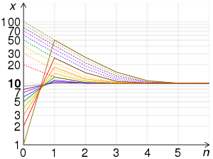
Semilog graphs comparing the speed of convergence of Heron’s method to find the square root of 100 for different initial guesses. Negative guesses converge to the negative root, positive guesses to the positive root. Note that values closer to the root converge faster, and all approximations are overestimates. In the SVG file, hover over a graph to display its points.
Suppose that x0 > 0 and S > 0. Then for any natural number n, xn > 0. Let the relative error in xn be defined by

and thus

Then it can be shown that

And thus that

and consequently that convergence is assured, and quadratic.
Worst case for convergence[edit]
If using the rough estimate above with the Babylonian method, then the least accurate cases in ascending order are as follows:

Thus in any case,


Rounding errors will slow the convergence. It is recommended to keep at least one extra digit beyond the desired accuracy of the xn being calculated to minimize round off error.
Bakhshali method[edit]
This method for finding an approximation to a square root was described in an ancient South Asian manuscript from Pakistan, called the Bakhshali manuscript. It is equivalent to two iterations of the Babylonian method beginning with x0. Thus, the algorithm is quartically convergent, which means that the number of correct digits of the approximation roughly quadruples with each iteration.[3] The original presentation, using modern notation, is as follows: To calculate , let  be the initial approximation to . Then, successively iterate as:

This can be used to construct a rational approximation to the square root by beginning with an integer. If  is an integer chosen so
  is close to , and
  is the difference whose absolute value is minimized, then the first iteration can be written as:

The Bakhshali method can be generalized to the computation of an arbitrary root, including fractional roots.[4]
Example[edit]
Using the same example as given with the Babylonian method, let  Then, the first iteration gives

Likewise the second iteration gives

Digit-by-digit calculation[edit]
This is a method to find each digit of the square root in a sequence. This method is based on the binomial theorem and basically an inverse algorithm solving  . It is slower than the Babylonian method, but it has several advantages:
- It can be easier for manual calculations.
- Every digit of the root found is known to be correct, i.e., it does not have to be changed later.
- If the square root has an expansion that terminates, the algorithm terminates after the last digit is found. Thus, it can be used to check whether a given integer is a square number.
- The algorithm works for any base, and naturally, the way it proceeds depends on the base chosen.
- Inconveniences are that the algorithm becomes quite unhandleable for higher roots and that it is not allowing inaccurate guesses or inaccurate sub-calculations as they, unlike the self correcting approximations like with Newton’s method, lead to every following digit of the result being wrong. Furthermore this algorithm, even though being efficient enough on paper, is way too expensive for software implementations as the many calculations become larger and larger and load the memory while still only allowing digit by digit progressions leading the algorithm to become slower and slower with every following digit.
Napier’s bones include an aid for the execution of this algorithm. The shifting nth root algorithm is a generalization of this method.
Basic principle[edit]
First, consider the case of finding the square root of a number Z, that is the square of a two-digit number XY, where X is the tens digit and Y is the units digit. Specifically:

Now using the digit-by-digit algorithm, we first determine the value of X. X is the largest digit such that X2 is less than or equal to Z from which we removed the two rightmost digits.
In the next iteration, we pair the digits, multiply X by 2, and place it in the tenth’s place while we try to figure out what the value of Y is.
Since this is a simple case where the answer is a perfect square root XY, the algorithm stops here.
The same idea can be extended to any arbitrary square root computation next. Suppose we are able to find the square root of N by expressing it as a sum of n positive numbers such that
- .

By repeatedly applying the basic identity

the right-hand-side term can be expanded as
![{begin{aligned}&(a_{1}+a_{2}+a_{3}+dotsb +a_{n})^{2}\=&,a_{1}^{2}+2a_{1}a_{2}+a_{2}^{2}+2(a_{1}+a_{2})a_{3}+a_{3}^{2}+dotsb +a_{n-1}^{2}+2left(sum _{i=1}^{n-1}a_{i}right)a_{n}+a_{n}^{2}\=&,a_{1}^{2}+[2a_{1}+a_{2}]a_{2}+[2(a_{1}+a_{2})+a_{3}]a_{3}+dotsb +left[2left(sum _{i=1}^{n-1}a_{i}right)+a_{n}right]a_{n}.end{aligned}}](https://wikimedia.org/api/rest_v1/media/math/render/svg/3c9fc9912ec91d9fa1e6a5ca9c5d1c5b98ec6316)
This expression allows us to find the square root by sequentially guessing the values of  s. Suppose that the numbers
  have already been guessed, then the m-th term of the right-hand-side of above summation is given by
 ![Y_{m}=[2P_{m-1}+a_{m}]a_{m},](https://wikimedia.org/api/rest_v1/media/math/render/svg/5f44cbdda22b202c32f5420b0ab8051e609ffe16) where
where  is the approximate square root found so far. Now each new guess
  should satisfy the recursion

such that  for all
  with initialization
  When
When  the exact square root has been found; if not, then the sum of s gives a suitable approximation of the square root, with
  being the approximation error.
For example, in the decimal number system we have

where  are place holders and the coefficients
  . At any m-th stage of the square root calculation, the approximate root found so far,
  and the summation term
  are given by

![{displaystyle Y_{m}=[2P_{m-1}+a_{m}cdot 10^{n-m}]a_{m}cdot 10^{n-m}=left[20sum _{i=1}^{m-1}a_{i}cdot 10^{m-i-1}+a_{m}right]a_{m}cdot 10^{2(n-m)}.}](https://wikimedia.org/api/rest_v1/media/math/render/svg/665e9765734e1824ef3b9675155242ac283fef2f)
Here since the place value of is an even power of 10, we only need to work with the pair of most significant digits of the remaining term  at any m-th stage. The section below codifies this procedure.
It is obvious that a similar method can be used to compute the square root in number systems other than the decimal number system. For instance, finding the digit-by-digit square root in the binary number system is quite efficient since the value of is searched from a smaller set of binary digits {0,1}. This makes the computation faster since at each stage the value of is either  for
for  or
or  for
for  . The fact that we have only two possible options for also makes the process of deciding the value of at m-th stage of calculation easier. This is because we only need to check if
  for
for  If this condition is satisfied, then we take ; if not then
  Also, the fact that multiplication by 2 is done by left bit-shifts helps in the computation.
Decimal (base 10)[edit]
Write the original number in decimal form. The numbers are written similar to the long division algorithm, and, as in long division, the root will be written on the line above. Now separate the digits into pairs, starting from the decimal point and going both left and right. The decimal point of the root will be above the decimal point of the square. One digit of the root will appear above each pair of digits of the square.
Beginning with the left-most pair of digits, do the following procedure for each pair:
- Starting on the left, bring down the most significant (leftmost) pair of digits not yet used (if all the digits have been used, write «00») and write them to the right of the remainder from the previous step (on the first step, there will be no remainder). In other words, multiply the remainder by 100 and add the two digits. This will be the current value c.
- Find p, y and x, as follows:
- Subtract y from c to form a new remainder.
- If the remainder is zero and there are no more digits to bring down, then the algorithm has terminated. Otherwise go back to step 1 for another iteration.
Examples[edit]
Find the square root of 152.2756.
          1  2. 3  4
       /
     /  01 52.27 56

         01                   1*1 <= 1 < 2*2                 x = 1
         01                     y = x*x = 1*1 = 1
         00 52                22*2 <= 52 < 23*3              x = 2
         00 44                  y = (20+x)*x = 22*2 = 44
            08 27             243*3 <= 827 < 244*4           x = 3
            07 29               y = (240+x)*x = 243*3 = 729
               98 56          2464*4 <= 9856 < 2465*5        x = 4
               98 56            y = (2460+x)*x = 2464*4 = 9856
               00 00          Algorithm terminates: Answer is 12.34
Binary numeral system (base 2)[edit]
This section uses the formalism from the digit-by-digit calculation section above, with the slight variation that we let  , with each
  or .
or .
We iterate all  , from
  down to
  , and build up an approximate solution
  , the sum of all for which we have determined the value.
To determine if equals or  , we let
  . If
. If  (i.e. the square of our approximate solution including does not exceed the target square) then , otherwise and
  .
.
To avoid squaring  in each step, we store the difference
  and incrementally update it by setting
  with
with  .
.
Initially, we set  for the largest
  with
with  .
.
As an extra optimization, we store  and
and  , the two terms of in case that is nonzero, in separate variables
  ,
,  :
:


and can be efficiently updated in each step:


Note that:
- , which is the final result returned in the function below.

An implementation of this algorithm in C:[5]
int32_t isqrt(int32_t n) {
    assert(("sqrt input should be non-negative", n > 0));

    // Xₙ₊₁
    int32_t x = n;

    // cₙ
    int32_t c = 0;

    // dₙ which starts at the highest power of four <= n
    int32_t d = 1 << 30; // The second-to-top bit is set.
                         // Same as ((unsigned) INT32_MAX + 1) / 2.
    while (d > n)
        d >>= 2;

    // for dₙ … d₀
    while (d != 0) {
        if (x >= c + d) {      // if Xₘ₊₁ ≥ Yₘ then aₘ = 2ᵐ
            x -= c + d;        // Xₘ = Xₘ₊₁ - Yₘ
            c = (c >> 1) + d;  // cₘ₋₁ = cₘ/2 + dₘ (aₘ is 2ᵐ)
        }
        else {
            c >>= 1;           // cₘ₋₁ = cₘ/2      (aₘ is 0)
        }
        d >>= 2;               // dₘ₋₁ = dₘ/4
    }
    return c;                  // c₋₁
}
Faster algorithms, in binary and decimal or any other base, can be realized by using lookup tables—in effect trading more storage space for reduced run time.[6]
Exponential identity[edit]
Pocket calculators typically implement good routines to compute the exponential function and the natural logarithm, and then compute the square root of S using the identity found using the properties of logarithms ( ) and exponentials (
 ):[citation needed]

The denominator in the fraction corresponds to the nth root. In the case above the denominator is 2, hence the equation specifies that the square root is to be found. The same identity is used when computing square roots with logarithm tables or slide rules.
A two-variable iterative method[edit]
This method is applicable for finding the square root of  and converges best for
  .
.
This, however, is no real limitation for a computer based calculation, as in base 2 floating point and fixed point representations, it is trivial to multiply  by an integer power of 4, and therefore by the corresponding power of 2, by changing the exponent or by shifting, respectively. Therefore, can be moved to the range
  . Moreover, the following method does not employ general divisions, but only additions, subtractions, multiplications, and divisions by powers of two, which are again trivial to implement. A disadvantage of the method is that numerical errors accumulate, in contrast to single variable iterative methods such as the Babylonian one.
The initialization step of this method is


while the iterative steps read


Then,  (while
  ).
).
The convergence of  , and therefore also of
  , is quadratic.
The proof of the method is rather easy. First, rewrite the iterative definition of as
- .

Then it is straightforward to prove by induction that

and therefore the convergence of to the desired result is ensured by the convergence of to 0, which in turn follows from  .
.
This method was developed around 1950 by M. V. Wilkes, D. J. Wheeler and S. Gill[7] for use on EDSAC, one of the first electronic computers.[8] The method was later generalized, allowing the computation of non-square roots.[9]
Iterative methods for reciprocal square roots[edit]
The following are iterative methods for finding the reciprocal square root of S which is  . Once it has been found, find by simple multiplication:
  . These iterations involve only multiplication, and not division. They are therefore faster than the Babylonian method. However, they are not stable. If the initial value is not close to the reciprocal square root, the iterations will diverge away from it rather than converge to it. It can therefore be advantageous to perform an iteration of the Babylonian method on a rough estimate before starting to apply these methods.
Goldschmidt’s algorithm[edit]
Some computers use Goldschmidt’s algorithm to simultaneously calculate
and
.
Goldschmidt’s algorithm finds faster than Newton-Raphson iteration on a computer with a fused multiply–add instruction and either a pipelined floating point unit or two independent floating-point units.[10]
The first way of writing Goldschmidt’s algorithm begins
- (typically using a table lookup)


and iterates


until  is sufficiently close to 1, or a fixed number of iterations. The iterations converge to
- , and
- .


Note that it is possible to omit either  and
and  from the computation, and if both are desired then
  may be used at the end rather than computing it through in each iteration.
A second form, using fused multiply-add operations, begins
- (typically using a table lookup)


and iterates


until  is sufficiently close to 0, or a fixed number of iterations. This converges to
- , and
- .

Taylor series[edit]
If N is an approximation to , a better approximation can be found by using the Taylor series of the square root function:

As an iterative method, the order of convergence is equal to the number of terms used. With two terms, it is identical to the Babylonian method. With three terms, each iteration takes almost as many operations as the Bakhshali approximation, but converges more slowly.[citation needed] Therefore, this is not a particularly efficient way of calculation. To maximize the rate of convergence, choose N so that  is as small as possible.
Continued fraction expansion[edit]
Quadratic irrationals (numbers of the form  , where a, b and c are integers), and in particular, square roots of integers, have periodic continued fractions. Sometimes what is desired is finding not the numerical value of a square root, but rather its continued fraction expansion, and hence its rational approximation. Let S be the positive number for which we are required to find the square root. Then assuming a to be a number that serves as an initial guess and r to be the remainder term, we can write
  Since we have
  , we can express the square root of S as

By applying this expression for to the denominator term of the fraction, we have

Compact notation
The numerator/denominator expansion for continued fractions (see left) is cumbersome to write as well as to embed in text formatting systems. So mathematicians have devised several alternative notations, like[11]

When  throughout, an even more compact notation is:[12]
![{displaystyle [a;2a,2a,2a,cdots ]}](https://wikimedia.org/api/rest_v1/media/math/render/svg/e99050ef07e1bf563b7ce6836c08328e4a9e3051)
For repeating continued fractions (which all square roots of non-perfect squares do), the repetend is represented only once, with an overline to signify a non-terminating repetition of the overlined part:[13]
![{displaystyle [a;{overline {2a}}]}](https://wikimedia.org/api/rest_v1/media/math/render/svg/b5b579e3cc5ede7bcb2db3f3b18b80dd1d2e9d3a)
For √2, the value of is 1, so its representation is:
Proceeding this way, we get a generalized continued fraction for the square root as

The first step to evaluating such a fraction[14] to obtain a root is to do numerical substitutions for the root of the number desired, and number of denominators selected. For example, in canonical form,  is 1 and for √2, is 1, so the numerical continued fraction for 3 denominators is:

Step 2 is to reduce the continued fraction from the bottom up, one denominator at a time, to yield a rational fraction whose numerator and denominator are integers. The reduction proceeds thus (taking the first three denominators):


Finally (step 3), divide the numerator by the denominator of the rational fraction to obtain the approximate value of the root:
- rounded to three digits of precision.

The actual value of √2 is 1.41 to three significant digits. The relative error is 0.17%, so the rational fraction is good to almost three digits of precision. Taking more denominators gives successively better approximations: four denominators yields the fraction  , good to almost 4 digits of precision, etc.
The following are examples of square roots, their simple continued fractions, and their first terms — called convergents — up to and including denominator 99:
| √S | ~decimal | continued fraction | convergents |
|---|---|---|---|
| √2 | 1.41421 | ![{displaystyle [1;{overline {2}}]}](https://wikimedia.org/api/rest_v1/media/math/render/svg/076639b7e958148e44b2dfe0bea22fca5b382c6f)
|

|
| √3 | 1.73205 | ![{displaystyle [1;{overline {1,2}}]}](https://wikimedia.org/api/rest_v1/media/math/render/svg/118ba741c0676d2c89508d125b151ab4d17b94eb)
|

|
| √5 | 2.23607 | ![{displaystyle [2;{overline {4}}]}](https://wikimedia.org/api/rest_v1/media/math/render/svg/574efb17309ec89c6733471fb7482deef730fafc)
|

|
| √6 | 2.44949 | ![{displaystyle [2;{overline {2,4}}]}](https://wikimedia.org/api/rest_v1/media/math/render/svg/d5f8f79da35588663e839e36b8447e741b651576)
|

|
| √10 | 3.16228 | ![{displaystyle [3;{overline {6}}]}](https://wikimedia.org/api/rest_v1/media/math/render/svg/d7e53c2d8b2dff31b1a66bf6179455be532d3a93)
|

|

|
1.77245 | ![{displaystyle [1;1,3,2,1,1,6...]}](https://wikimedia.org/api/rest_v1/media/math/render/svg/7dc1ddad6bd13b951e89a900cadeaab3a1770c74)
|

|

|
1.64872 | ![{displaystyle [1;1,1,1,5,1,1...]}](https://wikimedia.org/api/rest_v1/media/math/render/svg/4dc729725d22fec6931be55fdeb24281625abc18)
|

|

|
1.27202 | ![{displaystyle [1;3,1,2,11,3,7...]}](https://wikimedia.org/api/rest_v1/media/math/render/svg/4c2b676231a4a5d8ae24101d610ec5465334869a)
|

|
In general, the larger the denominator of a rational fraction, the better the approximation. It can also be shown that truncating a continued fraction yields a rational fraction that is the best approximation to the root of any fraction with denominator less than or equal to the denominator of that fraction — e.g., no fraction with a denominator less than or equal to 70 is as good an approximation to √2 as 99/70.
Lucas sequence method[edit]
the Lucas sequence of the first kind Un(P,Q) is defined by the recurrence relations:

and the characteristic equation of it is:

it has the discriminant  and the roots:

all that yield the following positive value:

so when we want , we can choose  and
and  , and then calculate
  using
using  and
and  for large value of .
The most effective way to calculate and is:

Summary:

then when  :
:

Approximations that depend on the floating point representation[edit]
A number is represented in a floating point format as  which is also called scientific notation. Its square root is
  and similar formulae would apply for cube roots and logarithms. On the face of it, this is no improvement in simplicity, but suppose that only an approximation is required: then just
  is good to an order of magnitude. Next, recognise that some powers, p, will be odd, thus for 3141.59 = 3.14159×10³ rather than deal with fractional powers of the base, multiply the mantissa by the base and subtract one from the power to make it even. The adjusted representation will become the equivalent of 31.4159×10² so that the square root will be √31.4159×101.
If the integer part of the adjusted mantissa is taken, there can only be the values 1 to 99, and that could be used as an index into a table of 99 pre-computed square roots to complete the estimate. A computer using base sixteen would require a larger table, but one using base two would require only three entries: the possible bits of the integer part of the adjusted mantissa are 01 (the power being even so there was no shift, remembering that a normalised floating point number always has a non-zero high-order digit) or if the power was odd, 10 or 11, these being the first two bits of the original mantissa. Thus, 6.25 = 110.01 in binary, normalised to 1.1001 × 22 an even power so the paired bits of the mantissa are 01, while .625 = 0.101 in binary normalises to 1.01 × 2−1 an odd power so the adjustment is to 10.1 × 2−2 and the paired bits are 10. Notice that the low order bit of the power is echoed in the high order bit of the pairwise mantissa. An even power has its low-order bit zero and the adjusted mantissa will start with 0, whereas for an odd power that bit is one and the adjusted mantissa will start with 1. Thus, when the power is halved, it is as if its low order bit is shifted out to become the first bit of the pairwise mantissa.
A table with only three entries could be enlarged by incorporating additional bits of the mantissa. However, with computers, rather than calculate an interpolation into a table, it is often better to find some simpler calculation giving equivalent results. Everything now depends on the exact details of the format of the representation, plus what operations are available to access and manipulate the parts of the number. For example, Fortran offers an EXPONENT(x) function to obtain the power. Effort expended in devising a good initial approximation is to be recouped by thereby avoiding the additional iterations of the refinement process that would have been needed for a poor approximation. Since these are few (one iteration requires a divide, an add, and a halving) the constraint is severe.
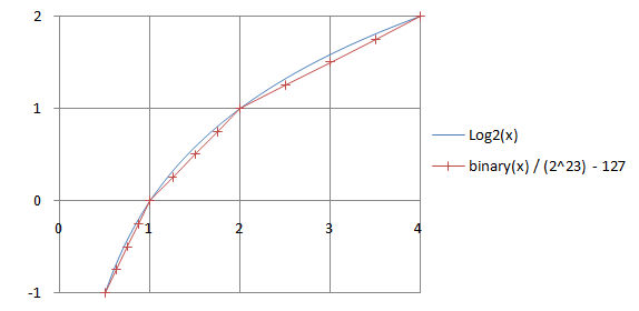
Many computers follow the IEEE (or sufficiently similar) representation, and a very rapid approximation to the square root can be obtained for starting Newton’s method. The technique that follows is based on the fact that the floating point format (in base two) approximates the base-2 logarithm. That is 
So for a 32-bit single precision floating point number in IEEE format (where notably, the power has a bias of 127 added for the represented form) you can get the approximate logarithm by interpreting its binary representation as a 32-bit integer, scaling it by  , and removing a bias of 127, i.e.

For example, 1.0 is represented by a hexadecimal number 0x3F800000, which would represent  if taken as an integer. Using the formula above you get
  , as expected from
  . In a similar fashion you get 0.5 from 1.5 (0x3FC00000).
To get the square root, divide the logarithm by 2 and convert the value back. The following program demonstrates the idea. The exponent’s lowest bit is intentionally allowed to propagate into the mantissa. One way to justify the steps in this program is to assume  is the exponent bias and is the number of explicitly stored bits in the mantissa and then show that

/* Assumes that float is in the IEEE 754 single precision floating point format */
#include <stdint.h>
float sqrt_approx(float z)
{
	union { float f; uint32_t i; } val = {z};	/* Convert type, preserving bit pattern */
	/*
	 * To justify the following code, prove that
	 *
	 * ((((val.i / 2^m) - b) / 2) + b) * 2^m = ((val.i - 2^m) / 2) + ((b + 1) / 2) * 2^m)
	 *
	 * where
	 *
	 * b = exponent bias
	 * m = number of mantissa bits
	 */
	val.i -= 1 << 23;	/* Subtract 2^m. */
	val.i >>= 1;		/* Divide by 2. */
	val.i += 1 << 29;	/* Add ((b + 1) / 2) * 2^m. */

	return val.f;		/* Interpret again as float */
}
The three mathematical operations forming the core of the above function can be expressed in a single line. An additional adjustment can be added to reduce the maximum relative error. So, the three operations, not including the cast, can be rewritten as
val.i = (1 << 29) + (val.i >> 1) - (1 << 22) + a;
where a is a bias for adjusting the approximation errors. For example, with a = 0 the results are accurate for even powers of 2 (e.g. 1.0), but for other numbers the results will be slightly too big (e.g. 1.5 for 2.0 instead of 1.414… with 6% error). With a = −0x4B0D2, the maximum relative error is minimized to ±3.5%.
If the approximation is to be used for an initial guess for Newton’s method to the equation  , then the reciprocal form shown in the following section is preferred.
Reciprocal of the square root[edit]
A variant of the above routine is included below, which can be used to compute the reciprocal of the square root, i.e.,  instead, was written by Greg Walsh. The integer-shift approximation produced a relative error of less than 4%, and the error dropped further to 0.15% with one iteration of Newton’s method on the following line.[15] In computer graphics it is a very efficient way to normalize a vector.
float invSqrt(float x) {
    float xhalf = 0.5f * x;
    union {
        float x;
        int i;
    } u;
    u.x = x;
    u.i = 0x5f375a86 - (u.i >> 1);
    /* The next line can be repeated any number of times to increase accuracy */
    u.x = u.x * (1.5f - xhalf * u.x * u.x);
    return u.x;
}
Some VLSI hardware implements inverse square root using a second degree polynomial estimation followed by a Goldschmidt iteration.[16]
Negative or complex square[edit]
If S < 0, then its principal square root is

If S = a+bi where a and b are real and b ≠ 0, then its principal square root is

This can be verified by squaring the root.[17][18]
Here

is the modulus of S. The principal square root of a complex number is defined to be the root with the non-negative real part.
See also[edit]
- Alpha max plus beta min algorithm
- nth root algorithm
- Square root of 2
- Integer square root
Notes[edit]
References[edit]
- ^ Fowler & Robson 1998.
- ^ Heath 1921.
- ^ Bailey & Borwein 2012.
- ^ Simply Curious 2018.
- ^ Guy & UKC 1985.
- ^ Steinarson, Corbit & Hendry 2003.
- ^ Wilkes, Wheeler & Gill 1951.
- ^ Campbell-Kelly 2009.
- ^ Gower 1958.
- ^ Markstein 2004.
- ^ see: Generalized continued fraction#Notation
- ^ see: Continued fraction#Notations
- ^ see: Periodic continued fraction
- ^ Sardina 2007, 2.3j on p.10.
- ^ Lomont 2003.
- ^ Piñeiro & Díaz Bruguera 2002.
- ^ Abramowitz & Stegun 1964, Section 3.7.26.
- ^ Cooke 2008.
Bibliography[edit]
Abramowitz, Miltonn; Stegun, Irene A. (1964). Handbook of mathematical functions with formulas, graphs, and mathematical tables. Courier Dover Publications. p. 17. ISBN 978-0-486-61272-0.
Bailey, David; Borwein, Jonathan (2012). «Ancient Indian Square Roots: An Exercise in Forensic Paleo-Mathematics» (PDF). American Mathematical Monthly. Vol. 119, no. 8. pp. 646–657. Retrieved 2017-09-14.
Campbell-Kelly, Martin (September 2009). «Origin of Computing». Scientific American. 301 (3): 62–69. Bibcode:2009SciAm.301c..62C. doi:10.1038/scientificamerican0909-62. JSTOR 26001527. PMID 19708529.
Cooke, Roger (2008). Classical algebra: its nature, origins, and uses. John Wiley and Sons. p. 59. ISBN 978-0-470-25952-8.
Fowler, David; Robson, Eleanor (1998). «Square Root Approximations in Old Babylonian Mathematics: YBC 7289 in Context» (PDF). Historia Mathematica. 25 (4): 376. doi:10.1006/hmat.1998.2209.
Gower, John C. (1958). «A Note on an Iterative Method for Root Extraction». The Computer Journal. 1 (3): 142–143. doi:10.1093/comjnl/1.3.142.
Guy, Martin; UKC (1985). «Fast integer square root by Mr. Woo’s abacus algorithm (archived)». Archived from the original on 2012-03-06.
Heath, Thomas (1921). A History of Greek Mathematics, Vol. 2. Oxford: Clarendon Press. pp. 323–324.
Lomont, Chris (2003). «Fast Inverse Square Root» (PDF).
Markstein, Peter (November 2004). Software Division and Square Root Using Goldschmidt’s Algorithms (PDF). 6th Conference on Real Numbers and Computers. Dagstuhl, Germany. CiteSeerX 10.1.1.85.9648.
Piñeiro, José-Alejandro; Díaz Bruguera, Javier (December 2002). «High-Speed Double-Precision Computationof Reciprocal, Division, Square Root, and Inverse Square Root». IEEE Transactions on Computers. 51 (12): 1377–1388. doi:10.1109/TC.2002.1146704.
Sardina, Manny (2007). «General Method for Extracting Roots using (Folded) Continued Fractions». Surrey (UK).
Simply Curious (5 June 2018). «Bucking down to the Bakhshali manuscript». Simply Curious blog. Retrieved 2020-12-21.
Steinarson, Arne; Corbit, Dann; Hendry, Mathew (2003). «Integer Square Root function».
Wilkes, M.V.; Wheeler, D.J.; Gill, S. (1951). The Preparation of Programs for an Electronic Digital Computer. Oxford: Addison-Wesley. pp. 323–324. OCLC 475783493.
External links[edit]
- Weisstein, Eric W. «Square root algorithms». MathWorld.
- Square roots by subtraction
- Integer Square Root Algorithm by Andrija Radović
- Personal Calculator Algorithms I : Square Roots (William E. Egbert), Hewlett-Packard Journal (May 1977) : page 22
- Calculator to learn the square root
Время на прочтение
1 мин
Количество просмотров 29K
Серия постов [Неочевидные алгоритмы очевидных вещей] будет содержать алгоритмы действий, которые кажутся очевидными и простыми, но если задать себе вопрос «как это делается?», то ответ является далеко не очевидным. Разумеется, все эти алгоритмы можно найти в литературе. Под катом располагается алгоритм вычисления корня квадратного числа X.
Корень квадаратный числа Х
Идея
Формируется прямоугольник со сторонами a=1 и b=X. Площадь этого прямоугольника равна S = a * b = X * 1 = X. Преобразовав прямоугольник в квадрат так, что его площадь останется прежней, получим длину стороны, равную корню квадратному из площади фигуры, которая равна Х.
Каждая итерация преобразования прямоугольника в квадрат производится следующим образом:
S = a0 b0;
Создаётся новый четырёхугольник, который имеет одну сторону, равную среднему арифметическому сторон текущего прямоугольника, но площадь такую же:
S = a1 b1, где a1 = (a0+b0) / 2, а b1=S / a1
S = a2 b2, где a2 = (a1+b1) / 2, а b2=S / a2
…
S = an bn, где an = (an-1+bn-1) / 2, а bn=S / an
И так до тех пор пока не |an-bn| < Eps.
Код функции
#define EPS 1e-10
float my_sqrt(float x){
  float S=x, a=1,b=x;
  while(fabs(a-b)>EPS){  a=(a+b)/2; b = S / a;}
  return (a+b)/2;
}
Как быстро извлекать квадратные корни
14 декабря 2012
Довольно часто при решении задач мы сталкиваемся с большими числами, из которых надо извлечь квадратный корень. Многие ученики решают, что это ошибка, и начинают перерешивать весь пример. Ни в коем случае нельзя так поступать! На то есть две причины:
- Корни из больших чисел действительно встречаются в задачах. Особенно в текстовых;
- Существует алгоритм, с помощью которого эти корни считаются почти устно.
Этот алгоритм мы сегодня и рассмотрим. Возможно, какие-то вещи покажутся вам непонятными. Но если вы внимательно отнесетесь к этому уроку, то получите мощнейшее оружие против квадратных корней.
Итак, алгоритм:
- Ограничить искомый корень сверху и снизу числами, кратными 10. Таким образом, мы сократим диапазон поиска до 10 чисел;
- Из этих 10 чисел отсеять те, которые точно не могут быть корнями. В результате останутся 1—2 числа;
- Возвести эти 1—2 числа в квадрат. То из них, квадрат которого равен исходному числу, и будет корнем.
Прежде чем применять этот алгоритм работает на практике, давайте посмотрим на каждый отдельный шаг.
Ограничение корней
В первую очередь надо выяснить, между какими числами расположен наш корень. Очень желательно, чтобы числа были кратны десяти:
102 = 100;
202 = 400;
302 = 900;
402 = 1600;
…
902 = 8100;
1002 = 10 000.
Получим ряд чисел:
100; 400; 900; 1600; 2500; 3600; 4900; 6400; 8100; 10 000.
Что нам дают эти числа? Все просто: мы получаем границы. Возьмем, например, число 1296. Оно лежит между 900 и 1600. Следовательно, его корень не может быть меньше 30 и больше 40:
![]()
То же самое — с любым другим числом, из которого можно найти квадратный корень. Например, 3364:
![]()
Таким образом, вместо непонятного числа мы получаем вполне конкретный диапазон, в котором лежит исходный корень. Чтобы еще больше сузить область поиска, переходим ко второму шагу.
Отсев заведомо лишних чисел
Итак, у нас есть 10 чисел — кандидатов на корень. Мы получили их очень быстро, без сложных размышлений и умножений в столбик. Пора двигаться дальше.
Не поверите, но сейчас мы сократим количество чисел-кандидатов до двух — и снова без каких-либо сложных вычислений! Достаточно знать специальное правило. Вот оно:
Последняя цифра квадрата зависит только от последней цифры исходного числа.
Другими словами, достаточно взглянуть на последнюю цифру квадрата — и мы сразу поймем, на что заканчивается исходное число.
Существует всего 10 цифр, которые могут стоять на последнем месте. Попробуем выяснить, во что они превращаются при возведении в квадрат. Взгляните на таблицу:
| 1 | 2 | 3 | 4 | 5 | 6 | 7 | 8 | 9 | 0 |
| 1 | 4 | 9 | 6 | 5 | 6 | 9 | 4 | 1 | 0 |
Эта таблица — еще один шаг на пути к вычислению корня. Как видите, цифры во второй строке оказались симметричными относительно пятерки. Например:
22 = 4;
82 = 64 → 4.
Как видите, последняя цифра в обоих случаях одинакова. А это значит, что, например, корень из 3364 обязательно заканчивается на 2 или на 8. С другой стороны, мы помним ограничение из предыдущего пункта. Получаем:
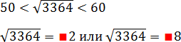
Красные квадраты показывают, что мы пока не знаем этой цифры. Но ведь корень лежит в пределах от 50 до 60, на котором есть только два числа, оканчивающихся на 2 и 8:
![]()
Вот и все! Из всех возможных корней мы оставили всего два варианта! И это в самом тяжелом случае, ведь последняя цифра может быть 5 или 0. И тогда останется единственный кандидат в корни!
Финальные вычисления
Итак, у нас осталось 2 числа-кандидата. Как узнать, какое из них является корнем? Ответ очевиден: возвести оба числа в квадрат. То, которое в квадрате даст исходное число, и будет корнем.
Например, для числа 3364 мы нашли два числа-кандидата: 52 и 58. Возведем их в квадрат:
522 = (50 +2)2 = 2500 + 2 · 50 · 2 + 4 = 2704;
582 = (60 − 2)2 = 3600 − 2 · 60 · 2 + 4 = 3364.
Вот и все! Получилось, что корень равен 58! При этом, чтобы упростить вычисления, я воспользовался формулой квадратов суммы и разности. Благодаря чему даже не пришлось умножать числа в столбик! Это еще один уровень оптимизации вычислений, но, разумеется, совершенно не обязательный 
Примеры вычисления корней
Теория — это, конечно, хорошо. Но давайте проверим ее на практике.
Задача. Вычислите квадратный корень:
[Подпись к рисунку]
Для начала выясним, между какими числами лежит число 576:
400 < 576 < 900
202 < 576 < 302
Теперь смотрим на последнюю цифру. Она равна 6. Когда это происходит? Только если корень заканчивается на 4 или 6. Получаем два числа:
24; 26.
Осталось возвести каждое число в квадрат и сравнить с исходным:
242 = (20 + 4)2 = 576
Отлично! Первый же квадрат оказался равен исходному числу. Значит, это и есть корень.
Задача. Вычислите квадратный корень:
[Подпись к рисунку]
Здесь и далее я буду писать только основные шаги. Итак, ограничиваем число:
900 < 1369 < 1600;
302 < 1369 < 402;
Смотрим на последнюю цифру:
1369 → 9;
33; 37.
Возводим в квадрат:
332 = (30 + 3)2 = 900 + 2 · 30 · 3 + 9 = 1089 ≠ 1369;
372 = (40 − 3)2 = 1600 − 2 · 40 · 3 + 9 = 1369.
Вот и ответ: 37.
Задача. Вычислите квадратный корень:
[Подпись к рисунку]
Ограничиваем число:
2500 < 2704 < 3600;
502 < 2704 < 602;
Смотрим на последнюю цифру:
2704 → 4;
52; 58.
Возводим в квадрат:
522 = (50 + 2)2 = 2500 + 2 · 50 · 2 + 4 = 2704;
Получили ответ: 52. Второе число возводить в квадрат уже не потребуется.
Задача. Вычислите квадратный корень:
[Подпись к рисунку]
Ограничиваем число:
3600 < 4225 < 4900;
602 < 4225 < 702;
Смотрим на последнюю цифру:
4225 → 5;
65.
Как видим, после второго шага остался лишь один вариант: 65. Это и есть искомый корень. Но давайте все-таки возведем его в квадрат и проверим:
652 = (60 + 5)2 = 3600 + 2 · 60 · 5 + 25 = 4225;
Все правильно. Записываем ответ.
Заключение
Многие спрашивают: зачем вообще считать такие корни? Не лучше ли взять калькулятор и не парить себе мозг?
Увы, не лучше. Давайте разберемся в причинах. Их две:
- На любом нормальном экзамене по математике, будь то ГИА или ЕГЭ, пользоваться калькуляторами запрещено. И за пронесенный в класс калькулятор могут запросто выгнать с экзамена.
- Не уподобляйтесь тупым американцам. Которые не то что корни — они два простых числа сложить не могут. А при виде дробей у них вообще начинается истерика.
В общем, учитесь считать. И все будет хорошо. Удачи!
Смотрите также:
- Выделение полного квадрата

- Преобразование выражений с корнем — часть 1

- Знаки тригонометрических функций
- Задача B1 — время, числа и проценты
- Как решать задачу 18: графический подход

- Задача B2 про комиссию в терминале