Как найти корни многочлена в матлабе

Numeric Roots

The roots function calculates
the roots of a single-variable polynomial represented by a vector
of coefficients.

For example, create a vector to represent the polynomial x2−x−6,
then calculate the roots.

p = [1 -1 -6];
r = roots(p)

By convention, MATLAB^® returns the roots in a column vector.

The poly function converts
the roots back to polynomial coefficients. When operating on vectors, poly and roots are
inverse functions, such that poly(roots(p)) returns p (up
to roundoff error, ordering, and scaling).

When operating on a matrix, the poly function
computes the characteristic polynomial of the matrix. The roots of
the characteristic polynomial are the eigenvalues of the matrix. Therefore, roots(poly(A)) and eig(A) return
the same answer (up to roundoff error, ordering, and scaling).

Roots Using Substitution

You can solve polynomial equations involving trigonometric functions by simplifying the equation using a substitution. The resulting polynomial of one variable no longer contains any trigonometric functions.

For example, find the values of θ that solve the equation

3cos2(θ)-sin(θ)+3=0.

Use the fact that cos2(θ)=1-sin2(θ) to express the equation entirely in terms of sine functions:

-3sin2(θ)-sin(θ)+6=0.

Use the substitution x=sin(θ) to express the equation as a simple polynomial equation:

-3×2-x+6=0.

Create a vector to represent the polynomial.

Find the roots of the polynomial.

To undo the substitution, use θ=sin-1(x). The asin function calculates the inverse sine.

theta = 2×1 complex

  -1.5708 + 1.0395i
   1.5708 - 0.7028i

Verify that the elements in theta are the values of θ that solve the original equation (within roundoff error).

f = @(Z) 3*cos(Z).^2 - sin(Z) + 3;
f(theta)

ans = 2×1 complex
10-14 ×

  -0.0888 + 0.0647i
   0.2665 + 0.0399i

Roots in a Specific Interval

Use the fzero function to find the roots of a polynomial in a specific interval. Among other uses, this method is suitable if you plot the polynomial and want to know the value of a particular root.

For example, create a function handle to represent the polynomial 3×7+4×6+2×5+4×4+x3+5×2.

p = @(x) 3*x.^7 + 4*x.^6 + 2*x.^5 + 4*x.^4 + x.^3 + 5*x.^2;

Plot the function over the interval [-2,1].

x = -2:0.1:1;
plot(x,p(x))
ylim([-100 50])
grid on
hold on

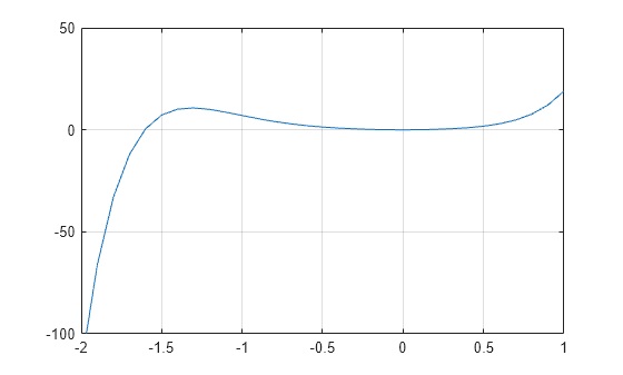
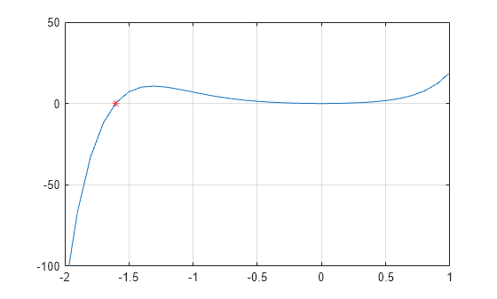
From the plot, the polynomial has a trivial root at 0 and another near -1.5. Use fzero to calculate and plot the root that is near -1.5.

Symbolic Roots

If you have Symbolic Math Toolbox™, then there are additional
options for evaluating polynomials symbolically. One way is to use
the solve (Symbolic Math Toolbox) function.

syms x
s = solve(x^2-x-6)

Another way is to use the factor (Symbolic Math Toolbox) function
to factor the polynomial terms.

See Solve Algebraic Equations (Symbolic Math Toolbox) for more information.