Как найти критическое число рейнольдса - Исправление недочетов и поиск решений вместе с Examum.ru

The plume from this candle flame goes from laminar to turbulent. The Reynolds number can be used to predict where this transition will take place.

The transition from laminar (left) to turbulent (right) flow of water from a tap occurs as the Reynolds number increases.

A vortex street around a cylinder. This can occur around cylinders and spheres, for any fluid, cylinder size, and fluid speed provided that it has a Reynolds number between roughly 40 and 1000.^[1]

In fluid mechanics, the Reynolds number (Re) is a dimensionless quantity that helps predict fluid flow patterns in different situations by measuring the ratio between inertial and viscous forces. At low Reynolds numbers, flows tend to be dominated by laminar (sheet-like) flow, while at high Reynolds numbers, flows tend to be turbulent. The turbulence results from differences in the fluid’s speed and direction, which may sometimes intersect or even move counter to the overall direction of the flow (eddy currents). These eddy currents begin to churn the flow, using up energy in the process, which for liquids increases the chances of cavitation.

The Reynolds number has wide applications, ranging from liquid flow in a pipe to the passage of air over an aircraft wing. It is used to predict the transition from laminar to turbulent flow and is used in the scaling of similar but different-sized flow situations, such as between an aircraft model in a wind tunnel and the full-size version. The predictions of the onset of turbulence and the ability to calculate scaling effects can be used to help predict fluid behavior on a larger scale, such as in local or global air or water movement, and thereby the associated meteorological and climatological effects.

The concept was introduced by George Stokes in 1851,^[2] but the Reynolds number was named by Arnold Sommerfeld in 1908^[3] after Osborne Reynolds (1842–1912), who popularized its use in 1883.^[4]^[5]

Definition[edit]

The Reynolds number is the ratio of inertial forces to viscous forces within a fluid that is subjected to relative internal movement due to different fluid velocities. A region where these forces change behavior is known as a boundary layer, such as the bounding surface in the interior of a pipe. A similar effect is created by the introduction of a stream of high-velocity fluid into a low-velocity fluid, such as the hot gases emitted from a flame in air. This relative movement generates fluid friction, which is a factor in developing turbulent flow. Counteracting this effect is the viscosity of the fluid, which tends to inhibit turbulence. The Reynolds number quantifies the relative importance of these two types of forces for given flow conditions, and is a guide to when turbulent flow will occur in a particular situation.^[6]

This ability to predict the onset of turbulent flow is an important design tool for equipment such as piping systems or aircraft wings, but the Reynolds number is also used in scaling of fluid dynamics problems and is used to determine dynamic similitude between two different cases of fluid flow, such as between a model aircraft, and its full-size version. Such scaling is not linear and the application of Reynolds numbers to both situations allows scaling factors to be developed.

With respect to laminar and turbulent flow regimes:

laminar flow occurs at low Reynolds numbers, where viscous forces are dominant, and is characterized by smooth, constant fluid motion;
turbulent flow occurs at high Reynolds numbers and is dominated by inertial forces, which tend to produce chaotic eddies, vortices and other flow instabilities.^[7]

The Reynolds number is defined as^[3]

${displaystyle mathrm {Re} ={frac {uL}{nu }}={frac {rho uL}{mu }}}$

where:

ρ is the density of the fluid (SI units: kg/m³)
u is the flow speed (m/s)
L is a characteristic linear dimension (m) (see the below sections of this article for examples)
μ is the dynamic viscosity of the fluid (Pa·s or N·s/m² or kg/(m·s))
ν is the kinematic viscosity of the fluid (m²/s).

The Reynolds number can be defined for several different situations where a fluid is in relative motion to a surface.^{[n 1]} These definitions generally include the fluid properties of density and viscosity, plus a velocity and a characteristic length or characteristic dimension (L in the above equation). This dimension is a matter of convention – for example radius and diameter are equally valid to describe spheres or circles, but one is chosen by convention. For aircraft or ships, the length or width can be used. For flow in a pipe, or for a sphere moving in a fluid, the internal diameter is generally used today. Other shapes such as rectangular pipes or non-spherical objects have an equivalent diameter defined. For fluids of variable density such as compressible gases or fluids of variable viscosity such as non-Newtonian fluids, special rules apply. The velocity may also be a matter of convention in some circumstances, notably stirred vessels.

In practice, matching the Reynolds number is not on its own sufficient to guarantee similitude. Fluid flow is generally chaotic, and very small changes to shape and surface roughness of bounding surfaces can result in very different flows. Nevertheless, Reynolds numbers are a very important guide and are widely used.

History[edit]

Osborne Reynolds’s apparatus of 1883 demonstrating the onset of turbulent flow. The apparatus is still at the University of Manchester.

Diagram from Reynolds’s 1883 paper showing onset of turbulent flow.

Osborne Reynolds famously studied the conditions in which the flow of fluid in pipes transitioned from laminar flow to turbulent flow.
In his 1883 paper Reynolds described the transition from laminar to turbulent flow in a classic experiment in which he examined the behaviour of water flow under different flow velocities using a small stream of dyed water introduced into the centre of clear water flow in a larger pipe.

The larger pipe was glass so the behaviour of the layer of the dyed stream could be observed. At the end of this pipe, there was a flow control valve used to vary the water velocity inside the tube. When the velocity was low, the dyed layer remained distinct throughout the entire length of the large tube. When the velocity was increased, the layer broke up at a given point and diffused throughout the fluid’s cross-section. The point at which this happened was the transition point from laminar to turbulent flow.

From these experiments came the dimensionless Reynolds number for dynamic similarity—the ratio of inertial forces to viscous forces. Reynolds also proposed what is now known as the Reynolds averaging of turbulent flows, where quantities such as velocity are expressed as the sum of mean and fluctuating components. Such averaging allows for ‘bulk’ description of turbulent flow, for example using the Reynolds-averaged Navier–Stokes equations.

Flow in a pipe[edit]

For flow in a pipe or tube, the Reynolds number is generally defined as^[8]

${displaystyle mathrm {Re} ={frac {uD_{text{H}}}{nu }}={frac {rho uD_{text{H}}}{mu }}={frac {rho QD_{text{H}}}{mu A}}={frac {WD_{text{H}}}{mu A}},}$

where

D_H is the hydraulic diameter of the pipe (the inside diameter if the pipe is circular) (m),
Q is the volumetric flow rate (m³/s),
A is the pipe’s cross-sectional area (A = πD²/4) (m²),
u is the mean velocity of the fluid (m/s),
μ (mu) is the dynamic viscosity of the fluid (Pa·s = N·s/m² = kg/(m·s)),
ν (nu) is the kinematic viscosity (ν = μ/ρ) (m²/s),
ρ (rho) is the density of the fluid (kg/m³),
W is the mass flowrate of the fluid (kg/s).

For shapes such as squares, rectangular or annular ducts where the height and width are comparable, the characteristic dimension for internal-flow situations is taken to be the hydraulic diameter, D_H, defined as

${displaystyle D_{text{H}}={frac {4A}{P}},}$

where A is the cross-sectional area, and P is the wetted perimeter. The wetted perimeter for a channel is the total perimeter of all channel walls that are in contact with the flow.^[9] This means that the length of the channel exposed to air is not included in the wetted perimeter.

For a circular pipe, the hydraulic diameter is exactly equal to the inside pipe diameter:

${displaystyle D_{text{H}}=D.}$

For an annular duct, such as the outer channel in a tube-in-tube heat exchanger, the hydraulic diameter can be shown algebraically to reduce to

${displaystyle D_{text{H,annulus}}=D_{text{o}}-D_{text{i}},}$

where

D_o is the inside diameter of the outer pipe,
D_i is the outside diameter of the inner pipe.

For calculation involving flow in non-circular ducts, the hydraulic diameter can be substituted for the diameter of a circular duct, with reasonable accuracy, if the aspect ratio AR of the duct cross-section remains in the range 1/4 < AR < 4.^[10]

Laminar–turbulent transition[edit]

In boundary layer flow over a flat plate, experiments confirm that, after a certain length of flow, a laminar boundary layer will become unstable and turbulent. This instability occurs across different scales and with different fluids, usually when Re_x ≈ 5×10⁵,^[11] where x is the distance from the leading edge of the flat plate, and the flow velocity is the freestream velocity of the fluid outside the boundary layer.

For flow in a pipe of diameter D, experimental observations show that for «fully developed» flow,^{[n 2]} laminar flow occurs when Re_D < 2300 and turbulent flow occurs when Re_D > 2900.^[12]^[13] At the lower end of this range, a continuous turbulent-flow will form, but only at a very long distance from the inlet of the pipe. The flow in between will begin to transition from laminar to turbulent and then back to laminar at irregular intervals, called intermittent flow. This is due to the different speeds and conditions of the fluid in different areas of the pipe’s cross-section, depending on other factors such as pipe roughness and flow uniformity. Laminar flow tends to dominate in the fast-moving center of the pipe while slower-moving turbulent flow dominates near the wall. As the Reynolds number increases, the continuous turbulent-flow moves closer to the inlet and the intermittency in between increases, until the flow becomes fully turbulent at Re_D > 2900.^[12] This result is generalized to non-circular channels using the hydraulic diameter, allowing a transition Reynolds number to be calculated for other shapes of channel.^[12]

These transition Reynolds numbers are also called critical Reynolds numbers, and were studied by Osborne Reynolds around 1895.^[5] The critical Reynolds number is different for every geometry.^[14]

Flow in a wide duct[edit]

For a fluid moving between two plane parallel surfaces—where the width is much greater than the space between the plates—then the characteristic dimension is equal to the distance between the plates.^[15] This is consistent with the annular duct and rectangular duct cases above, taken to a limiting aspect ratio.

Flow in an open channel[edit]

For calculating the flow of liquid with a free surface, the hydraulic radius must be determined. This is the cross-sectional area of the channel divided by the wetted perimeter. For a semi-circular channel, it is a quarter of the diameter (in case of full pipe flow). For a rectangular channel, the hydraulic radius is the cross-sectional area divided by the wetted perimeter. Some texts then use a characteristic dimension that is four times the hydraulic radius, chosen because it gives the same value of Re for the onset of turbulence as in pipe flow,^[16] while others use the hydraulic radius as the characteristic length-scale with consequently different values of Re for transition and turbulent flow.

Flow around airfoils[edit]

Reynolds numbers are used in airfoil design to (among other things) manage «scale effect» when computing/comparing characteristics (a tiny wing, scaled to be huge, will perform differently).^[17] Fluid dynamicists define the chord Reynolds number R = Vc/ν, where V is the flight speed, c is the chord length, and ν is the kinematic viscosity of the fluid in which the airfoil operates, which is 1.460×10⁻⁵ m²/s for the atmosphere at sea level.^[18] In some special studies a characteristic length other than chord may be used; rare is the «span Reynolds number», which is not to be confused with span-wise stations on a wing, where chord is still used.^[19]

Object in a fluid[edit]

The high viscosity of honey results in perfectly laminar flow when poured from a bucket, while the low surface tension allows it to remain sheet-like even after reaching the fluid below. Analogous to turbulence, when the flow meets resistance it slows and begins oscillating back and forth, piling upon itself.

The Reynolds number for an object moving in a fluid, called the particle Reynolds number and often denoted Re_p, characterizes the nature of the surrounding flow and its fall velocity.

In viscous fluids[edit]

Creeping flow past a falling sphere: streamlines, drag force F_d and force by gravity F_g.

Where the viscosity is naturally high, such as polymer solutions and polymer melts, flow is normally laminar. The Reynolds number is very small and Stokes’ law can be used to measure the viscosity of the fluid. Spheres are allowed to fall through the fluid and they reach the terminal velocity quickly, from which the viscosity can be determined.

The laminar flow of polymer solutions is exploited by animals such as fish and dolphins, who exude viscous solutions from their skin to aid flow over their bodies while swimming. It has been used in yacht racing by owners who want to gain a speed advantage by pumping a polymer solution such as low molecular weight polyoxyethylene in water, over the wetted surface of the hull.

It is, however, a problem for mixing polymers, because turbulence is needed to distribute fine filler (for example) through the material. Inventions such as the «cavity transfer mixer» have been developed to produce multiple folds into a moving melt so as to improve mixing efficiency. The device can be fitted onto extruders to aid mixing.

Sphere in a fluid[edit]

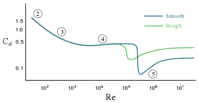
Drag coefficient C_d for a sphere as a function of Reynolds number Re, as obtained from laboratory experiments. The dark line is for a sphere with a smooth surface, while the lighter line is for the case of a rough surface (e.g. with small dimples). There is a range of fluid velocities where a rough-surfaced golf ball experiences less drag than a smooth ball. The numbers along the line indicate several flow regimes and associated changes in the drag coefficient:

attached flow (Stokes flow) and steady separated flow,
separated unsteady flow, having a laminar flow boundary layer upstream of the separation, and producing a vortex street,
separated unsteady flow with a laminar boundary layer at the upstream side, before flow separation, with downstream of the sphere a chaotic turbulent wake,
post-critical separated flow, with a turbulent boundary layer.

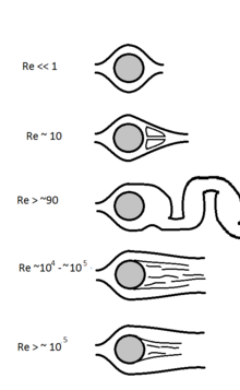
For a sphere in a fluid, the characteristic length-scale is the diameter of the sphere and the characteristic velocity is that of the sphere relative to the fluid some distance away from the sphere, such that the motion of the sphere does not disturb that reference parcel of fluid. The density and viscosity are those belonging to the fluid.^[20] Note that purely laminar flow only exists up to Re = 10 under this definition.

Under the condition of low Re, the relationship between force and speed of motion is given by Stokes’ law.^[21]

At higher Reynolds numbers the drag on a sphere depends on surface roughness. Thus, for example, adding dimples on the surface of a golf ball causes the boundary layer on the upstream side of the ball to transition from laminar to turbulent. The turbulent boundary layer is able to remain attached to the surface of the ball much longer than a laminar boundary and so creates a narrower low-pressure wake and hence less pressure drag. The reduction in pressure drag causes the ball to travel further.^[22]

Rectangular object in a fluid[edit]

The equation for a rectangular object is identical to that of a sphere, with the object being approximated as an ellipsoid and the axis of length being chosen as the characteristic length scale. Such considerations are important in natural streams, for example, where there are few perfectly spherical grains. For grains in which measurement of each axis is impractical, sieve diameters are used instead as the characteristic particle length-scale. Both approximations alter the values of the critical Reynolds number.

Fall velocity[edit]

The particle Reynolds number is important in determining the fall velocity of a particle. When the particle Reynolds number indicates laminar flow, Stokes’ law can be used to calculate its fall velocity or settling velocity. When the particle Reynolds number indicates turbulent flow, a turbulent drag law must be constructed to model the appropriate settling velocity.

Packed bed[edit]

For fluid flow through a bed, of approximately spherical particles of diameter D in contact, if the voidage is ε and the superficial velocity is v_s, the Reynolds number can be defined as^[23]

${displaystyle mathrm {Re} ={frac {rho v_{text{s}}D}{mu }},}$

${displaystyle mathrm {Re} ={frac {rho v_{text{s}}D}{mu varepsilon }},}$

${displaystyle mathrm {Re} ={frac {rho v_{text{s}}D}{mu (1-varepsilon )}}.}$

The choice of equation depends on the system involved: the first is successful in correlating the data for various types of packed and fluidized beds, the second Reynolds number suits for the liquid-phase data, while the third was found successful in correlating the fluidized bed data, being first introduced for liquid fluidized bed system.^[23]

Laminar conditions apply up to Re = 10, fully turbulent from Re = 2000.^[20]

Stirred vessel[edit]

In a cylindrical vessel stirred by a central rotating paddle, turbine or propeller, the characteristic dimension is the diameter of the agitator D. The velocity V is ND where N is the rotational speed in rad per second. Then the Reynolds number is:

${displaystyle mathrm {Re} ={frac {rho ND^{2}}{mu }}={frac {rho VD}{mu }}.}$

The system is fully turbulent for values of Re above 10000.^[24]

Pipe friction[edit]

Pressure drops^[25] seen for fully developed flow of fluids through pipes can be predicted using the Moody diagram which plots the Darcy–Weisbach friction factor f against Reynolds number Re and relative roughness ε/D. The diagram clearly shows the laminar, transition, and turbulent flow regimes as Reynolds number increases. The nature of pipe flow is strongly dependent on whether the flow is laminar or turbulent.

Similarity of flows[edit]

Qualitative behaviors of fluid flow over a cylinder depends to a large extent on Reynolds number; similar flow patterns often appear when the shape and Reynolds number is matched, although other parameters like surface roughness have a big effect.

In order for two flows to be similar, they must have the same geometry and equal Reynolds and Euler numbers. When comparing fluid behavior at corresponding points in a model and a full-scale flow, the following holds:

${displaystyle {begin{aligned}mathrm {Re} _{text{m}}&=mathrm {Re} ,\mathrm {Eu} _{text{m}}&=mathrm {Eu} ,end{aligned}}}$

where ${displaystyle mathrm {Re} _{text{m}}}$ is the Reynolds number for the model, and is full-scale Reynolds number, and similarly for the Euler numbers.

The model numbers and design numbers should be in the same proportion, hence

${displaystyle {frac {p_{text{m}}}{rho _{text{m}}v_{text{m}}^{2}}}={frac {p}{rho v^{2}}}.}$

This allows engineers to perform experiments with reduced scale models in water channels or wind tunnels and correlate the data to the actual flows, saving on costs during experimentation and on lab time. Note that true dynamic similitude may require matching other dimensionless numbers as well, such as the Mach number used in compressible flows, or the Froude number that governs open-channel flows. Some flows involve more dimensionless parameters than can be practically satisfied with the available apparatus and fluids, so one is forced to decide which parameters are most important. For experimental flow modeling to be useful, it requires a fair amount of experience and judgment of the engineer.

An example where the mere Reynolds number is not sufficient for the similarity of flows (or even the flow regime – laminar or turbulent) are bounded flows, i.e. flows that are restricted by walls or other boundaries. A classical example of this is the Taylor–Couette flow, where the dimensionless ratio of radii of bounding cylinders is also important, and many technical applications where these distinctions play an important role.^[26]^[27] Principles of these restrictions were developed by Maurice Marie Alfred Couette and Geoffrey Ingram Taylor and developed further by Floris Takens and David Ruelle.

Typical values of Reynolds number^[28]^[29]

Bacterium ~ 1 × 10⁻⁴
Ciliate ~ 1 × 10⁻¹
Smallest fish ~ 1
Blood flow in brain ~ 1 × 10²
Blood flow in aorta ~ 1 × 10³
Onset of turbulent flow ~ 2.3 × 10³ to 5.0 × 10⁴ for pipe flow to 10⁶ for boundary layers
Typical pitch in Major League Baseball ~ 2 × 10⁵
Person swimming ~ 4 × 10⁶
Fastest fish ~ 1 × 10⁸
Blue whale ~ 4 × 10⁸
A large ship (Queen Elizabeth 2) ~ 5 × 10⁹
Atmospheric tropical cyclone ~ 1 x 10¹²

Smallest scales of turbulent motion[edit]

In a turbulent flow, there is a range of scales of the time-varying fluid motion. The size of the largest scales of fluid motion (sometimes called eddies) are set by the overall geometry of the flow. For instance, in an industrial smoke stack, the largest scales of fluid motion are as big as the diameter of the stack itself. The size of the smallest scales is set by the Reynolds number. As the Reynolds number increases, smaller and smaller scales of the flow are visible. In a smokestack, the smoke may appear to have many very small velocity perturbations or eddies, in addition to large bulky eddies. In this sense, the Reynolds number is an indicator of the range of scales in the flow. The higher the Reynolds number, the greater the range of scales. The largest eddies will always be the same size; the smallest eddies are determined by the Reynolds number.

What is the explanation for this phenomenon? A large Reynolds number indicates that viscous forces are not important at large scales of the flow. With a strong predominance of inertial forces over viscous forces, the largest scales of fluid motion are undamped—there is not enough viscosity to dissipate their motions. The kinetic energy must «cascade» from these large scales to progressively smaller scales until a level is reached for which the scale is small enough for viscosity to become important (that is, viscous forces become of the order of inertial ones). It is at these small scales where the dissipation of energy by viscous action finally takes place. The Reynolds number indicates at what scale this viscous dissipation occurs.

In physiology[edit]

Poiseuille’s law on blood circulation in the body is dependent on laminar flow.^[30] In turbulent flow the flow rate is proportional to the square root of the pressure gradient, as opposed to its direct proportionality to pressure gradient in laminar flow.

Using the definition of the Reynolds number we can see that a large diameter with rapid flow, where the density of the blood is high, tends towards turbulence. Rapid changes in vessel diameter may lead to turbulent flow, for instance when a narrower vessel widens to a larger one. Furthermore, a bulge of atheroma may be the cause of turbulent flow, where audible turbulence may be detected with a stethoscope.

Complex systems[edit]

Reynolds number interpretation has been extended into the area of arbitrary complex systems. Such as financial flows,^[31] nonlinear networks,^{[citation needed]} etc. In the latter case, an artificial viscosity is reduced to a nonlinear mechanism of energy distribution in complex network media. Reynolds number then represents a basic control parameter which expresses a balance between injected and dissipated energy flows for an open boundary system. It has been shown that Reynolds critical regime separates two types of phase space motion: accelerator (attractor) and decelerator.^[32] High Reynolds number leads to a chaotic regime transition only in frame of strange attractor model.

Derivation[edit]

The Reynolds number can be obtained when one uses the nondimensional form of the incompressible Navier–Stokes equations for a newtonian fluid expressed in terms of the Lagrangian derivative:

$rho {frac {Dmathbf {v} }{Dt}}=-nabla p+mu nabla ^{2}mathbf {v} +rho mathbf {f} .$

Each term in the above equation has the units of a «body force» (force per unit volume) with the same dimensions of a density times an acceleration. Each term is thus dependent on the exact measurements of a flow. When one renders the equation nondimensional, that is when we multiply it by a factor with inverse units of the base equation, we obtain a form that does not depend directly on the physical sizes. One possible way to obtain a nondimensional equation is to multiply the whole equation by the factor

${displaystyle {frac {L}{rho V^{2}}},}$

where

V is the mean velocity, v or v, relative to the fluid (m/s),
L is the characteristic length (m),
ρ is the fluid density (kg/m³).

If we now set

${displaystyle {begin{aligned}mathbf {v} '&={frac {mathbf {v} }{V}},&p'&=p{frac {1}{rho V^{2}}},&mathbf {f} '&=mathbf {f} {frac {L}{V^{2}}},&{frac {partial }{partial t'}}&={frac {L}{V}}{frac {partial }{partial t}},&nabla '&=Lnabla ,end{aligned}}}$

we can rewrite the Navier–Stokes equation without dimensions:

${displaystyle {frac {Dmathbf {v} '}{Dt'}}=-nabla 'p'+{frac {mu }{rho LV}}nabla '^{2}mathbf {v} '+mathbf {f} ',}$

where the term μ/ρLV = 1/Re.

Finally, dropping the primes for ease of reading:

${frac {Dmathbf {v} }{Dt}}=-nabla p+{frac {1}{mathrm {Re} }}nabla ^{2}mathbf {v} +mathbf {f} .$

Universal sedimentation equation — drag coefficient, a function of Reynolds number and shape factor, 2D diagram

Universal sedimentation equation — drag coefficient, a function of Reynolds number and shape factor, 3D diagram

This is why mathematically all Newtonian, incompressible flows with the same Reynolds number are comparable. Notice also that in the above equation, the viscous terms vanish for Re → ∞. Thus flows with high Reynolds numbers are approximately inviscid in the free stream.

Relationship to other dimensionless parameters[edit]

There are many dimensionless numbers in fluid mechanics. The Reynolds number measures the ratio of advection and diffusion effects on structures in the velocity field, and is therefore closely related to Péclet numbers, which measure the ratio of these effects on other fields carried by the flow, for example, temperature and magnetic fields. Replacement of the kinematic viscosity ν = μ/ρ in Re by the thermal or magnetic diffusivity results in respectively the thermal Péclet number and the magnetic Reynolds number. These are therefore related to Re by-products with ratios of diffusivities, namely the Prandtl number and magnetic Prandtl number.

References[edit]

Footnotes[edit]

^ The definition of the Reynolds number is not to be confused with the Reynolds equation or lubrication equation.
^ Full development of the flow occurs as the flow enters the pipe, the boundary layer thickens and then stabilizes after several diameters distance into the pipe.

Citations[edit]

^ Tansley & Marshall 2001, pp. 3274–3283.
^ Stokes 1851, pp. 8–106.
^ ^a ^b Sommerfeld 1908, pp. 116–124.
^ Reynolds 1883, pp. 935–982.
^ ^a ^b Rott 1990, pp. 1–11.
^ Falkovich 2018.
^ Hall, Nancy (5 May 2015). «Boundary Layer». Glenn Research Center. Retrieved 17 September 2019.
^ «Reynolds Number». Engineeringtoolbox.com. 2003.
^ Holman 2002.
^ Fox, McDonald & Pritchard 2004, p. 348.
^ Incropera & DeWitt 1981.
^ ^a ^b ^c Schlichting & Gersten 2017, pp. 416–419.
^ Holman 2002, p. 207.
^ Potter, Wiggert & Ramadan 2012, p. 105.
^ Seshadri, K (February 1978). «Laminar flow between parallel plates with the injection of a reactant at high reynolds number». International Journal of Heat and Mass Transfer. 21 (2): 251–253. doi:10.1016/0017-9310(78)90230-2.
^ Streeter 1965.
^ Lissaman 1983, pp. 223–239.
^ «International Standard Atmosphere». eng.cam.ac.uk. Retrieved 17 September 2019.
^ Ehrenstein & Eloy 2013, pp. 321–346.
^ ^a ^b Rhodes 1989, p. 29.
^ Dusenbery 2009, p. 49.
^ «Golf Ball Dimples & Drag». Aerospaceweb.org. Retrieved 11 August 2011.
^ ^a ^b Dwivedi 1977, pp. 157–165.
^ Sinnott, Coulson & Richardson 2005, p. 73.
^ «Major Head Loss — Friction Loss». Nuclear Power. Retrieved 17 September 2019.
^ «Laminar, transitional and turbulent flow». rheologic.net. Retrieved 17 September 2019.
^ Manneville & Pomeau 2009, p. 2072.
^ Patel, Rodi & Scheuerer 1985, pp. 1308–1319.
^ Dusenbery 2009, p. 136.
^ Helps, E. P. W.; McDonald, D. A. (1954-06-28). «Observations on laminar flow in veins». The Journal of Physiology. 124 (3): 631–639. doi:10.1113/jphysiol.1954.sp005135. PMC 1366298. PMID 13175205.
^ Los 2006, p. 369.
^ Gómez Blázquez, Alberto (2016-06-23). «Aerodynamic analysis of the flat floor».

Sources[edit]

Bird, R. Byron; Stewart, Warren E.; Lightfoot, Edwin N. (2006). Transport Phenomena. John Wiley & Sons. ISBN 978-0-470-11539-8.
Dusenbery, David B. (2009). Living at Micro Scale. Cambridge, Massachusetts: Harvard University Press. ISBN 9780674031166.
Dwivedi, P. N. (1977). «Particle-fluid mass transfer in fixed and fluidized beds». Industrial & Engineering Chemistry Process Design and Development. 16 (2): 157–165. doi:10.1021/i260062a001.
Ehrenstein, Uwe; Eloy, Christophe (2013). «Skin friction on a moving wall and its implications for swimming animals» (PDF). Journal of Fluid Mechanics. 718: 321–346. Bibcode:2013JFM…718..321E. doi:10.1017/jfm.2012.613. ISSN 0022-1120. S2CID 56331294. Archived from the original (PDF) on 2019-03-02.
Falkovich, Gregory (2018). Fluid Mechanics. Cambridge University Press. ISBN 978-1-107-12956-6.
Fox, R. W.; McDonald, A. T.; Pritchard, Phillip J. (2004). Introduction to Fluid Mechanics (6th ed.). Hoboken: John Wiley and Sons. p. 348. ISBN 978-0-471-20231-8.
Holman, J. P. (2002). Heat Transfer (Si Units ed.). McGraw-Hill Education (India) Pvt Limited. ISBN 978-0-07-106967-0.
Incropera, Frank P.; DeWitt, David P. (1981). Fundamentals of heat transfer. New York: Wiley. ISBN 978-0-471-42711-7.
Lissaman, P. B. S. (1983). «Low-Reynolds-Number Airfoils». Annu. Rev. Fluid Mech. 15 (15): 223–39. Bibcode:1983AnRFM..15..223L. CiteSeerX 10.1.1.506.1131. doi:10.1146/annurev.fl.15.010183.001255.
Los, Cornelis (2006). Financial Market Risk: Measurement and Analysis. Routledge. ISBN 978-1-134-46932-1.
Manneville, Paul; Pomeau, Yves (25 March 2009). «Transition to turbulence». Scholarpedia. 4 (3): 2072. Bibcode:2009SchpJ…4.2072M. doi:10.4249/scholarpedia.2072.
Patel, V. C.; Rodi, W.; Scheuerer, G. (1985). «Turbulence Models for Near-Wall and Low Reynolds Number Flows—A Review». AIAA Journal. 23 (9): 1308–1319. Bibcode:1985AIAAJ..23.1308P. doi:10.2514/3.9086.
Potter, Merle C.; Wiggert, David C.; Ramadan, Bassem H. (2012). Mechanics of Fluids (4th, SI units ed.). Cengage Learning. ISBN 978-0-495-66773-5.
Reynolds, Osborne (1883). «An experimental investigation of the circumstances which determine whether the motion of water shall be direct or sinuous, and of the law of resistance in parallel channels». Philosophical Transactions of the Royal Society. 174: 935–982. Bibcode:1883RSPT..174..935R. doi:10.1098/rstl.1883.0029. JSTOR 109431.
Rhodes, M. (1989). Introduction to Particle Technology. Wiley. ISBN 978-0-471-98482-5.
Rott, N. (1990). «Note on the history of the Reynolds number» (PDF). Annual Review of Fluid Mechanics. 22 (1): 1–11. Bibcode:1990AnRFM..22….1R. doi:10.1146/annurev.fl.22.010190.000245. S2CID 54583669. Archived from the original (PDF) on 2019-02-25.
Schlichting, Hermann; Gersten, Klaus (2017). Boundary-Layer Theory. Springer. ISBN 978-3-662-52919-5.
Sinnott, R. K.; Coulson, John Metcalfe; Richardson, John Francis (2005). Chemical Engineering Design. Vol. 6 (4th ed.). Elsevier Butterworth-Heinemann. ISBN 978-0-7506-6538-4.
Sommerfeld, Arnold (1908). «Ein Beitrag zur hydrodynamischen Erkläerung der turbulenten Flüssigkeitsbewegüngen (A Contribution to Hydrodynamic Explanation of Turbulent Fluid Motions)» (PDF). International Congress of Mathematicians . 3: 116–124. Archived from the original (PDF) on 2016-11-15.
Stokes, George (1851). «On the Effect of the Internal Friction of Fluids on the Motion of Pendulums». Transactions of the Cambridge Philosophical Society. 9: 8–106. Bibcode:1851TCaPS…9….8S.
Streeter, Victor Lyle (1965). Fluid mechanics (3rd ed.). New York: McGraw-Hill. OCLC 878734937.
Tansley, Claire E.; Marshall, David P. (2001). «Flow past a Cylinder on a Plane, with Application to Gulf Stream Separation and the Antarctic Circumpolar Current» (PDF). Journal of Physical Oceanography. 31 (11): 3274–3283. Bibcode:2001JPO….31.3274T. doi:10.1175/1520-0485(2001)031<3274:FPACOA>2.0.CO;2. Archived from the original (PDF) on 2011-04-01.

External links[edit]

The Reynolds number — The Feynman Lectures on Physics
The Reynolds Number at Sixty Symbols
Reynolds mini-biography and picture of original apparatus at Manchester University.

Источник

Число Рейнольдса

Движение жидкости, несмотря на кажущуюся на первый взгляд, беспорядочность движения имеет определенные закономерности.

Рейнольдс в своих опытах нашел определенные общие условия, при которых возможно существование того или иного режима течения и переход от одного режима к другому.

При проведении опытов Рейнольдс в 1883 г. подтвердил существование двух режимов течения жидкости. Ему удалось вычислить безразмерное число, описывающее характер потока вязкой жидкости

Содержание

Опыты Рейнольдса
Вывод формулы
Число Рейнольдса и режимы течения.
Видео по теме.

Опыты Рейнольдса

Эксперименты О.Рейнольдса показали, что при движении жидкости , последняя теряет определенное количество энергии. Эти потери зависят от особенностей движения частиц жидкости в потоке и от самого режима течения.

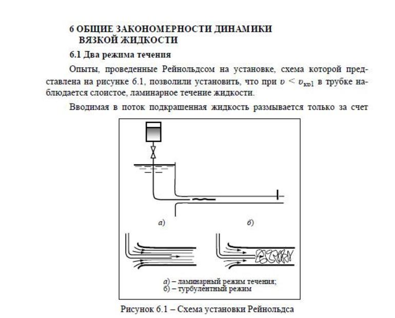
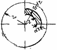
Опыты проводились на специальном лабораторном стенде, который представлял собой заполненный водой бак Б к которому в нижней части присоединена стеклянная трубка Т.

На конце трубки установлен кран К для регулирования расхода жидкости. Расход измеряется с помощью секундомера и мерного бочка М. Бак Б постоянно заполняется водой. Над баком Б расположена ёмкость с краской С. По тонкой трубочке Т1 краска попадает в жидкость, движущуюся в трубке Т. Подачу краски регулирует кран Р.

Опыт №1. Немного приоткрываем кран К. При этом в трубке Т начинается движение жидкости. Открываем кран Р и добавляем в жидкость краску. При небольшой скорости движения в трубке Т краска становится прямолинейной и резко выделяющейся в потоке воды цветной струйкой. Эта струйка не перемешивается с остальной жидкостью. Если ввести в жидкость краску несколькими струйками, то они так и будут двигаться не перемешиваясь с остальной водой.

Движение жидкости, наблюдаемое при малых скоростях, при котором отдельные струйки жидкости движутся параллельно друг другу и оси потока, называют ламинарным (от латинского ламина — слой) или струйчатым движением (режимом). Ламинарное движение может рассматриваться как движение отдельных слоев жидкости, происходящее без перемешивания частиц. Подробнее о ламинарном режиме здесь.

Опыт №2 При намного большем открытии крана струйка краски начинает искривляться и становится волнообразной. Открывая кран ещё больше и увеличивая скорость потока мы увидим, что струйка краски распадается на отдельные вихри и перемешивается с остальной массой воды
Движение жидкости, которое наблюдается при больших скоростях, называется турбулентным (по латински турбулентус — вихревой) движением (режимом). В этом случае в движении жидкости нет видимой закономерности. Отдельные частицы перемешиваются между собой и движутся по самым причудливым, все время меняющимся траекториям весьма сложной формы. Поэтому такое движение называется беспорядочным. Подробнее о турбулентном режиме здесь.

Вывод формулы

Рейнольдс установил, что основными факторами, определяющими характер режима являются:

При этом чем больше размеры поперечного сечения и плотность жидкости и чем меньше её вязкость, тем легче при увеличении скорости осуществить турбулентный режим.

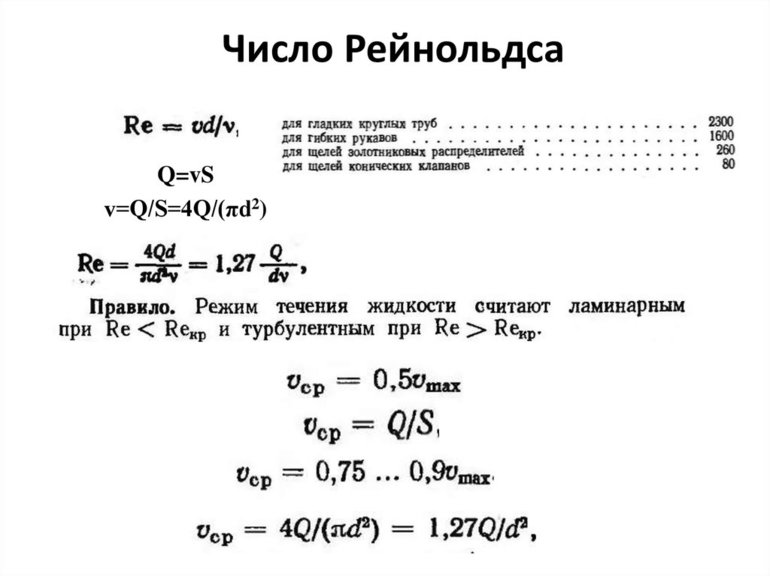
Для характеристики режима движения жидкости Рейнольдсом был выведен безразмерный параметр Re, учитывающий влияние перечисленных выше факторов, называемый число Рейнольдса. Таким образом формула

Re = υ×d× ρ / μ

Поскольку μ / ρ = ν ,
где ν – кинематическая вязкость жидкости, то формула меняет вид на

Re = υ×d / ν

Число Рейнольдса и режимы течения.

Границы существования того или иного режима движения жидкости определяются двумя критическими значениями числа Рейнольдса:

Значение скорости, соответствующее этим значениям Re называют критическими.

При значениях числа Рейнольдса Re < Re_{кр. н.} возможен только ламинарный режим, а при значении Re > Re_{кр. в.} – только турбулентный. При Re_{кр. н.} < Re < Re_{кр. в.} Наблюдается неустойчивое состояние потока. Таким образом, для определения характера режима необходимо в каждом отдельном случае вычислить число Рейнольдса и сопоставить его с критическими значениями этого числа.

В опытах самого известного физика значение числа Рейнольдса Re_кр. было следующим:

Многие эксперименты, проведенные в последствии показали, что критические числа Рейнольдса не являются постоянными величинами и что в действительности при известных условиях неустойчивая зона может оказаться значительно шире.

В настоящее время при практических расчетах обычно принято исходить только из одного критического значения числа Рейнольдса, принимаемого Re_кр =2300, считая, что при Re < 2300 всегда имеет место ламинарный, а при Re > 2300 – всегда турбулентный режимы.

При этом движении жидкости в неустойчивой зоне исключается из особого рассмотрения, это приводит к некоторому запасу и большей надежности в гидравлических расчетах в случае, если в этой зоне действительно имеет место ламинарный режим.

Без особого труда можно получить значения для Reкр для любой формы сечения, а не только круглой формы. Вспоминая, что при круглом сечении радиус

R = d / 4

подставляем в формулу для определения числа Рейнольдса

Re = υ×4×R / ν

Принимая для критического числа Рейнольдса независимо от формы живого сечения величину Re_кр. = 2300, находим, что для сечения любой формы критериев для сужения о характере режима движения является величина, равная 2300 / 4 = 575.

Таким образом, режим ламинарный если значение числа Рейнольдса

И режим турбулентный, если

Видео по теме.

На практике в большинстве случаев (движение воды в трубах, каналах, реках) приходится иметь дело с турбулентным режимом. Ламинарный режим встречается реже. Он наблюдается, например, при движении в трубах очень вязких жидкостей, что иногда имеет место в нефтепроводах, при движении жидкости в очень узких трубках и порах естественных грунтов.

Вместе со статьей «Число Рейнольдса: опыты, формулы и режимы.» смотрят:

Гидростатическое давление: определение, формула и свойства.

Ламинарный режим движения жидкости

Скорость звука, критическая скорость и число Маха

Источник

Содержание

1 Калькулятор для расчета Re онлайн
- 1.1 Расчет по общей формуле
- 1.2 Расчет Re для воды
- 1.3 Расчет Re для воздуха
2 Формула
3 Физический смысл
4 Режимы течения
5 Критическое значение
6 Размерность
7 Течение в трубе

Калькулятор для расчета Re онлайн

Расчет по общей формуле

Расчет Re для воды

Расчет Re для воздуха

Формула

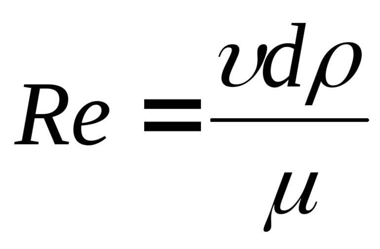
Расчетная формула числа Рейнольдса Re в общем виде:

${mathrm {Re}}={frac {rho vD_{Gamma }}{eta }}={frac {vD_{Gamma }}{nu }}={frac {QD_{Gamma }}{nu A}},$

где

— плотность среды, кг/м³;

— характерная скорость, м/с;

$D_{Gamma }$

— гидравлический диаметр, м;

— динамическая вязкость среды, Па·с или кг/(м·с);

— кинематическая вязкость среды (

), м²/с;

— объёмный расход потока, м³/с;

— площадь сечения канала, например, трубы, м².

Для труб круглого сечения расчетная формула числа Рейнольдса Re будет:

Физический смысл

Физический смысл – число Рейнольдса Re характеризует смену режимов течения от ламинарного к турбулентному. Re является критерием подобия течения вязкой жидкости.

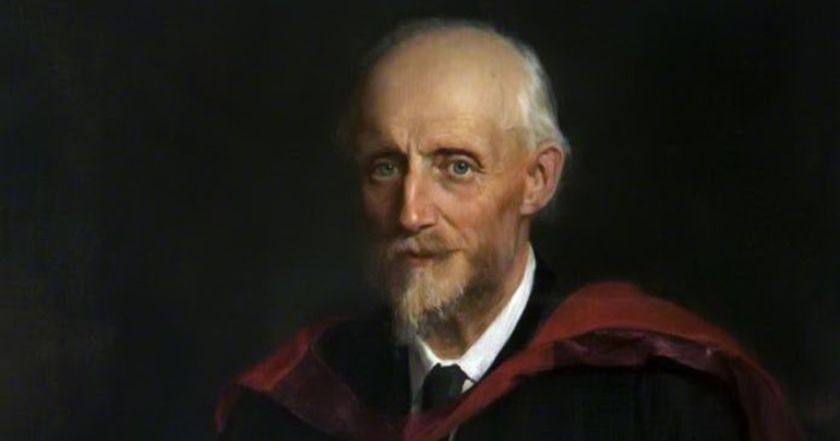
Критерий назван в честь выдающегося английского физика Осборна Рейнольдса (1842—1912).

В настоящее время не существует строгого научно доказанного объяснения этому явлению, однако наиболее достоверной гипотезой считается следующая: смена режимов движения жидкости определяется отношением сил инерции к силам вязкости в потоке жидкости. Если преобладают первые, то режим движения турбулентный, если вторые – ламинарный.

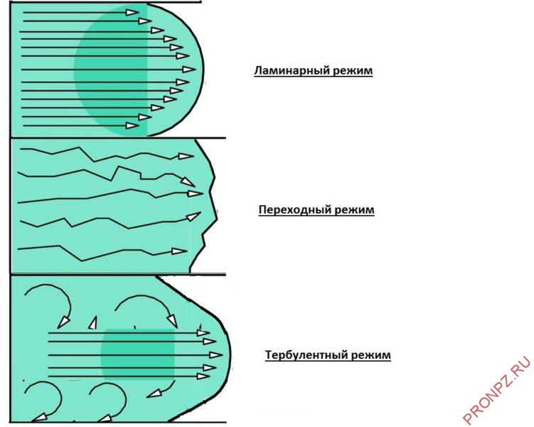
Режимы течения

Режим течения в динамическом пограничном слое зависит от числа Рейнольдса Re и может быть:

Ламинарный режим – слоистое течение без перемешивания частиц жидкости и без пульсации скорости и давления, все линии тока направлены параллельно.
Турбулентный режим – течение, сопровождающееся интенсивным перемешиванием жидкости с пульсациями скоростей и давлений, наряду с основным продольным перемещением жидкости наблюдаются поперечные перемещения и вращательные движения отдельных объемов жидкости.

Эпюры скоростей

Критическое значение

Переход к турбулентному режиму течения жидкости в пограничном слое определяется критическим значением числа Рейнольдса. Это обусловлено тем, что при возрастании скорости, участвующей в расчете числа Re, его значение растет.
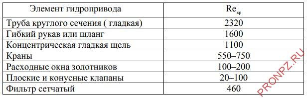
Таким образом, переход от ламинарного режима к турбулентному наблюдается при определенной скорости движения жидкости. Эта скорость называется критической Vкр.

Значение критического числа Re для различных элементов гидропривода

Размерность

Числе Re не имеет единиц измерения. Re является безразмерным критерием подобия течения вязкой жидкости.

Течение в трубе

При ламинарном течении жидкости в прямой трубе или канале постоянного сечения все линии тока направлены параллельно оси трубы, при этом отсутствуют поперечные перемещения частиц жидкости.

При турбулентном течении в канале наряду с основным продольным перемещением жидкости в трубе наблюдаются поперечные перемещения и вращательные движения отдельных объемов жидкости.

Зависимость режима течения от значения числа Re в гладких трубах:

<2100 – Ламинарный режим
2100 – 2300 – Переходный режим
>2300 – Турбулентный режим

Обычно предполагается, что при числе Re выше 2300 образуется турбулентный режим.

Тем не менее, при значениях Re выше критического и до определённого предела наблюдается переходной (смешанный) режим течения жидкости, когда турбулентное течение более вероятно, но ламинарное в некоторых конкретных случаях тоже наблюдается — так называемая неустойчивая турбулентность. В трубах такой переходный интервал может достигать вплоть до Re = 2300—10 000.

Источник

Опыты Рейнольдса

Рейнольдс проводил эксперименты на установке, представлявшей собой бак с водой, к которому в нижней части была присоединена выходная стеклянная трубка с краном на конце. Бак постоянно наполнялся водой, а расход воды мерился при помощи мерного бачка и секундомера. Над баком находился сосуд с краской, которая попадала в воду по тонкой трубочке с краном.

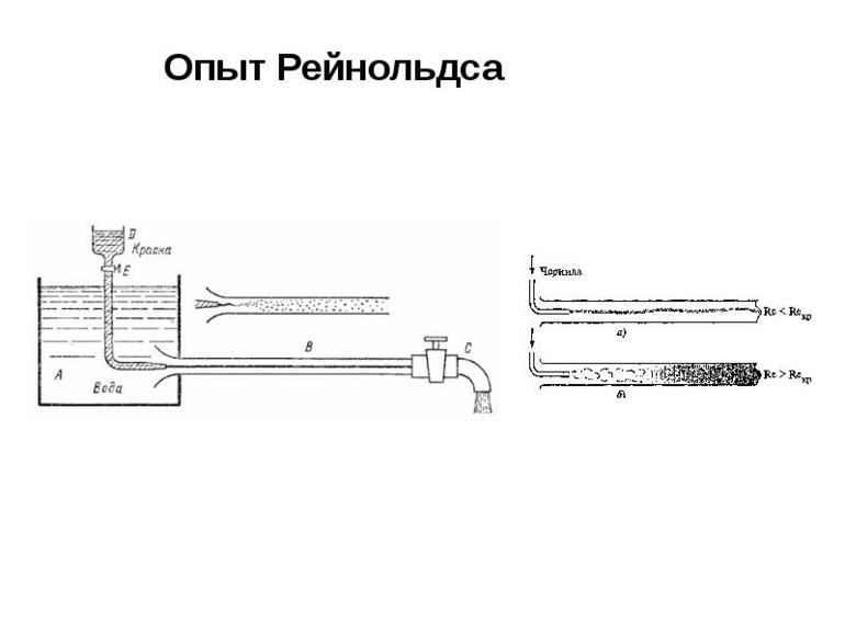
Первый опыт. Немного приоткрывался кран на выходе из бака и в трубке начиналось движение воды при небольшой скорости. При добавлении краски в выходной трубке появлялась резко очерченная цветная струйка, которая не смешивалась с остальной водой. Фиксировался ламинарный режим течения.
Второй опыт. При дальнейшем открывании крана и увеличении скорости потока струйка краски начинала изгибаться, превращалась в отдельные вихри и перемешивалась с остальной водой. Ламинарный режим переходил в турбулентный.

Рейнольдс доказал, что при значении числа Re 2000—3000 поток становится турбулентным, а при Re меньше нескольких сотен — поток полностью ламинарный.

Режимы течения жидкости

Опыты, проводившиеся Рейнольдсом, подтвердили наличие двух режимов течения жидкости — турбулентного и ламинарного. Учёный сформулировал общие условия существования режимов и переходного состояния между ними. Разные жидкости при протекании по трубам, обтекании преград или растекании по поверхности демонстрируют различные свойства. Густая липкая жидкость, например, клей, обладает большей вязкостью, чем лёгкая и подвижная вода. Степень вязкости определяется коэффициентом динамической вязкости η («эта»). Для ламинарного потока свойственны следующие признаки:

Отсутствует смешивание отдельных слоёв.
Слои, расположенные ближе к оси трубы, перемещаются быстрее, чем находящиеся у стенок. Этот объясняется силами трения, возникающими между молекулами жидкости и внутренней поверхностью трубы.

Турбулентное течение — хаотический поток, каждая молекула которого двигается произвольно по непредсказуемой траектории. При этом в потоке образуются завихрения. Но, несмотря на хаотичность перемещения частиц, общий гидравлический поток имеет направление и скорость, которая оценивается по средним значениям. В большей части поперечного сечения скорость только немного меньше максимальной, но вблизи стенок она резко падает.

Рейнольдс провёл значительное количество опытов с разными жидкостями для определения числа, безразмерная величина которого описывает характер гидравлического потока. Это число имеет обозначение Re. Экспериментально было установлено, что при превышении числом Рейнольдса критической величины наблюдается переход движения жидкости, текущей в трубе, из ламинарного режима в турбулентный.

Число Рейнольдса характеризует режим движения и даёт правильные значения при расчёте для напорных потоков. В потоках без напора переходный период увеличивается, и использование Re в качестве критерия не всегда подходит. Например, в водохранилищах значения велики, но там происходит ламинарное течение.

Скорость среды

Скорость, при которой изменяется режим потока — критическая. Существует 2 вида: одна соответствует переходу от ламинарного течения к турбулентному и другая, соответствующая обратному переходу от турбулентного к ламинарному. Между этими значениями может наблюдаться как один, так и другой режим. Этот период определяется как переходный. Для случая движения жидкости в трубопроводе Рейнольдс назвал следующие параметры, от которых зависит режим гидравлического потока:

диаметр трубопровода — d;
средняя скорость течения — V;
плотность жидкости — ρ;
динамическая вязкость жидкости — η.

При этом лёгкость осуществления турбулентного режима прямо пропорциональна поперечному сечению трубы и плотности и обратно пропорциональна вязкости. Формула числа Рейнольдса:

Re = V d ρ / η;

Подставляя в эту формулу соответствующие параметры скорости среды, её плотности, вязкости и размеры трубы, можно произвести расчёт значения числа Re и определить режим потока. Число Re не имеет размерности. Это становится понятно, если подставить в формулу все параметры со своими единицами измерения. В результате сокращения получается безразмерное число. Для гидравлического потока в прямой круглой трубе с гладкими стенками критическое значение Re в норме равно 2100—2300. Анализ показывает, что критическое значение числа Re возрастает в сужающихся трубопроводах и снижается в расширяющихся.

При расчётах обычно принимают только одно критическое значение числа Re. Предполагается, что Re < 2300 соответствует ламинарному режиму, а Re > 2300 — турбулентному. Течение жидкости в переходной зоне не рассматривается. Это обеспечивает некоторый запас и увеличивает надёжность расчётов. Для газов Re критическое достигается при значительно больших скоростях течения, чем у жидкостей, так как у них намного больше кинематическая вязкость (ν = η / ρ).

Турбулентное движение наблюдается чаще, чем ламинарное. Скорости при хаотичном движении более равномерно распределены по сечению потока. Это происходит в связи с перемешиванием молекул с разными скоростями и уравниванием средней скорости по всему поперечному сечению. Ламинарные потоки наблюдается при движении вязких жидкостей по трубам, в течении грунтовых вод и крови в живых организмах.

Значение числа Re

Жидкость в гидравлическом потоке имеет инерцию и пытается поддерживать имеющуюся скорость. При большой вязкости среды внутреннее трение между слоями оказывает значительное сопротивление. Число Re зависит от соотношения между силами инерции и трения. Большие значения Re соответствуют случаю, когда сопротивление трения мало и не может загасить турбулентность. Малые величины Re относятся к обстоятельствам, когда трение уменьшает турбулентность и превращает гидравлический поток в ламинарный.

Физический смысл числа Рейнольдса — отношение сил инерции потока к силам вязкости. Можно говорить, что это соотношение выражает зависимость между кинетической энергией потока и тепловыми потерями энергии на трение при аналогичной длине.

Число Рейнольдса используется при моделировании потоков в различных газах и жидкостях, так как режим течения зависит только от соотношения физических величин: плотности, вязкости, скорости и размеров элемента, которое выражается числом Re, поэтому можно использовать для эксперимента в аэродинамической трубе уменьшенный прототип летательного аппарата и выбрать скорость потока воздуха так, чтобы число Рейнольдса соответствовало реальному для аппарата в полёте. Сейчас нет необходимости в использовании аэродинамической трубы. Все воздушные потоки можно моделировать с помощью компьютера.

Рейнольдс внёс большой вклад в гидравлику, гидродинамику и механику. Он представил дифференциальные уравнения осреднённого движения жидкости, учитывающие турбулентные напряжения, создал труды по теории смазки, определил критерий подобия двух различных течений, исследовал явления кавитации на примере винтовой лопасти, модернизировал устройство центробежных насосов. В 1888 году он был награждён медалью Лондонского королевского общества.

Источник

Рассм.
нек. трубу в которой протекает жидкость.Если
будет иметь месть переход от одного
режима к другому, то он будет
происходить примерно при одной и той
же скорости, которую называют критической
скоростью и обозначают V_кр.
значение этой скорости прямо
пропорционально кинематическому
коэффициенту вязкости жидкости

и обратно пропорционально диаметру
трубопровода d
или
гидравлическому радиусу потока R

к-
безразмер.
величина,
одинакова
для всех жидкостей для любых размеров
труб и сечений потока. Безразм.
коэф.

наз.
критическим числом Рейнольдса.

Опытным путём установлено, что критическое
число Рейнольдса для круглых труб —
2320 для круглых труб, а для других сечений
580.

Для
определения режима движения в потоке
надо найти фактическое число Рейнольдса
Re
, которое можно установить для любого
потока по формуле

и
сравнить его с критическим числом Re_кр_.При
этом, если Re

Re_кр,
то режим движения ламинарный, если Re
> Re_кр,
то режим движения турбулентный.

29!.Понятие пульсационной, мгновенной, осреднённой и сред.Скоростей

Отличительной
особенностью турбулентного движения
жидкости является хаотическое движение
частиц в потоке.

(1)

Однако
при этом можно наблюдать и некоторую
закономерность в таком движении. С
помощью прибора позволяющего фиксировать
изменение скорости в точке замера, можно
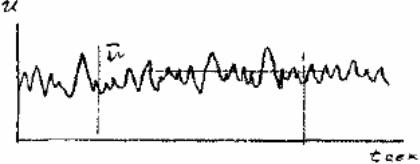
снять кривую скорости.Величина скорости
в данной точке в данный момент времени
носит название мгновенной скорости.
График изменения мгновенной скорости
во времени u(t) представлена
на рис.
Если выбрать на кривой скоростей
некоторый интервал времени и провести
интегрирование кривой скоростей, а
затем найти среднюю величину, то такая
величина носит название осреднённой
скорости
:(1).Разница
между мнгновенной и осреднённой скоростью
называется скоростью пульсации и’.

Если
величины осреднённых скоростей в
различные интервалы времени будут
оставаться постоянными, то такое
турбулентное движение жидкости будет
установившемся. При неустанов.
турб.
движении жидкости величины осреднённых
скоростей меняются во времени.Пульсация
жидкости является причиной перемешив.
жидкости в потоке. Интенсивность перемеш.
Зависит от
числа Rе,
т.е. при сохр.
прочих условий от скорости движения
жидкости. Таким образом
в потоке жидкости
характер её движения зависит от скорости.
Увеличение скорости до критического
значения приведёт к смене режима движения
с ламинарного на турбулентный режим.

Средней
скоростью-фиктивная
скорость, с
которой
должны двигаться все частицы жидкости
в данном живом сечения,чтобы расход
жидкости, проходящей с этой скоростью
через сечение,

оставался
равным расходу, вычисленному по
действительным скоростям
всех
частиц в сечении.

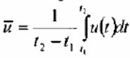
29.Ламинарн.Режим.Распредел.Скорости ж-ти по сечению потока.Определ.Расхода ж-ти и средней скор.Ломин.Потока

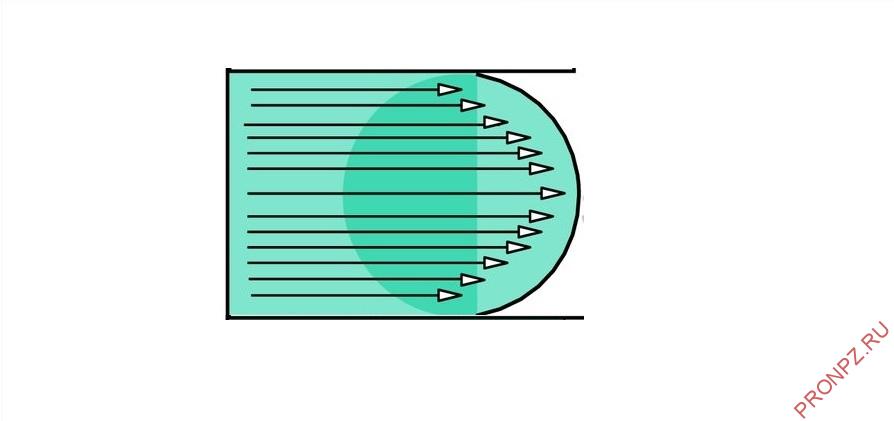
Распределение
скоростей в ламинарном потоке. Поскольку
ламинарный поток жидкости в круглой
цилиндрической трубе является осе
симметричным, рассмотрим, как и ранее,
лишь одно (вертикальное сечение трубы).
Тогда, согласно гипотезе Ньютона:

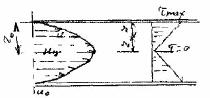
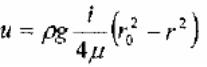
Отсюда
видно, что распределение скоростей в
круглой цилиндрической трубе соответствует
параболическому закону. Максимальная
величина скорости будет в центре трубы,
где= О.

Средняя
скорость движения жидкости в ламинарном
потоке. Для определения
величины средней скорости рассмотрим
живое сечение потока жидкости в трубе
Затем проведём в сечении потока две
концентрические окружности, отстоящие
друг от друга на бесконечно малое
расстояние dr. Между
этими окружностями мы, таким образом,
выделили малую кольцевую зону, малую
часть живого сечения потока жидкости.
Расход жидкости через выделенную
кольцевую зону:

Расход
жидк.
через
полное живое
сечение
трубы: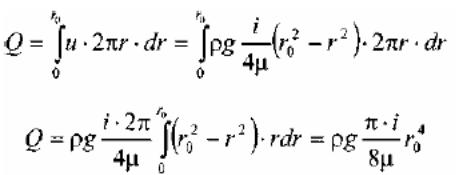

величина
средней скорости в сечении:.

Соседние файлы в предмете [НЕСОРТИРОВАННОЕ]

Источник

Definition[edit]

History[edit]

Flow in a pipe[edit]

Laminar–turbulent transition[edit]

Flow in a wide duct[edit]

Flow in an open channel[edit]

Flow around airfoils[edit]

Object in a fluid[edit]

In viscous fluids[edit]

Sphere in a fluid[edit]

Rectangular object in a fluid[edit]

Fall velocity[edit]

Packed bed[edit]

Stirred vessel[edit]

Pipe friction[edit]

Similarity of flows[edit]

Smallest scales of turbulent motion[edit]

In physiology[edit]

Complex systems[edit]

Derivation[edit]

Relationship to other dimensionless parameters[edit]

See also[edit]

References[edit]

Footnotes[edit]

Citations[edit]

Sources[edit]

Further reading[edit]

External links[edit]

Число Рейнольдса

Опыты Рейнольдса

Вывод формулы

Число Рейнольдса и режимы течения.

Видео по теме.

Калькулятор для расчета Re онлайн

Расчет по общей формуле

Расчет Re для воды

Расчет Re для воздуха

Формула

Физический смысл

Режимы течения

Критическое значение

Размерность

Течение в трубе

Опыты Рейнольдса

Режимы течения жидкости

Скорость среды

Значение числа Re

29!.Понятие пульсационной, мгновенной, осреднённой и сред.Скоростей

29.Ламинарн.Режим.Распредел.Скорости ж-ти по сечению потока.Определ.Расхода ж-ти и средней скор.Ломин.Потока