UCHEES.RU — помощь студентам и школьникам
В 15:47 поступил вопрос в раздел ЕГЭ (школьный), который вызвал затруднения у обучающегося.
Вопрос вызвавший трудности
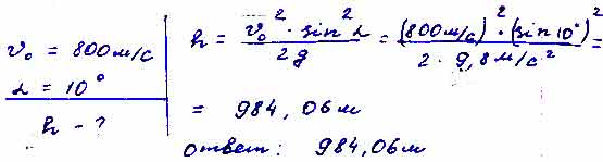
Определите максимальную высоту полёта снаряда, выпущенного из пушки со скоростью 800 м/с под углом 10° к горизонту.
Ответ подготовленный экспертами Учись.Ru
Для того чтобы дать полноценный ответ, был привлечен специалист, который хорошо разбирается требуемой тематике «ЕГЭ (школьный)». Ваш вопрос звучал следующим образом: Определите максимальную высоту полёта снаряда, выпущенного из пушки со скоростью 800 м/с под углом 10° к горизонту.
После проведенного совещания с другими специалистами нашего сервиса, мы склонны полагать, что правильный ответ на заданный вами вопрос будет звучать следующим образом:
ответ к заданию по физике
НЕСКОЛЬКО СЛОВ ОБ АВТОРЕ ЭТОГО ОТВЕТА:

Работы, которые я готовлю для студентов, преподаватели всегда оценивают на отлично. Я занимаюсь написанием студенческих работ уже более 4-х лет. За это время, мне еще ни разу не возвращали выполненную работу на доработку! Если вы желаете заказать у меня помощь оставьте заявку на этом сайте. Ознакомиться с отзывами моих клиентов можно на этой странице.
Миронова Любовь Романовна — автор студенческих работ, заработанная сумма за прошлый месяц 84 300 рублей. Её работа началась с того, что она просто откликнулась на эту вакансию
ПОМОГАЕМ УЧИТЬСЯ НА ОТЛИЧНО!
Выполняем ученические работы любой сложности на заказ. Гарантируем низкие цены и высокое качество.
![]()
Деятельность компании в цифрах:
Зачтено оказывает услуги помощи студентам с 1999 года. За все время деятельности мы выполнили более 400 тысяч работ. Написанные нами работы все были успешно защищены и сданы. К настоящему моменту наши офисы работают в 40 городах.
РАЗДЕЛЫ САЙТА
Ответы на вопросы — в этот раздел попадают вопросы, которые задают нам посетители нашего сайта. Рубрику ведут эксперты различных научных отраслей.
Полезные статьи — раздел наполняется студенческой информацией, которая может помочь в сдаче экзаменов и сессий, а так же при написании различных учебных работ.
Красивые высказывания — цитаты, афоризмы, статусы для социальных сетей. Мы собрали полный сборник высказываний всех народов мира и отсортировали его по соответствующим рубрикам. Вы можете свободно поделиться любой цитатой с нашего сайта в социальных сетях без предварительного уведомления администрации.
ЗАДАТЬ ВОПРОС
НОВЫЕ ОТВЕТЫ
- Абадзехская стоянка, Даховская пещера. ..
- По закону сохранения заряда каждый шарик после соприкасl..
- 2)прогудел первый мохнатый шмель 3) Зазвенела Прогудел 4) ..
- В мілкій траві ворушаться сліди веселих, сполоханих доще
..
ПОХОЖИЕ ВОПРОСЫ
- Из-под колёс буксующего автомобиля вылетают комья грязи и падают на разных расстояниях от него, при этом максимальное расстояние составля…
- По дороге со скоростью 72 км/ч едут два автомобиля: грузовой, а за ним легковой. С заднего колеса грузового автомобиля срывается камень. На ка
- При езде на велосипеде без заднего щитка грязь с колёс может попасть на спину велосипедисту. Объясните с точки зрения физики, почему это пр…
- Теннисист при подаче запускает мяч с высоты 2 м над землёй. На каком расстоянии от подающего мяч ударится о корт, если начальная скорость мя…
Площадка Учись.Ru разработана специально для студентов и школьников. Здесь можно найти ответы на вопросы по гуманитарным, техническим, естественным, общественным, прикладным и прочим наукам. Если же ответ не удается найти, то можно задать свой вопрос экспертам. С нами сотрудничают преподаватели школ, колледжей, университетов, которые с радостью помогут вам. Помощь студентам и школьникам оказывается круглосуточно. С Учись.Ru обучение станет в несколько раз проще, так как здесь можно не только получить ответ на свой вопрос, но расширить свои знания изучая ответы экспертов по различным направлениям науки.
2020 — 2023 — UCHEES.RU
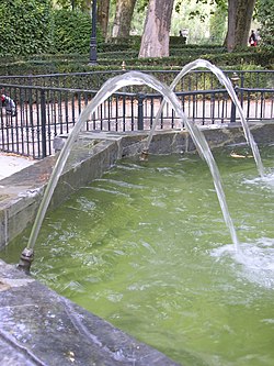
Parabolic water motion trajectory
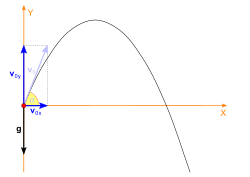
Components of initial velocity of parabolic throwing

Ballistic trajectories are parabolic if gravity is homogeneous and elliptic if it is round.
Projectile motion is a form of motion experienced by an object or particle (a projectile) that is projected in a gravitational field, such as from Earth’s surface, and moves along a curved path under the action of gravity only. In the particular case of projectile motion on Earth, most calculations assume the effects of air resistance are passive and negligible. The curved path of objects in projectile motion was shown by Galileo to be a parabola, but may also be a straight line in the special case when it is thrown directly upward or downward. The study of such motions is called ballistics, and such a trajectory is a ballistic trajectory. The only force of mathematical significance that is actively exerted on the object is gravity, which acts downward, thus imparting to the object a downward acceleration towards the Earth’s center of mass. Because of the object’s inertia, no external force is needed to maintain the horizontal velocity component of the object’s motion. Taking other forces into account, such as aerodynamic drag or internal propulsion (such as in a rocket), requires additional analysis. A ballistic missile is a missile only guided during the relatively brief initial powered phase of flight, and whose remaining course is governed by the laws of classical mechanics.
Ballistics (from Ancient Greek βάλλειν bállein ‘to throw’) is the science of dynamics that deals with the flight, behavior and effects of projectiles, especially bullets, unguided bombs, rockets, or the like; the science or art of designing and accelerating projectiles so as to achieve a desired performance.

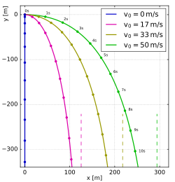
Trajectories of a projectile with air drag and varying initial velocities
The elementary equation of ballistics neglect nearly every factor except for initial velocity and an assumed constant gravitational acceleration. Practical solutions of a ballistics problem often require considerations of air resistance, cross winds, target motion, varying acceleration due to gravity, and in such problems as launching a rocket from one point on the Earth to another, the rotation of the Earth. Detailed mathematical solutions of practical problems typically do not have closed-form solutions, and therefore require numerical methods to address.
Kinematic quantities[edit]
In projectile motion, the horizontal motion and the vertical motion are independent of each other; that is, neither motion affects the other. This is the principle of compound motion established by Galileo in 1638,[1] and used by him to prove the parabolic form of projectile motion.[2]
The horizontal and vertical components of a projectile’s velocity are independent of each other.
A ballistic trajectory is a parabola with homogeneous acceleration, such as in a space ship with constant acceleration in absence of other forces. On Earth the acceleration changes magnitude with altitude and direction with latitude/longitude. This causes an elliptic trajectory, which is very close to a parabola on a small scale. However, if an object was thrown and the Earth was suddenly replaced with a black hole of equal mass, it would become obvious that the ballistic trajectory is part of an elliptic orbit around that black hole, and not a parabola that extends to infinity. At higher speeds the trajectory can also be circular, parabolic or hyperbolic (unless distorted by other objects like the Moon or the Sun). In this article a homogeneous acceleration is assumed.
Acceleration[edit]
Since there is acceleration only in the vertical direction, the velocity in the horizontal direction is constant, being equal to  . The vertical motion of the projectile is the motion of a particle during its free fall. Here the acceleration is constant, being equal to g.[note 1] The components of the acceleration are:
 ,
,- .


Velocity[edit]
Let the projectile be launched with an initial velocity  , which can be expressed as the sum of horizontal and vertical components as follows:
- .

The components  and
and  can be found if the initial launch angle,
  , is known:
- ,


The horizontal component of the velocity of the object remains unchanged throughout the motion. The vertical component of the velocity changes linearly,[note 2] because the acceleration due to gravity is constant. The accelerations in the x and y directions can be integrated to solve for the components of velocity at any time t, as follows:
- ,
- .


The magnitude of the velocity (under the Pythagorean theorem, also known as the triangle law):
- .

Displacement[edit]
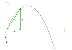
Displacement and coordinates of parabolic throwing
At any time  , the projectile’s horizontal and vertical displacement are:
- ,
- .

The magnitude of the displacement is:
- .

Consider the equations,
- .

If t is eliminated between these two equations the following equation is obtained:

Here R is the Range of a projectile.
Since g, θ, and v0 are constants, the above equation is of the form
- ,

in which a and b are constants. This is the equation of a parabola, so the path is parabolic. The axis of the parabola is vertical.
If the projectile’s position (x,y) and launch angle (θ or α) are known, the initial velocity can be found solving for v0 in the aforementioned parabolic equation:
- .

Displacement in polar coordinates[edit]
The parabolic trajectory of a projectile can also be expressed in polar coordinates instead of Cartesian coordinates. In this case, the position has the general formula
- .

In this equation, the origin is the midpoint of the horizontal range of the projectile, and if the ground is flat, the parabolic arc is plotted in the range  . This expression can be obtained by transforming the Cartesian equation as stated above by
  and
and  .
.
Properties of the trajectory[edit]
Time of flight or total time of the whole journey[edit]
The total time t for which the projectile remains in the air is called the time of flight.
After the flight, the projectile returns to the horizontal axis (x-axis), so  .
.


Note that we have neglected air resistance on the projectile.
If the starting point is at height y0 with respect to the point of impact, the time of flight is:

As above, this expression can be reduced to

if θ is 45° and y0 is 0.
Time of flight to the target’s position[edit]
As shown above in the Displacement section, the horizontal and vertical velocity of a projectile are independent of each other.
Because of this, we can find the time to reach a target using the displacement formula for the horizontal velocity:


This equation will give the total time t the projectile must travel for to reach the target’s horizontal displacement, neglecting air resistance.
Maximum height of projectile[edit]

Maximum height of projectile
The greatest height that the object will reach is known as the peak of the object’s motion.
The increase in height will last until  , that is,
- .

Time to reach the maximum height(h):
- .

For the vertical displacement of the maximum height of projectile:


The maximum reachable height is obtained for θ=90°:

If the projectile’s position (x,y) and launch angle (θ) are known, the maximum height can be found solving for h in the following equation:

Relation between horizontal range and maximum height[edit]
The relation between the range d on the horizontal plane and the maximum height h reached at  is:
is:

Maximum distance of projectile[edit]
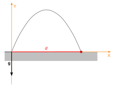
The maximum distance of projectile
The range and the maximum height of the projectile does not depend upon its mass. Hence range and maximum height are equal for all bodies that are thrown with the same velocity and direction.
The horizontal range d of the projectile is the horizontal distance it has traveled when it returns to its initial height ().
- .

Time to reach ground:
- .

From the horizontal displacement the maximum distance of projectile:
- ,

so[note 3]
- .

Note that d has its maximum value when
- ,

which necessarily corresponds to
- ,

or
- .


Trajectories of projectiles launched at different elevation angles but the same speed of 10 m/s in a vacuum and uniform downward gravity field of 10 m/s2. Points are at 0.05 s intervals and length of their tails is linearly proportional to their speed. t = time from launch, T = time of flight, R = range and H = highest point of trajectory (indicated with arrows).
The total horizontal distance (d) traveled.

When the surface is flat (initial height of the object is zero), the distance traveled:[3]

Thus the maximum distance is obtained if θ is 45 degrees. This distance is:

Application of the work energy theorem[edit]
According to the work-energy theorem the vertical component of velocity is:
- .

These formulae ignore aerodynamic drag and also assume that the landing area is at uniform height 0.
Angle of reach[edit]
The «angle of reach» is the angle (θ) at which a projectile must be launched in order to go a distance d, given the initial velocity v.

There are two solutions:
- (shallow trajectory)

and
- (steep trajectory)

Angle θ required to hit coordinate (x, y)[edit]

Vacuum trajectory of a projectile for different launch angles. Launch speed is the same for all angles, 50 m/s if «g» is 10 m/s2.
To hit a target at range x and altitude y when fired from (0,0) and with initial speed v the required angle(s) of launch θ are:

The two roots of the equation correspond to the two possible launch angles, so long as they aren’t imaginary, in which case the initial speed is not great enough to reach the point (x,y) selected. This formula allows one to find the angle of launch needed without the restriction of .
One can also ask what launch angle allows the lowest possible launch velocity. This occurs when the two solutions above are equal, implying that the quantity under the square root sign is zero. This requires solving a quadratic equation for  , and we find

This gives

If we denote the angle whose tangent is y/x by α, then


This implies

In other words, the launch should be at the angle halfway between the target and Zenith (vector opposite to Gravity)
Total Path Length of the Trajectory[edit]
The length of the parabolic arc traced by a projectile L, given that the height of launch and landing is the same and that there is no air resistance, is given by the formula:

where  is the initial velocity, is the launch angle and
  is the acceleration due to gravity as a positive value. The expression can be obtained by evaluating the arc length integral for the height-distance parabola between the bounds initial and final displacements (i.e. between 0 and the horizontal range of the projectile) such that:
- .

Trajectory of a projectile with air resistance[edit]
Air resistance creates a force that (for symmetric projectiles) is always directed against the direction of motion in the surrounding medium and has a magnitude that depends on the absolute speed:  . The speed-dependence of the friction force is linear (
 ) at very low speeds (Stokes drag) and quadratic (
 ) at larger speeds (Newton drag).[4] The transition between these behaviours is determined by the Reynolds number, which depends on speed, object size and kinematic viscosity of the medium. For Reynolds numbers below about 1000, the dependence is linear, above it becomes quadratic. In air, which has a kinematic viscosity around
  , this means that the drag force becomes quadratic in v when the product of speed and diameter is more than about
  , which is typically the case for projectiles.
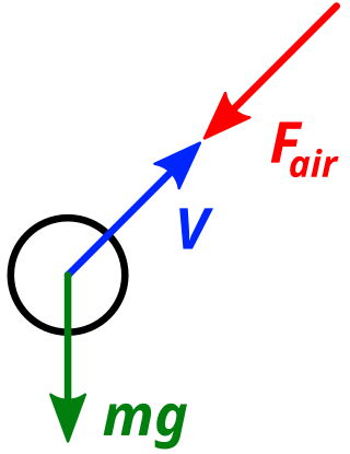
Free body diagram of a body on which only gravity and air resistance acts
The free body diagram on the right is for a projectile that experiences air resistance and the effects of gravity. Here, air resistance is assumed to be in the direction opposite of the projectile’s velocity: 
Trajectory of a projectile with Stokes drag[edit]
Stokes drag, where  , only applies at very low speed in air, and is thus not the typical case for projectiles. However, the linear dependence of
  on
on  causes a very simple differential equation of motion

in which the two cartesian components become completely independent, and thus easier to solve.[5]
Here, , and
and  will be used to denote the initial velocity, the velocity along the direction of x and the velocity along the direction of y, respectively. The mass of the projectile will be denoted by m, and
  . For the derivation only the case where
  is considered. Again, the projectile is fired from the origin (0,0).
|
Derivation of horizontal position |
|---|
|
The relationships that represent the motion of the particle are derived by Newton’s Second Law, both in the x and y directions. This implies that:
and
Solving (1) is an elementary differential equation, thus the steps leading to a unique solution for vx and, subsequently, x will not be enumerated. Given the initial conditions
|


- (1b)

|
Derivation of vertical position |
|---|
|
While (1) is solved much in the same way, (2) is of distinct interest because of its non-homogeneous nature. Hence, we will be extensively solving (2). Note that in this case the initial conditions are used
This first order, linear, non-homogeneous differential equation may be solved a number of ways; however, in this instance, it will be quicker to approach the solution via an integrating factor
And by integration we find:
Solving for our initial conditions:
With a bit of algebra to simplify (3a): |


- (3b)

- .

Trajectory of a projectile with Newton drag[edit]
Trajectories of a skydiver in air with Newton drag
The most typical case of air resistance, for the case of Reynolds numbers above about 1000 is Newton drag with a drag force proportional to the speed squared,  . In air, which has a kinematic viscosity around , this means that the product of speed and diameter must be more than about .
Unfortunately, the equations of motion can not be easily solved analytically for this case. Therefore, a numerical solution will be examined.
The following assumptions are made:
- Constant gravitational acceleration
- Air resistance is given by the following drag formula,

-
- Where:
-
-
- FD is the drag force
- c is the drag coefficient
- ρ is the air density
- A is the cross sectional area of the projectile
- μ = k/m = cρA/(2m)
-
Special cases[edit]
Even though the general case of a projectile with Newton drag cannot be solved analytically, some special cases can. Here we denote the terminal velocity in free-fall as  and the characteristic settling time constant
  .
.
- Near-horizontal motion: In case the motion is almost horizontal, , such as a flying bullet, the vertical velocity component has very little influence on the horizontal motion. In this case:[7]

-
- The same pattern applies for motion with friction along a line in any direction, when gravity is negligible. It also applies when vertical motion is prevented, such as for a moving car with its engine off.


- Vertical motion upward:[7]
-
- Here
- and
- where is the initial upward velocity at and the initial position is .
- A projectile can not rise longer than vertically before it reaches the peak.


- Vertical motion downward:[7]
-
- After a time , the projectile reaches almost terminal velocity .


Numerical solution[edit]
A projectile motion with drag can be computed generically by numerical integration of the ordinary differential equation, for instance by applying a reduction to a first-order system. The equation to be solved is
- .

This approach also allows to add the effects of speed-dependent drag coefficient, altitude-dependent air density and position-dependent gravity field.
Lofted trajectory[edit]

A special case of a ballistic trajectory for a rocket is a lofted trajectory, a trajectory with an apogee greater than the minimum-energy trajectory to the same range. In other words, the rocket travels higher and by doing so it uses more energy to get to the same landing point. This may be done for various reasons such as increasing distance to the horizon to give greater viewing/communication range or for changing the angle with which a missile will impact on landing. Lofted trajectories are sometimes used in both missile rocketry and in spaceflight.[8]
Projectile motion on a planetary scale[edit]

Projectile trajectory around a planet, compared to the motion in a uniform field
When a projectile without air resistance travels a range that is significant compared to the earth’s radius (above ≈100 km), the curvature of the earth and the non-uniform Earth’s gravity have to be considered. This is for example the case with spacecraft or intercontinental projectiles. The trajectory then generalizes from a parabola to a Kepler-ellipse with one focus at the center of the earth. The projectile motion then follows Kepler’s laws of planetary motion.
The trajectories’ parameters have to be adapted from the values of a uniform gravity field stated above. The earth radius is taken as R, and g as the standard surface gravity. Let  the launch velocity relative to the first cosmic velocity.
Total range d between launch and impact:

Maximum range of a projectile for optimum launch angle ( ):
):
- with , the first cosmic velocity


Maximum height of a projectile above the planetary surface:

Maximum height of a projectile for vertical launch ( ):
):
- with , the second cosmic velocity


Time of flight:

See also[edit]
- Equations of motion
Notes[edit]
References[edit]
- ^ Galileo Galilei, Two New Sciences, Leiden, 1638, p.249
- ^ Nolte, David D., Galileo Unbound (Oxford University Press, 2018) pp. 39-63.
- ^ Tatum (2019). Classical Mechanics (PDF). pp. ch. 7.
- ^ Stephen T. Thornton; Jerry B. Marion (2007). Classical Dynamics of Particles and Systems. Brooks/Cole. p. 59. ISBN 978-0-495-55610-7.
- ^ Atam P. Arya; Atam Parkash Arya (September 1997). Introduction to Classical Mechanics. Prentice Hall Internat. p. 227. ISBN 978-0-13-906686-3.
- ^ Rginald Cristian, Bernardo; Jose Perico, Esguerra; Jazmine Day, Vallejos; Jeff Jerard, Canda (2015). «Wind-influenced projectile motion». European Journal of Physics. 36 (2): 025016. Bibcode:2015EJPh…36b5016B. doi:10.1088/0143-0807/36/2/025016. S2CID 119601402.
- ^ a b c Walter Greiner (2004). Classical Mechanics: Point Particles and Relativity. Springer Science & Business Media. p. 181. ISBN 0-387-95586-0.
- ^ Ballistic Missile Defense, Glossary, v. 3.0, US Department of Defense, June 1997.

hmax — максимальная высота
Smax — максимальная дальность полета, если бросок и падение на одном уровне
Sh — расстояние пройденное по горизонтали до момента максимального подъема
tmax — время всего полета
th — время за которое тело поднялось на максимальную высоту
Vo — начальная скорость тела
α — угол под которым брошено тело
g ≈ 9,8 м/с2 — ускорение свободного падения
Формула для расчета максимальной высоты достигнутое телом, если даны, начальная скорость Vo и угол α под которым брошено тело. :

Формула для вычисления максимальной высоты, если известны, максимальное расстояние S max или расстояние по горизонтали при максимальной высоте Sh и угол α под которым брошено тело. :

По этой формуле, можно определить максимальную высоту, если известно время th за которое тело поднялось на эту высоту. :

Формула для расчета максимальной дальности полета, если даны, начальная скорость броска Vo и угол α под которым брошено тело. :

или известны максимальная высота hmax и угол α под которым брошено тело. :

Формула для нахождения расстояния по горизонтали при максимальной высоте, если даны, начальная скорость броска Vo и угол α под которым брошено тело. :

или известны максимальная высота hmax и угол α под которым брошено тело. :

* т. к. траектория движения симметрична относительно линии максимальной высоты, то расстояние Sh ровно в два раза, меньше максимальной дальности броска Smax
Формула для определения времени затраченного на весь полет, если даны, начальная скорость Vo и угол α под которым брошено тело или если известна только максимальная высота hmax :

* т. к. траектория движения симметрична относительно линии максимальной высоты, то время максимального подъема th ровно в два раза, меньше максимального времени tmax
Формула для определения времени за которое тело поднялось на максимальную высоту, если даны, начальная скорость Vo и угол α под которым брошено тело или если известна только максимальная высота hmax :

- Подробности
-
Опубликовано: 11 августа 2015
-
Обновлено: 13 августа 2021
Моделирование динамических систем: решение нелинейных уравнений
Время на прочтение
8 мин
Количество просмотров 11K
Введение
Конечной целью математического моделирования в любой области знаний является получение количественных характеристик исследуемого объекта. Некоторые параметры пушки, стрельбу из которой мы моделировали в прошлый раз, были заданы в условии задачи: начальная скорость снаряда, его калибр и материал, из которого он изготовлен. Угол наклона ствола можно отнести к варьируемым параметрам: любое серьезное орудие допускает наводку, в том числе и в вертикальной плоскости.

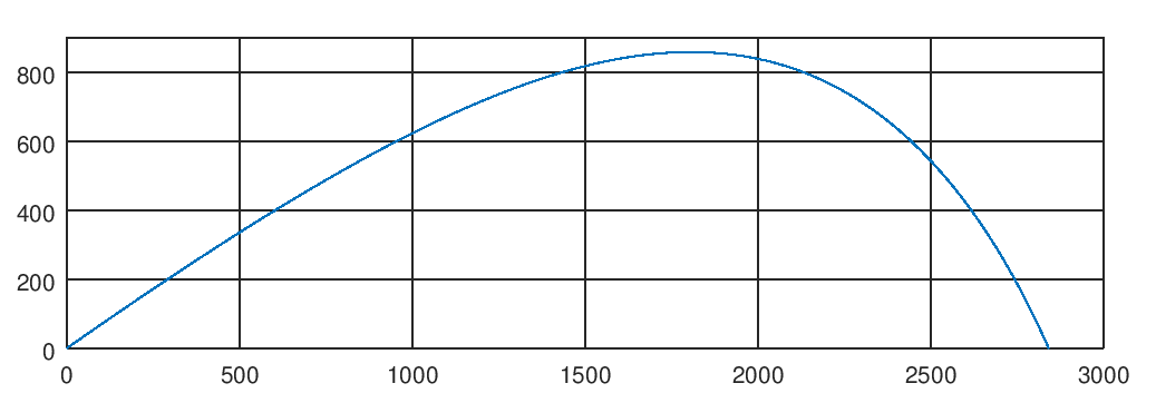
На выходе мы получили траекторию полета снаряда, что дает нам ориентировочные представления о характеристиках орудия: при заданных параметрах мы получили дальность стрельбы чуть более 2,5 км и высоту подъема снаряда чуть выше 800 метров. Точнее мы сказать не можем, вернее можем, если с карандашиком по сетке определим координаты нужных точек на графике. Но это, как известно, не наш метод. Хорошо бы получить эти данные с точностью, обеспечиваемой используемыми нами инструментами и без ручного труда. Вот об этом мы сегодня и поговорим.
1. Постановка задачи
Итак, построенная в прошлый раз математическая модель позволяет нам, для любого момента времени, определить координаты и скорость снаряда. По сути мы получили функции, которые позволяют вычислить следующие параметры траектории:

как функции времени. Высота полета снаряда это y(t). Если мы определим в какой момент времени высота становится равна нулю, то есть решим уравнение

относительно времени, то мы найдем момент времени
 в который снаряд упал на землю. Координата
 и будет дальность полета снаряда.
Как найти максимальную высоту подъема снаряда? Из графика траектории видно, что по мере подъема снаряда его траектория становится всё более и более пологой, пока в экстремальной точке скорость на мгновение становится горизонтальной и дальше снаряд движется вниз.
Говоря языком математики, необходимо найти точку экстремума функции
 . А что надо для этого сделать? Приравнять к нулю её производную! В данном случае производную по времени, то есть решить уравнение

или

ведь производная от вертикальной координаты по времени есть вертикальная проекция скорости. Корень этого уравнения,
 есть момент времени, когда снаряд достигнет максимальной высоты. Соответственно, интересующая нас высота

Просто? Более чем.
2. Уравнение, которого нет
И вот тут котенка Гава, как известно, ждут неприятности. Начнем с того, что даже если уравнение задано в виде формулы (аналитически) не всегда удается найти его решение. Вот например

Как вам? Простенько, но попробуйте найти икс, используя всё то, чему вас учили в школе. То-то же…
На самом деле ответ есть
Проведем некоторые эквивалентные преобразования

Введем замену
 , тогда
begin{align}
&u , e^{2 — u} = 1 \
&u , e^{-u} = e^{-2} \
&-u , e^{-u} = -e^{-2}
end{align}
Пусть теперь
 , тогда

Теперь делаем финт ушами. Математики прошлого хорошо поработали за нас. Если задана функция вида

то обратная ей функция, называется W-функцией Ламберта.

Не в даваясь в теорию ФКП, в которой я мало смыслю, скажу, что число
 попадает в интервал
 в котором функция Ламберта многозначна, значит корня будет два

откуда, раскручивая назад все замены получаем ответ

Приближенно этот ужас равен

Решение такого уравнения придется искать численно, тем более что очевидно его графическое решение
Графическое решение уравнения

В случае с моделью пушки всё несколько коварнее — наше уравнение задано даже не формулой. Оно задано, грубо говоря, таблицей значений фазовых координат, полученных для вполне конкретных параметров выстрела. У нас нет уравнения!
Ну так нам никто не мешает, чёрт возьми, это уравнение построить. Но, прежде чем начать писать скрипты, хочу извинится перед читателем, что ввёл его в заблуждение. В одном файле скрипта Octave можно размещать несколько функций, и имя файле на обязательно должно совпадать с именем функции. Достаточно, чтобы скрипт не начинался с определения функции.
Создадим новый скрипт в том же каталоге, где расположены файлы ballistics.m, f.m и f_air.m. Назовем его, например cannon.m. Для начала зададимся параметрами снаряда, начальной скоростью и направлением выстрела
%-------------------------------------------------------------------------------
% Параметры снаряда
%-------------------------------------------------------------------------------

% плотность материала снаряда
global gamma = 7800;
% коэффициент сопротивления формы (для шара)
global c_f = 0.47;
% калибр
global d = 0.1;

%-------------------------------------------------------------------------------
% Параметры стрельбы
%-------------------------------------------------------------------------------

% Начальная скорость
global v0 = 400;
% Угол наклона ствола пушки (в градусах!)
global alpha = 35;
А теперь напишем функцию, которая будет вычислять значения фазовых координат для произвольного момента времени
%-------------------------------------------------------------------------------
%   Расчет точки фазовой траектории для произвольного момента времени
%-------------------------------------------------------------------------------
function Y = MotionOdeSolve(v0, alpha, t)

  % Начальные условия
  x0 = 0;
  y0 = 0;
  vx0 = v0 * cos(deg2rad(alpha));
  vy0 = v0 * sin(deg2rad(alpha));

  Y0 = [x0; y0; vx0; vy0];

  % Решаем ОДУ движения
  solv = lsode("f_air", Y0, [0; t]);

  % Формируем вектор фазовых координат для момента времени t
  Y = [solv(2,1); solv(2,2); solv(2,3); solv(2,4)];

endfunction
Обратите внимание, теперь в качестве моментов времени, передаваемых функции решения уравнения мы берем всего два значения: начальный момент времени (t = 0) и интересующий нас момент времени. Соответственно, переменная solv будет содержать два вектора фазовых координат: начальный и тот который нам нужен. Собираем все компоненты конечной точки фазовой траектории в вектор Y и возвращаем его значение из функции.
Теперь нам ничего не стоит определить зависимость высоты полета снаряда от времени
%-------------------------------------------------------------------------------
% Вычисление высоты полета снаряда для произвольного момента времени
%-------------------------------------------------------------------------------
function h = height(t)

  global v0;
  global alpha;

  Y = MotionOdeSolve(v0, alpha, t);

  h = Y(2);

endfunction
протестируем полученную функцию
t1 = 10;
t2 = 20;
printf("h(%f) = %f, h(%f) = %fn", t1, height(t1), t2, height(t2));
При запуске скрипта на исполнение мы увидим в командном окне следующий вывод
>> cannon
h(10.000000) = 855.013452, h(20.000000) = 500.106649
Отлично, функция работает! Аналогично определим и функцию вычисления горизонтальной дальности
%-------------------------------------------------------------------------------
% Горизонтальное удаление снаряда от позиции стрельбы для произвольного t
%-------------------------------------------------------------------------------
function d = dist(t)

  global v0;
  global alpha;

  Y = MotionOdeSolve(v0, alpha, t);

  d = Y(1);

endfunction
Видно, что для вычисления высоты и дальности мы каждый раз интегрируем уравнения движения, от начального до интересующего нас момента времени. Таким образом мы получили зависимость, не выражаемую конкретной формулой. Это довольно круто.
3. Принципы численного решения нелинейных уравнений
Методы численного решения нелинейных и трансцендентных уравнений заточены под решение уравнений вида

К такой форме легко привести любое уравнение. Например
превращается в

где
 . Корни этого, эквивалентного уравнения, равны корням исходного. Если мы построим график функции f(x), то увидим такую картинку

корни уравнения это значения аргумента в тех точках, где график пересекает ось x.
Все методы численного решения таких уравнений включают в себя два этапа:
- Поиск начального приближения корня
- Уточнение корня с заданной погрешностью
Под начальным приближением понимают значение аргумента f(x), максимально близкое к корню, либо достаточно близкое, чтобы обеспечить сходимость метода за разумное количество итераций.
Простейшим методом является метод простых итераций. Для применения этого метода уравнение преобразуют к виду

и выполняю расчеты по рекуррентной формуле

В нашем примере

Посмотрим на график. У уравнения два корня. Найдем крайний левый корень, выбрав в качестве начального приближения


Ага, видно, что начиная с шестой итерации четвертый знак получающегося числа остается неизменным. Значит мы нашли корень уравнения с погрешностью менее 10-4 на шестой итерации.
Все бы хорошо, но метод простых итераций не всегда сходится. Попробуйте найти второй корень этого уравнения, задавшись любым, сколь угодно близким начальным приближением — у вас ничего не выйдет: каждое новое значение будет уходить от корня всё дальше и дальше. Сходимости метода можно добиться, существуют способы, но на практике это существенно осложняет нам жизнь. Поэтому для нахождения второго корня применим другой метод. Разложим исследуемую функцию в ряд Тейлора, в окрестности начального приближения

Ограничимся членами первого порядка малости, заменив саму функцию f(x) касательной к её графику в точке x0

и приравняв полученное выражение к нулю, решим его относительно x

Получаем итерационную формулу

В нашем примере

итерационная формула

В качестве начального приближения берем
 и пытаемся выполнять итерации

Как видно, этот метод сошелся за четыре итерации с точностью до четырех знаков. Этот метод называют методом Ньютона. Его достоинством является быстрая сходимость. Среди недостатков: высокая чувствительность к точности начального приближения и необходимость вычислять производную левой части уравнения. В случае, когда для уравнения нет аналитического выражения, приходится прибегать к мерзкой операции численного дифференцирования, что не всегда удобно и возможно.
Эти примеры я привел, чтобы объяснить общий принцип. Кроме этих двух методов существует ещё масса методов, например:
- Метод бисекции — отличается гарантированной сходимостью, однако с довольно низкой скоростью
- Метод хорд — не требует вычисления производной функции, обладает неплохой скоростью сходимости
Все перечисленные методы требуют предварительной подготовки, в виде поиска начального приближения или интервала изоляции корня — интервала изменения аргумента f(x), на границах которого функция меняет знак. В этом случае можно с уверенность сказать (при условии непрерывности функции!) что внутри интервала изоляции есть хотя бы один корень.
4. Определяем параметры траектории пушечного ядра
Итак, найдем момент времени, когда снаряд упадет на землю. Прежде всего, определим интервал изоляции корня
%
% Решаем задачу поиска дальности полета снаряда. Следует решить уравнение
%   height(t) = 0
% относительно времени.
%

% Поиск интервала изоляции корня
t0 = 0;
deltaT = 1.0;

t = t0;

while (height(t) >= 0)
  t = t + deltaT;
endwhile

b = t;
a = t - deltaT;

% Первое приближение корня
t1 = t - deltaT / 2;
Делаем это исходя из физического смысла задачи — после сразу выстрела высота полета снаряда неотрицательна. Перебираем все моменты времени, начиная от нуля, до тех пор, пока высота не станет отрицательна. Перебираем с достаточно крупным шагом (1 секунда) чтобы процедура не была слишком длительной, ведь на каждом шаге мы заново интегрируем дифференциальные уравнения движения, что весьма накладно сточки зрения вычислительных затрат. Как только высота станет отрицательной, заканчиваем перебор. Корень уравнения h(t) = 0 находится где-то внутри интервала [a, b]. Начальное приближение берем в середине этого интервала

Теперь отдаем уравнение на съедение процедуре решения нелинейных уравнений Octave
% Уточняем корень
t_end = fsolve("height", t1);
Функция fsolve() на вход принимает функцию, описывающую левую часть уравнения f(x) = 0 и значение начального приближения. Возвращает значение корня, вычисленное с заданной точностью. С какой точностью? Пока не будем задаваться этим вопросом и воспользуемся настройками по-умолчанию, на данном этапе они нас устраивают.
Получив значение момента времени падения, вычисляем дистанцию от позиции стрельбы
% Определяем дистанцию стрельбы
d_max = dist(t_end);
% выводим её в терминал
printf("Shot distance: %f, mn", d_max);
Аналогичным образом находим момент времени когда обнуляется вертикальная проекция скорости и вычисляем высоту полета снаряда в этот момент
%-------------------------------------------------------------------------------
% Вычисление вертикальной проекции вектора скорости
%-------------------------------------------------------------------------------
function v = vy(t)

  global v0;
  global alpha;

  Y = MotionOdeSolve(v0, alpha, t);

  v = Y(4);

endfunction

%
% Решаем задачу поиска максимальной высоты подъема снаряда. Следует решить
% уравнение
%
% vy(t) = 0
%

% Ищем интервал изоляции корня
t = t0;

while (vy(t) >= 0)
  t = t + deltaT;
endwhile

% Первое приближение корня
t1 = t - deltaT / 2;

% Уточняем корень
t_hmax = fsolve("vy", t1);

% Находим максимальную высоту подъема снаряда
h_max = height(t_hmax);

printf("Maximal height: %f, mn", h_max);
В командном окне можно увидеть результаты работы программы
>> cannon
h(10.000000) = 855.013452, h(20.000000) = 500.106649
Shot distance: 2840.991508, m
Maximal height: 857.963929, m
а также посмотреть, с какой точностью были решены уравнения
>> height(t_end)
ans =   -1.2328e-06
>> vy(t_hmax)
ans =    4.5117e-09
Для наших учебных целей точность вполне приемлема.
Заключение
Сегодня мы рассмотрели, несмотря опять таки на простоту примера, довольно широкий пласт задач. Теперь мы знаем, что отсутствие аналитических зависимостей, описывающих процесс, отнюдь не является препятствием к исследованию его характеристик. Нерешенной осталась задача определения максимальной дальности стрельбы, доступной для данной пушки, но об этот в другой раз. Спасибо за внимание!
поделиться знаниями или
запомнить страничку
- Все категории
-
экономические
43,662 -
гуманитарные
33,654 -
юридические
17,917 -
школьный раздел
611,978 -
разное
16,905
Популярное на сайте:
Как быстро выучить стихотворение наизусть? Запоминание стихов является стандартным заданием во многих школах.
Как научится читать по диагонали? Скорость чтения зависит от скорости восприятия каждого отдельного слова в тексте.
Как быстро и эффективно исправить почерк? Люди часто предполагают, что каллиграфия и почерк являются синонимами, но это не так.
Как научится говорить грамотно и правильно? Общение на хорошем, уверенном и естественном русском языке является достижимой целью.