In linear algebra, a rotation matrix is a transformation matrix that is used to perform a rotation in Euclidean space. For example, using the convention below, the matrix

rotates points in the xy plane counterclockwise through an angle θ about the origin of a two-dimensional Cartesian coordinate system. To perform the rotation on a plane point with standard coordinates v = (x, y), it should be written as a column vector, and multiplied by the matrix R:

If x and y are the endpoint coordinates of a vector, where x is cosine and y is sine, then the above equations become the trigonometric summation angle formulae. Indeed, a rotation matrix can be seen as the trigonometric summation angle formulae in matrix form. One way to understand this is say we have a vector at an angle 30° from the x axis, and we wish to rotate that angle by a further 45°. We simply need to compute the vector endpoint coordinates at 75°.
The examples in this article apply to active rotations of vectors counterclockwise in a right-handed coordinate system (y counterclockwise from x) by pre-multiplication (R on the left). If any one of these is changed (such as rotating axes instead of vectors, a passive transformation), then the inverse of the example matrix should be used, which coincides with its transpose.
Since matrix multiplication has no effect on the zero vector (the coordinates of the origin), rotation matrices describe rotations about the origin. Rotation matrices provide an algebraic description of such rotations, and are used extensively for computations in geometry, physics, and computer graphics. In some literature, the term rotation is generalized to include improper rotations, characterized by orthogonal matrices with a determinant of −1 (instead of +1). These combine proper rotations with reflections (which invert orientation). In other cases, where reflections are not being considered, the label proper may be dropped. The latter convention is followed in this article.
Rotation matrices are square matrices, with real entries. More specifically, they can be characterized as orthogonal matrices with determinant 1; that is, a square matrix R is a rotation matrix if and only if RT = R−1 and det R = 1. The set of all orthogonal matrices of size n with determinant +1 is a representation of a group known as the special orthogonal group SO(n), one example of which is the rotation group SO(3). The set of all orthogonal matrices of size n with determinant +1 or −1 is a representation of the (general) orthogonal group O(n).
In two dimensions[edit]

A counterclockwise rotation of a vector through angle θ. The vector is initially aligned with the x-axis.
In two dimensions, the standard rotation matrix has the following form:

This rotates column vectors by means of the following matrix multiplication,

Thus, the new coordinates (x′, y′) of a point (x, y) after rotation are

Examples[edit]
For example, when the vector
is rotated by an angle θ, its new coordinates are

and when the vector
is rotated by an angle θ, its new coordinates are

Direction[edit]
The direction of vector rotation is counterclockwise if θ is positive (e.g. 90°), and clockwise if θ is negative (e.g. −90°). Thus the clockwise rotation matrix is found as

The two-dimensional case is the only non-trivial (i.e. not one-dimensional) case where the rotation matrices group is commutative, so that it does not matter in which order multiple rotations are performed. An alternative convention uses rotating axes,[1] and the above matrices also represent a rotation of the axes clockwise through an angle θ.
Non-standard orientation of the coordinate system[edit]

A rotation through angle θ with non-standard axes.
If a standard right-handed Cartesian coordinate system is used, with the x-axis to the right and the y-axis up, the rotation R(θ) is counterclockwise. If a left-handed Cartesian coordinate system is used, with x directed to the right but y directed down, R(θ) is clockwise. Such non-standard orientations are rarely used in mathematics but are common in 2D computer graphics, which often have the origin in the top left corner and the y-axis down the screen or page.[2]
See below for other alternative conventions which may change the sense of the rotation produced by a rotation matrix.
Common rotations[edit]
Particularly useful are the matrices
![{displaystyle {begin{bmatrix}0&-1\[3pt]1&0\end{bmatrix}},quad {begin{bmatrix}-1&0\[3pt]0&-1\end{bmatrix}},quad {begin{bmatrix}0&1\[3pt]-1&0\end{bmatrix}}}](https://wikimedia.org/api/rest_v1/media/math/render/svg/049475f6bbfd9cfe4f0db0e7f063301e7acb774b)
for 90°, 180°, and 270° counter-clockwise rotations.
A 180° rotation (middle) followed by a positive 90° rotation (left) is equivalent to a single negative 90° (positive 270°) rotation (right). Each of these figures depicts the result of a rotation relative to an upright starting position (bottom left) and includes the matrix representation of the permutation applied by the rotation (center right), as well as other related diagrams. See «Permutation notation» on Wikiversity for details.
Relationship with complex plane[edit]
Since

the matrices of the shape

form a ring isomorphic to the field of the complex numbers  . Under this isomorphism, the rotation matrices correspond to circle of the unit complex numbers, the complex numbers of modulus 1.
If one identifies  with through the linear isomorphism
  the action of a matrix of the above form on vectors of corresponds to the multiplication by the complex number x + iy, and rotations correspond to multiplication by complex numbers of modulus 1.
As every rotation matrix can be written

the above correspondence associates such a matrix with the complex number

(this last equality is Euler’s formula).
In three dimensions[edit]
A positive 90° rotation around the y-axis (left) after one around the z-axis (middle) gives a 120° rotation around the main diagonal (right).
In the top left corner are the rotation matrices, in the bottom right corner are the corresponding permutations of the cube with the origin in its center.
Basic rotations[edit]
A basic rotation (also called elemental rotation) is a rotation about one of the axes of a coordinate system. The following three basic rotation matrices rotate vectors by an angle θ about the x-, y-, or z-axis, in three dimensions, using the right-hand rule—which codifies their alternating signs. Notice that the right-hand rule only works when multiplying  . (The same matrices can also represent a clockwise rotation of the axes.[nb 1])
![{displaystyle {begin{alignedat}{1}R_{x}(theta )&={begin{bmatrix}1&0&0\0&cos theta &-sin theta \[3pt]0&sin theta &cos theta \[3pt]end{bmatrix}}\[6pt]R_{y}(theta )&={begin{bmatrix}cos theta &0&sin theta \[3pt]0&1&0\[3pt]-sin theta &0&cos theta \end{bmatrix}}\[6pt]R_{z}(theta )&={begin{bmatrix}cos theta &-sin theta &0\[3pt]sin theta &cos theta &0\[3pt]0&0&1\end{bmatrix}}end{alignedat}}}](https://wikimedia.org/api/rest_v1/media/math/render/svg/a6821937d5031de282a190f75312353c970aa2df)
For column vectors, each of these basic vector rotations appears counterclockwise when the axis about which they occur points toward the observer, the coordinate system is right-handed, and the angle θ is positive. Rz, for instance, would rotate toward the y-axis a vector aligned with the x-axis, as can easily be checked by operating with Rz on the vector (1,0,0):

This is similar to the rotation produced by the above-mentioned two-dimensional rotation matrix. See below for alternative conventions which may apparently or actually invert the sense of the rotation produced by these matrices.
General rotations[edit]
Other rotation matrices can be obtained from these three using matrix multiplication. For example, the product

represents a rotation whose yaw, pitch, and roll angles are α, β and γ, respectively. More formally, it is an intrinsic rotation whose Tait–Bryan angles are α, β, γ, about axes z, y, x, respectively.
Similarly, the product

represents an extrinsic rotation whose (improper) Euler angles are α, β, γ, about axes x, y, z.
These matrices produce the desired effect only if they are used to premultiply column vectors, and (since in general matrix multiplication is not commutative) only if they are applied in the specified order (see Ambiguities for more details). The order of rotation operations is from right to left; the matrix adjacent to the column vector is the first to be applied, and then the one to the left.[3]
Conversion from rotation matrix to axis–angle[edit]
Every rotation in three dimensions is defined by its axis (a vector along this axis is unchanged by the rotation), and its angle — the amount of rotation about that axis (Euler rotation theorem).
There are several methods to compute the axis and angle from a rotation matrix (see also axis–angle representation). Here, we only describe the method based on the computation of the eigenvectors and eigenvalues of the rotation matrix. It is also possible to use the trace of the rotation matrix.
Determining the axis[edit]
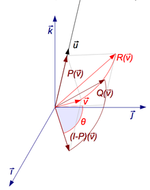
A rotation R around axis u can be decomposed using 3 endomorphisms P, (I − P), and Q (click to enlarge).
Given a 3 × 3 rotation matrix R, a vector u parallel to the rotation axis must satisfy

since the rotation of u around the rotation axis must result in u. The equation above may be solved for u which is unique up to a scalar factor unless R = I.
Further, the equation may be rewritten

which shows that u lies in the null space of R − I.
Viewed in another way, u is an eigenvector of R corresponding to the eigenvalue λ = 1. Every rotation matrix must have this eigenvalue, the other two eigenvalues being complex conjugates of each other. It follows that a general rotation matrix in three dimensions has, up to a multiplicative constant, only one real eigenvector.
One way to determine the rotation axis is by showing that:

Since (R − RT) is a skew-symmetric matrix, we can choose u such that
![{displaystyle [mathbf {u} ]_{times }=left(R-R^{mathsf {T}}right).}](https://wikimedia.org/api/rest_v1/media/math/render/svg/4f918d62cae11c81d33160177d9583d6e7efbe2d)
The matrix–vector product becomes a cross product of a vector with itself, ensuring that the result is zero:
![{displaystyle left(R-R^{mathsf {T}}right)mathbf {u} =[mathbf {u} ]_{times }mathbf {u} =mathbf {u} times mathbf {u} =0,}](https://wikimedia.org/api/rest_v1/media/math/render/svg/11848fee25bc229562a029195d181540a87e8597)
Therefore, if

then

The magnitude of u computed this way is ‖u‖ = 2 sin θ, where θ is the angle of rotation.
This does not work if R is symmetric. Above, if R − RT is zero, then all subsequent steps are invalid. In this case, it is necessary to diagonalize R and find the eigenvector corresponding to an eigenvalue of 1.
Determining the angle[edit]
To find the angle of a rotation, once the axis of the rotation is known, select a vector v perpendicular to the axis. Then the angle of the rotation is the angle between v and Rv.
A more direct method, however, is to simply calculate the trace: the sum of the diagonal elements of the rotation matrix. Care should be taken to select the right sign for the angle θ to match the chosen axis:

from which follows that the angle’s absolute value is

Rotation matrix from axis and angle[edit]
The matrix of a proper rotation R by angle θ around the axis u = (ux, uy, uz), a unit vector with u2
x + u2
y + u2
z = 1, is given by:[4]

A derivation of this matrix from first principles can be found in section 9.2 here.[5] The basic idea to derive this matrix is dividing the problem into few known simple steps.
- First rotate the given axis and the point such that the axis lies in one of the coordinate planes (xy, yz or zx)
- Then rotate the given axis and the point such that the axis is aligned with one of the two coordinate axes for that particular coordinate plane (x, y or z)
- Use one of the fundamental rotation matrices to rotate the point depending on the coordinate axis with which the rotation axis is aligned.
- Reverse rotate the axis-point pair such that it attains the final configuration as that was in step 2 (Undoing step 2)
- Reverse rotate the axis-point pair which was done in step 1 (undoing step 1)
This can be written more concisely as
![{displaystyle R=(cos theta ),I+(sin theta ),[mathbf {u} ]_{times }+(1-cos theta ),(mathbf {u} otimes mathbf {u} ),}](https://wikimedia.org/api/rest_v1/media/math/render/svg/5865faae48e2c8bca9a0780d52fec23a768e5354)
where [u]× is the cross product matrix of u; the expression u ⊗ u is the outer product, and I is the identity matrix. Alternatively, the matrix entries are:

where εjkl is the Levi-Civita symbol with ε123 = 1. This is a matrix form of Rodrigues’ rotation formula, (or the equivalent, differently parametrized Euler–Rodrigues formula) with[nb 2]
![{displaystyle mathbf {u} otimes mathbf {u} =mathbf {u} mathbf {u} ^{mathsf {T}}={begin{bmatrix}u_{x}^{2}&u_{x}u_{y}&u_{x}u_{z}\[3pt]u_{x}u_{y}&u_{y}^{2}&u_{y}u_{z}\[3pt]u_{x}u_{z}&u_{y}u_{z}&u_{z}^{2}end{bmatrix}},qquad [mathbf {u} ]_{times }={begin{bmatrix}0&-u_{z}&u_{y}\[3pt]u_{z}&0&-u_{x}\[3pt]-u_{y}&u_{x}&0end{bmatrix}}.}](https://wikimedia.org/api/rest_v1/media/math/render/svg/e3ddca93f49b042e6a14d5263002603fc0738308)
In  the rotation of a vector x around the axis u by an angle θ can be written as:

If the 3D space is right-handed and θ > 0, this rotation will be counterclockwise when u points towards the observer (Right-hand rule). Explicitly, with  a right-handed orthonormal basis,

Note the striking merely apparent differences to the equivalent Lie-algebraic formulation below.
Properties[edit]
For any n-dimensional rotation matrix R acting on 
 (The rotation is an orthogonal matrix)

It follows that:

A rotation is termed proper if det R = 1, and improper (or a roto-reflection) if det R = –1. For even dimensions n = 2k, the n eigenvalues λ of a proper rotation occur as pairs of complex conjugates which are roots of unity: λ = e±iθj for j = 1, …, k, which is real only for λ = ±1. Therefore, there may be no vectors fixed by the rotation (λ = 1), and thus no axis of rotation. Any fixed eigenvectors occur in pairs, and the axis of rotation is an even-dimensional subspace.
For odd dimensions n = 2k + 1, a proper rotation R will have an odd number of eigenvalues, with at least one λ = 1 and the axis of rotation will be an odd dimensional subspace. Proof:

Here I is the identity matrix, and we use det(RT) = det(R) = 1, as well as (−1)n = −1 since n is odd. Therefore, det(R – I) = 0, meaning there is a null vector v with (R – I)v = 0, that is Rv = v, a fixed eigenvector. There may also be pairs of fixed eigenvectors in the even-dimensional subspace orthogonal to v, so the total dimension of fixed eigenvectors is odd.
For example, in 2-space n = 2, a rotation by angle θ has eigenvalues λ = eiθ and λ = e−iθ, so there is no axis of rotation except when θ = 0, the case of the null rotation. In 3-space n = 3, the axis of a non-null proper rotation is always a unique line, and a rotation around this axis by angle θ has eigenvalues λ = 1, eiθ, e−iθ. In 4-space n = 4, the four eigenvalues are of the form e±iθ, e±iφ. The null rotation has θ = φ = 0. The case of θ = 0, φ ≠ 0 is called a simple rotation, with two unit eigenvalues forming an axis plane, and a two-dimensional rotation orthogonal to the axis plane. Otherwise, there is no axis plane. The case of θ = φ is called an isoclinic rotation, having eigenvalues e±iθ repeated twice, so every vector is rotated through an angle θ.
The trace of a rotation matrix is equal to the sum of its eigenvalues. For n = 2, a rotation by angle θ has trace 2 cos θ. For n = 3, a rotation around any axis by angle θ has trace 1 + 2 cos θ. For n = 4, and the trace is 2(cos θ + cos φ), which becomes 4 cos θ for an isoclinic rotation.
Examples[edit]
|
|


Geometry[edit]
In Euclidean geometry, a rotation is an example of an isometry, a transformation that moves points without changing the distances between them. Rotations are distinguished from other isometries by two additional properties: they leave (at least) one point fixed, and they leave «handedness» unchanged. In contrast, a translation moves every point, a reflection exchanges left- and right-handed ordering, a glide reflection does both, and an improper rotation combines a change in handedness with a normal rotation.
If a fixed point is taken as the origin of a Cartesian coordinate system, then every point can be given coordinates as a displacement from the origin. Thus one may work with the vector space of displacements instead of the points themselves. Now suppose (p1, …, pn) are the coordinates of the vector p from the origin O to point P. Choose an orthonormal basis for our coordinates; then the squared distance to P, by Pythagoras, is

which can be computed using the matrix multiplication

A geometric rotation transforms lines to lines, and preserves ratios of distances between points. From these properties it can be shown that a rotation is a linear transformation of the vectors, and thus can be written in matrix form, Qp. The fact that a rotation preserves, not just ratios, but distances themselves, is stated as

or

Because this equation holds for all vectors, p, one concludes that every rotation matrix, Q, satisfies the orthogonality condition,

Rotations preserve handedness because they cannot change the ordering of the axes, which implies the special matrix condition,

Equally important, it can be shown that any matrix satisfying these two conditions acts as a rotation.
Multiplication[edit]
The inverse of a rotation matrix is its transpose, which is also a rotation matrix:

The product of two rotation matrices is a rotation matrix:

For n > 2, multiplication of n × n rotation matrices is generally not commutative.

Noting that any identity matrix is a rotation matrix, and that matrix multiplication is associative, we may summarize all these properties by saying that the n × n rotation matrices form a group, which for n > 2 is non-abelian, called a special orthogonal group, and denoted by SO(n), SO(n,R), SOn, or SOn(R), the group of n × n rotation matrices is isomorphic to the group of rotations in an n-dimensional space. This means that multiplication of rotation matrices corresponds to composition of rotations, applied in left-to-right order of their corresponding matrices.
Ambiguities[edit]

Alias and alibi rotations
The interpretation of a rotation matrix can be subject to many ambiguities.
In most cases the effect of the ambiguity is equivalent to the effect of a rotation matrix inversion (for these orthogonal matrices equivalently matrix transpose).
- Alias or alibi (passive or active) transformation
- The coordinates of a point P may change due to either a rotation of the coordinate system CS (alias), or a rotation of the point P (alibi). In the latter case, the rotation of P also produces a rotation of the vector v representing P. In other words, either P and v are fixed while CS rotates (alias), or CS is fixed while P and v rotate (alibi). Any given rotation can be legitimately described both ways, as vectors and coordinate systems actually rotate with respect to each other, about the same axis but in opposite directions. Throughout this article, we chose the alibi approach to describe rotations. For instance,
- represents a counterclockwise rotation of a vector v by an angle θ, or a rotation of CS by the same angle but in the opposite direction (i.e. clockwise). Alibi and alias transformations are also known as active and passive transformations, respectively.
- Pre-multiplication or post-multiplication
- The same point P can be represented either by a column vector v or a row vector w. Rotation matrices can either pre-multiply column vectors (Rv), or post-multiply row vectors (wR). However, Rv produces a rotation in the opposite direction with respect to wR. Throughout this article, rotations produced on column vectors are described by means of a pre-multiplication. To obtain exactly the same rotation (i.e. the same final coordinates of point P), the equivalent row vector must be post-multiplied by the transpose of R (i.e. wRT).
- Right- or left-handed coordinates
- The matrix and the vector can be represented with respect to a right-handed or left-handed coordinate system. Throughout the article, we assumed a right-handed orientation, unless otherwise specified.
- Vectors or forms
- The vector space has a dual space of linear forms, and the matrix can act on either vectors or forms.

Decompositions[edit]
Independent planes[edit]
Consider the 3 × 3 rotation matrix

If Q acts in a certain direction, v, purely as a scaling by a factor λ, then we have

so that

Thus λ is a root of the characteristic polynomial for Q,

Two features are noteworthy. First, one of the roots (or eigenvalues) is 1, which tells us that some direction is unaffected by the matrix. For rotations in three dimensions, this is the axis of the rotation (a concept that has no meaning in any other dimension). Second, the other two roots are a pair of complex conjugates, whose product is 1 (the constant term of the quadratic), and whose sum is 2 cos θ (the negated linear term). This factorization is of interest for 3 × 3 rotation matrices because the same thing occurs for all of them. (As special cases, for a null rotation the «complex conjugates» are both 1, and for a 180° rotation they are both −1.) Furthermore, a similar factorization holds for any n × n rotation matrix. If the dimension, n, is odd, there will be a «dangling» eigenvalue of 1; and for any dimension the rest of the polynomial factors into quadratic terms like the one here (with the two special cases noted). We are guaranteed that the characteristic polynomial will have degree n and thus n eigenvalues. And since a rotation matrix commutes with its transpose, it is a normal matrix, so can be diagonalized. We conclude that every rotation matrix, when expressed in a suitable coordinate system, partitions into independent rotations of two-dimensional subspaces, at most n/2 of them.
The sum of the entries on the main diagonal of a matrix is called the trace; it does not change if we reorient the coordinate system, and always equals the sum of the eigenvalues. This has the convenient implication for 2 × 2 and 3 × 3 rotation matrices that the trace reveals the angle of rotation, θ, in the two-dimensional space (or subspace). For a 2 × 2 matrix the trace is 2 cos θ, and for a 3 × 3 matrix it is 1 + 2 cos θ. In the three-dimensional case, the subspace consists of all vectors perpendicular to the rotation axis (the invariant direction, with eigenvalue 1). Thus we can extract from any 3 × 3 rotation matrix a rotation axis and an angle, and these completely determine the rotation.
Sequential angles[edit]
The constraints on a 2 × 2 rotation matrix imply that it must have the form

with a2 + b2 = 1. Therefore, we may set a = cos θ and b = sin θ, for some angle θ. To solve for θ it is not enough to look at a alone or b alone; we must consider both together to place the angle in the correct quadrant, using a two-argument arctangent function.
Now consider the first column of a 3 × 3 rotation matrix,

Although a2 + b2 will probably not equal 1, but some value r2 < 1, we can use a slight variation of the previous computation to find a so-called Givens rotation that transforms the column to

zeroing b. This acts on the subspace spanned by the x— and y-axes. We can then repeat the process for the xz-subspace to zero c. Acting on the full matrix, these two rotations produce the schematic form

Shifting attention to the second column, a Givens rotation of the yz-subspace can now zero the z value. This brings the full matrix to the form

which is an identity matrix. Thus we have decomposed Q as

An n × n rotation matrix will have (n − 1) + (n − 2) + ⋯ + 2 + 1, or

entries below the diagonal to zero. We can zero them by extending the same idea of stepping through the columns with a series of rotations in a fixed sequence of planes. We conclude that the set of n × n rotation matrices, each of which has n2 entries, can be parameterized by 1/2n(n − 1) angles.
| xzxw | xzyw | xyxw | xyzw |
| yxyw | yxzw | yzyw | yzxw |
| zyzw | zyxw | zxzw | zxyw |
| xzxb | yzxb | xyxb | zyxb |
| yxyb | zxyb | yzyb | xzyb |
| zyzb | xyzb | zxzb | yxzb |
In three dimensions this restates in matrix form an observation made by Euler, so mathematicians call the ordered sequence of three angles Euler angles. However, the situation is somewhat more complicated than we have so far indicated. Despite the small dimension, we actually have considerable freedom in the sequence of axis pairs we use; and we also have some freedom in the choice of angles. Thus we find many different conventions employed when three-dimensional rotations are parameterized for physics, or medicine, or chemistry, or other disciplines. When we include the option of world axes or body axes, 24 different sequences are possible. And while some disciplines call any sequence Euler angles, others give different names (Cardano, Tait–Bryan, roll-pitch-yaw) to different sequences.
One reason for the large number of options is that, as noted previously, rotations in three dimensions (and higher) do not commute. If we reverse a given sequence of rotations, we get a different outcome. This also implies that we cannot compose two rotations by adding their corresponding angles. Thus Euler angles are not vectors, despite a similarity in appearance as a triplet of numbers.
Nested dimensions[edit]
A 3 × 3 rotation matrix such as

suggests a 2 × 2 rotation matrix,

is embedded in the upper left corner:
![{displaystyle Q_{3times 3}=left[{begin{matrix}Q_{2times 2}&mathbf {0} \mathbf {0} ^{mathsf {T}}&1end{matrix}}right].}](https://wikimedia.org/api/rest_v1/media/math/render/svg/6f439ce8b73f47040b70c9b64ab7fa89d91c46a6)
This is no illusion; not just one, but many, copies of n-dimensional rotations are found within (n + 1)-dimensional rotations, as subgroups. Each embedding leaves one direction fixed, which in the case of 3 × 3 matrices is the rotation axis. For example, we have
![{displaystyle {begin{aligned}Q_{mathbf {x} }(theta )&={begin{bmatrix}{color {CadetBlue}1}&{color {CadetBlue}0}&{color {CadetBlue}0}\{color {CadetBlue}0}&cos theta &-sin theta \{color {CadetBlue}0}&sin theta &cos theta end{bmatrix}},\[8px]Q_{mathbf {y} }(theta )&={begin{bmatrix}cos theta &{color {CadetBlue}0}&sin theta \{color {CadetBlue}0}&{color {CadetBlue}1}&{color {CadetBlue}0}\-sin theta &{color {CadetBlue}0}&cos theta end{bmatrix}},\[8px]Q_{mathbf {z} }(theta )&={begin{bmatrix}cos theta &-sin theta &{color {CadetBlue}0}\sin theta &cos theta &{color {CadetBlue}0}\{color {CadetBlue}0}&{color {CadetBlue}0}&{color {CadetBlue}1}end{bmatrix}},end{aligned}}}](https://wikimedia.org/api/rest_v1/media/math/render/svg/63ce9d4e595deed5ef5572d36ec99821e1b021e2)
fixing the x-axis, the y-axis, and the z-axis, respectively. The rotation axis need not be a coordinate axis; if u = (x,y,z) is a unit vector in the desired direction, then
![{displaystyle {begin{aligned}Q_{mathbf {u} }(theta )&={begin{bmatrix}0&-z&y\z&0&-x\-y&x&0end{bmatrix}}sin theta +left(I-mathbf {u} mathbf {u} ^{mathsf {T}}right)cos theta +mathbf {u} mathbf {u} ^{mathsf {T}}\[8px]&={begin{bmatrix}left(1-x^{2}right)c_{theta }+x^{2}&-zs_{theta }-xyc_{theta }+xy&ys_{theta }-xzc_{theta }+xz\zs_{theta }-xyc_{theta }+xy&left(1-y^{2}right)c_{theta }+y^{2}&-xs_{theta }-yzc_{theta }+yz\-ys_{theta }-xzc_{theta }+xz&xs_{theta }-yzc_{theta }+yz&left(1-z^{2}right)c_{theta }+z^{2}end{bmatrix}}\[8px]&={begin{bmatrix}x^{2}(1-c_{theta })+c_{theta }&xy(1-c_{theta })-zs_{theta }&xz(1-c_{theta })+ys_{theta }\xy(1-c_{theta })+zs_{theta }&y^{2}(1-c_{theta })+c_{theta }&yz(1-c_{theta })-xs_{theta }\xz(1-c_{theta })-ys_{theta }&yz(1-c_{theta })+xs_{theta }&z^{2}(1-c_{theta })+c_{theta }end{bmatrix}},end{aligned}}}](https://wikimedia.org/api/rest_v1/media/math/render/svg/87042389f5f93fc21a43beafc126d3ea5a9ee177)
where cθ = cos θ, sθ = sin θ, is a rotation by angle θ leaving axis u fixed.
A direction in (n + 1)-dimensional space will be a unit magnitude vector, which we may consider a point on a generalized sphere, Sn. Thus it is natural to describe the rotation group SO(n + 1) as combining SO(n) and Sn. A suitable formalism is the fiber bundle,

where for every direction in the base space, Sn, the fiber over it in the total space, SO(n + 1), is a copy of the fiber space, SO(n), namely the rotations that keep that direction fixed.
Thus we can build an n × n rotation matrix by starting with a 2 × 2 matrix, aiming its fixed axis on S2 (the ordinary sphere in three-dimensional space), aiming the resulting rotation on S3, and so on up through Sn−1. A point on Sn can be selected using n numbers, so we again have 1/2n(n − 1) numbers to describe any n × n rotation matrix.
In fact, we can view the sequential angle decomposition, discussed previously, as reversing this process. The composition of n − 1 Givens rotations brings the first column (and row) to (1, 0, …, 0), so that the remainder of the matrix is a rotation matrix of dimension one less, embedded so as to leave (1, 0, …, 0) fixed.
Skew parameters via Cayley’s formula[edit]
When an n × n rotation matrix Q, does not include a −1 eigenvalue, thus none of the planar rotations which it comprises are 180° rotations, then Q + I is an invertible matrix. Most rotation matrices fit this description, and for them it can be shown that (Q − I)(Q + I)−1 is a skew-symmetric matrix, A. Thus AT = −A; and since the diagonal is necessarily zero, and since the upper triangle determines the lower one, A contains 1/2n(n − 1) independent numbers.
Conveniently, I − A is invertible whenever A is skew-symmetric; thus we can recover the original matrix using the Cayley transform,

which maps any skew-symmetric matrix A to a rotation matrix. In fact, aside from the noted exceptions, we can produce any rotation matrix in this way. Although in practical applications we can hardly afford to ignore 180° rotations, the Cayley transform is still a potentially useful tool, giving a parameterization of most rotation matrices without trigonometric functions.
In three dimensions, for example, we have (Cayley 1846)
![{displaystyle {begin{aligned}&{begin{bmatrix}0&-z&y\z&0&-x\-y&x&0end{bmatrix}}mapsto \[3pt]quad {frac {1}{1+x^{2}+y^{2}+z^{2}}}&{begin{bmatrix}1+x^{2}-y^{2}-z^{2}&2xy-2z&2y+2xz\2xy+2z&1-x^{2}+y^{2}-z^{2}&2yz-2x\2xz-2y&2x+2yz&1-x^{2}-y^{2}+z^{2}end{bmatrix}}.end{aligned}}}](https://wikimedia.org/api/rest_v1/media/math/render/svg/ad82b169b68ec60349be493378761aab543c9cf8)
If we condense the skew entries into a vector, (x,y,z), then we produce a 90° rotation around the x-axis for (1, 0, 0), around the y-axis for (0, 1, 0), and around the z-axis for (0, 0, 1). The 180° rotations are just out of reach; for, in the limit as x → ∞, (x, 0, 0) does approach a 180° rotation around the x axis, and similarly for other directions.
Decomposition into shears[edit]
For the 2D case, a rotation matrix can be decomposed into three shear matrices (Paeth 1986):

This is useful, for instance, in computer graphics, since shears can be implemented with fewer multiplication instructions than rotating a bitmap directly. On modern computers, this may not matter, but it can be relevant for very old or low-end microprocessors.
A rotation can also be written as two shears and scaling (Daubechies & Sweldens 1998):

Group theory[edit]
Below follow some basic facts about the role of the collection of all rotation matrices of a fixed dimension (here mostly 3) in mathematics and particularly in physics where rotational symmetry is a requirement of every truly fundamental law (due to the assumption of isotropy of space), and where the same symmetry, when present, is a simplifying property of many problems of less fundamental nature. Examples abound in classical mechanics and quantum mechanics. Knowledge of the part of the solutions pertaining to this symmetry applies (with qualifications) to all such problems and it can be factored out of a specific problem at hand, thus reducing its complexity. A prime example – in mathematics and physics – would be the theory of spherical harmonics. Their role in the group theory of the rotation groups is that of being a representation space for the entire set of finite-dimensional irreducible representations of the rotation group SO(3). For this topic, see Rotation group SO(3) § Spherical harmonics.
The main articles listed in each subsection are referred to for more detail.
Lie group[edit]
The n × n rotation matrices for each n form a group, the special orthogonal group, SO(n). This algebraic structure is coupled with a topological structure inherited from  in such a way that the operations of multiplication and taking the inverse are analytic functions of the matrix entries. Thus SO(n) is for each n a Lie group. It is compact and connected, but not simply connected. It is also a semi-simple group, in fact a simple group with the exception SO(4).[6] The relevance of this is that all theorems and all machinery from the theory of analytic manifolds (analytic manifolds are in particular smooth manifolds) apply and the well-developed representation theory of compact semi-simple groups is ready for use.
Lie algebra[edit]
The Lie algebra so(n) of SO(n) is given by

and is the space of skew-symmetric matrices of dimension n, see classical group, where o(n) is the Lie algebra of O(n), the orthogonal group. For reference, the most common basis for so(3) is

Exponential map[edit]
Connecting the Lie algebra to the Lie group is the exponential map, which is defined using the standard matrix exponential series for eA[7] For any skew-symmetric matrix A, exp(A) is always a rotation matrix.[nb 3]
An important practical example is the 3 × 3 case. In rotation group SO(3), it is shown that one can identify every A ∈ so(3) with an Euler vector ω = θu, where u = (x, y, z) is a unit magnitude vector.
By the properties of the identification  , u is in the null space of A. Thus, u is left invariant by exp(A) and is hence a rotation axis.
According to Rodrigues’ rotation formula on matrix form, one obtains,

where

This is the matrix for a rotation around axis u by the angle θ. For full detail, see exponential map SO(3).
Baker–Campbell–Hausdorff formula[edit]
The BCH formula provides an explicit expression for Z = log(eXeY) in terms of a series expansion of nested commutators of X and Y.[8] This general expansion unfolds as[nb 4]
![{displaystyle Z=C(X,Y)=X+Y+{tfrac {1}{2}}[X,Y]+{tfrac {1}{12}}{bigl [}X,[X,Y]{bigr ]}-{tfrac {1}{12}}{bigl [}Y,[X,Y]{bigr ]}+cdots .}](https://wikimedia.org/api/rest_v1/media/math/render/svg/18d3139eecb4a3799df3f187e78c1b3f0cb2f3bf)
In the 3 × 3 case, the general infinite expansion has a compact form,[9]
![Z=alpha X+beta Y+gamma [X,Y],](https://wikimedia.org/api/rest_v1/media/math/render/svg/1cdd2c4da063f9ec30359beaacd3767b962f3875)
for suitable trigonometric function coefficients, detailed in the Baker–Campbell–Hausdorff formula for SO(3).
As a group identity, the above holds for all faithful representations, including the doublet (spinor representation), which is simpler. The same explicit formula thus follows straightforwardly through Pauli matrices; see the 2 × 2 derivation for SU(2). For the general n × n case, one might use Ref.[10]
Spin group[edit]
The Lie group of n × n rotation matrices, SO(n), is not simply connected, so Lie theory tells us it is a homomorphic image of a universal covering group. Often the covering group, which in this case is called the spin group denoted by Spin(n), is simpler and more natural to work with.[11]
In the case of planar rotations, SO(2) is topologically a circle, S1. Its universal covering group, Spin(2), is isomorphic to the real line, R, under addition. Whenever angles of arbitrary magnitude are used one is taking advantage of the convenience of the universal cover. Every 2 × 2 rotation matrix is produced by a countable infinity of angles, separated by integer multiples of 2π. Correspondingly, the fundamental group of SO(2) is isomorphic to the integers, Z.
In the case of spatial rotations, SO(3) is topologically equivalent to three-dimensional real projective space, RP3. Its universal covering group, Spin(3), is isomorphic to the 3-sphere, S3. Every 3 × 3 rotation matrix is produced by two opposite points on the sphere. Correspondingly, the fundamental group of SO(3) is isomorphic to the two-element group, Z2.
We can also describe Spin(3) as isomorphic to quaternions of unit norm under multiplication, or to certain 4 × 4 real matrices, or to 2 × 2 complex special unitary matrices, namely SU(2). The covering maps for the first and the last case are given by

and

For a detailed account of the SU(2)-covering and the quaternionic covering, see spin group SO(3).
Many features of these cases are the same for higher dimensions. The coverings are all two-to-one, with SO(n), n > 2, having fundamental group Z2. The natural setting for these groups is within a Clifford algebra. One type of action of the rotations is produced by a kind of «sandwich», denoted by qvq∗. More importantly in applications to physics, the corresponding spin representation of the Lie algebra sits inside the Clifford algebra. It can be exponentiated in the usual way to give rise to a 2-valued representation, also known as projective representation of the rotation group. This is the case with SO(3) and SU(2), where the 2-valued representation can be viewed as an «inverse» of the covering map. By properties of covering maps, the inverse can be chosen ono-to-one as a local section, but not globally.
Infinitesimal rotations[edit]
The matrices in the Lie algebra are not themselves rotations; the skew-symmetric matrices are derivatives, proportional differences of rotations. An actual «differential rotation», or infinitesimal rotation matrix has the form

where dθ is vanishingly small and A ∈ so(n), for instance with A = Lx,

The computation rules are as usual except that infinitesimals of second order are routinely dropped. With these rules, these matrices do not satisfy all the same properties as ordinary finite rotation matrices under the usual treatment of infinitesimals.[12] It turns out that the order in which infinitesimal rotations are applied is irrelevant. To see this exemplified, consult infinitesimal rotations SO(3).
Conversions[edit]
We have seen the existence of several decompositions that apply in any dimension, namely independent planes, sequential angles, and nested dimensions. In all these cases we can either decompose a matrix or construct one. We have also given special attention to 3 × 3 rotation matrices, and these warrant further attention, in both directions (Stuelpnagel 1964).
Quaternion[edit]
Given the unit quaternion q = w + xi + yj + zk, the equivalent pre-multiplied (to be used with column vectors) 3 × 3 rotation matrix is [13]

Now every quaternion component appears multiplied by two in a term of degree two, and if all such terms are zero what is left is an identity matrix. This leads to an efficient, robust conversion from any quaternion – whether unit or non-unit – to a 3 × 3 rotation matrix. Given:

we can calculate

Freed from the demand for a unit quaternion, we find that nonzero quaternions act as homogeneous coordinates for 3 × 3 rotation matrices. The Cayley transform, discussed earlier, is obtained by scaling the quaternion so that its w component is 1. For a 180° rotation around any axis, w will be zero, which explains the Cayley limitation.
The sum of the entries along the main diagonal (the trace), plus one, equals 4 − 4(x2 + y2 + z2), which is 4w2. Thus we can write the trace itself as 2w2 + 2w2 − 1; and from the previous version of the matrix we see that the diagonal entries themselves have the same form: 2x2 + 2w2 − 1, 2y2 + 2w2 − 1, and 2z2 + 2w2 − 1. So we can easily compare the magnitudes of all four quaternion components using the matrix diagonal. We can, in fact, obtain all four magnitudes using sums and square roots, and choose consistent signs using the skew-symmetric part of the off-diagonal entries:

Alternatively, use a single square root and division

This is numerically stable so long as the trace, t, is not negative; otherwise, we risk dividing by (nearly) zero. In that case, suppose Qxx is the largest diagonal entry, so x will have the largest magnitude (the other cases are derived by cyclic permutation); then the following is safe.

If the matrix contains significant error, such as accumulated numerical error, we may construct a symmetric 4 × 4 matrix,

and find the eigenvector, (x, y, z, w), of its largest magnitude eigenvalue. (If Q is truly a rotation matrix, that value will be 1.) The quaternion so obtained will correspond to the rotation matrix closest to the given matrix (Bar-Itzhack 2000) (Note: formulation of the cited article is post-multiplied, works with row vectors).
Polar decomposition[edit]
If the n × n matrix M is nonsingular, its columns are linearly independent vectors; thus the Gram–Schmidt process can adjust them to be an orthonormal basis. Stated in terms of numerical linear algebra, we convert M to an orthogonal matrix, Q, using QR decomposition. However, we often prefer a Q closest to M, which this method does not accomplish. For that, the tool we want is the polar decomposition (Fan & Hoffman 1955; Higham 1989).
To measure closeness, we may use any matrix norm invariant under orthogonal transformations. A convenient choice is the Frobenius norm, ‖Q − M‖F, squared, which is the sum of the squares of the element differences. Writing this in terms of the trace, Tr, our goal is,
- Find Q minimizing Tr( (Q − M)T(Q − M) ), subject to QTQ = I.
Though written in matrix terms, the objective function is just a quadratic polynomial. We can minimize it in the usual way, by finding where its derivative is zero. For a 3 × 3 matrix, the orthogonality constraint implies six scalar equalities that the entries of Q must satisfy. To incorporate the constraint(s), we may employ a standard technique, Lagrange multipliers, assembled as a symmetric matrix, Y. Thus our method is:
- Differentiate Tr( (Q − M)T(Q − M) + (QTQ − I)Y ) with respect to (the entries of) Q, and equate to zero.
Consider a 2 × 2 example. Including constraints, we seek to minimize

Taking the derivative with respect to Qxx, Qxy, Qyx, Qyy in turn, we assemble a matrix.

In general, we obtain the equation

so that

where Q is orthogonal and S is symmetric. To ensure a minimum, the Y matrix (and hence S) must be positive definite. Linear algebra calls QS the polar decomposition of M, with S the positive square root of S2 = MTM.

When M is non-singular, the Q and S factors of the polar decomposition are uniquely determined. However, the determinant of S is positive because S is positive definite, so Q inherits the sign of the determinant of M. That is, Q is only guaranteed to be orthogonal, not a rotation matrix. This is unavoidable; an M with negative determinant has no uniquely defined closest rotation matrix.
Axis and angle[edit]
To efficiently construct a rotation matrix Q from an angle θ and a unit axis u, we can take advantage of symmetry and skew-symmetry within the entries. If x, y, and z are the components of the unit vector representing the axis, and

then

Determining an axis and angle, like determining a quaternion, is only possible up to the sign; that is, (u, θ) and (−u, −θ) correspond to the same rotation matrix, just like q and −q. Additionally, axis–angle extraction presents additional difficulties. The angle can be restricted to be from 0° to 180°, but angles are formally ambiguous by multiples of 360°. When the angle is zero, the axis is undefined. When the angle is 180°, the matrix becomes symmetric, which has implications in extracting the axis. Near multiples of 180°, care is needed to avoid numerical problems: in extracting the angle, a two-argument arctangent with atan2(sin θ, cos θ) equal to θ avoids the insensitivity of arccos; and in computing the axis magnitude in order to force unit magnitude, a brute-force approach can lose accuracy through underflow (Moler & Morrison 1983).
A partial approach is as follows:

The x-, y-, and z-components of the axis would then be divided by r. A fully robust approach will use a different algorithm when t, the trace of the matrix Q, is negative, as with quaternion extraction. When r is zero because the angle is zero, an axis must be provided from some source other than the matrix.
Euler angles[edit]
Complexity of conversion escalates with Euler angles (used here in the broad sense). The first difficulty is to establish which of the twenty-four variations of Cartesian axis order we will use. Suppose the three angles are θ1, θ2, θ3; physics and chemistry may interpret these as

while aircraft dynamics may use

One systematic approach begins with choosing the rightmost axis. Among all permutations of (x,y,z), only two place that axis first; one is an even permutation and the other odd. Choosing parity thus establishes the middle axis. That leaves two choices for the left-most axis, either duplicating the first or not. These three choices gives us 3 × 2 × 2 = 12 variations; we double that to 24 by choosing static or rotating axes.
This is enough to construct a matrix from angles, but triples differing in many ways can give the same rotation matrix. For example, suppose we use the zyz convention above; then we have the following equivalent pairs:
-
(90°, 45°, −105°) ≡ (−270°, −315°, 255°) multiples of 360° (72°, 0°, 0°) ≡ (40°, 0°, 32°) singular alignment (45°, 60°, −30°) ≡ (−135°, −60°, 150°) bistable flip
Angles for any order can be found using a concise common routine (Herter & Lott 1993; Shoemake 1994).
The problem of singular alignment, the mathematical analog of physical gimbal lock, occurs when the middle rotation aligns the axes of the first and last rotations. It afflicts every axis order at either even or odd multiples of 90°. These singularities are not characteristic of the rotation matrix as such, and only occur with the usage of Euler angles.
The singularities are avoided when considering and manipulating the rotation matrix as orthonormal row vectors (in 3D applications often named the right-vector, up-vector and out-vector) instead of as angles. The singularities are also avoided when working with quaternions.
Vector to vector formulation[edit]
In some instances it is interesting to describe a rotation by specifying how a vector is mapped into another through the shortest path (smallest angle). In this completely describes the associated rotation matrix. In general, given x, y ∈  n, the matrix

belongs to SO(n + 1) and maps x to y.[14]
Uniform random rotation matrices[edit]
We sometimes need to generate a uniformly distributed random rotation matrix. It seems intuitively clear in two dimensions that this means the rotation angle is uniformly distributed between 0 and 2π. That intuition is correct, but does not carry over to higher dimensions. For example, if we decompose 3 × 3 rotation matrices in axis–angle form, the angle should not be uniformly distributed; the probability that (the magnitude of) the angle is at most θ should be 1/π(θ − sin θ), for 0 ≤ θ ≤ π.
Since SO(n) is a connected and locally compact Lie group, we have a simple standard criterion for uniformity, namely that the distribution be unchanged when composed with any arbitrary rotation (a Lie group «translation»). This definition corresponds to what is called Haar measure. León, Massé & Rivest (2006) show how to use the Cayley transform to generate and test matrices according to this criterion.
We can also generate a uniform distribution in any dimension using the subgroup algorithm of Diaconis & Shashahani (1987). This recursively exploits the nested dimensions group structure of SO(n), as follows. Generate a uniform angle and construct a 2 × 2 rotation matrix. To step from n to n + 1, generate a vector v uniformly distributed on the n-sphere Sn, embed the n × n matrix in the next larger size with last column (0, …, 0, 1), and rotate the larger matrix so the last column becomes v.
As usual, we have special alternatives for the 3 × 3 case. Each of these methods begins with three independent random scalars uniformly distributed on the unit interval. Arvo (1992) takes advantage of the odd dimension to change a Householder reflection to a rotation by negation, and uses that to aim the axis of a uniform planar rotation.
Another method uses unit quaternions. Multiplication of rotation matrices is homomorphic to multiplication of quaternions, and multiplication by a unit quaternion rotates the unit sphere. Since the homomorphism is a local isometry, we immediately conclude that to produce a uniform distribution on SO(3) we may use a uniform distribution on S3. In practice: create a four-element vector where each element is a sampling of a normal distribution. Normalize its length and you have a uniformly sampled random unit quaternion which represents a uniformly sampled random rotation. Note that the aforementioned only applies to rotations in dimension 3. For a generalised idea of quaternions, one should look into Rotors.
Euler angles can also be used, though not with each angle uniformly distributed (Murnaghan 1962; Miles 1965).
For the axis–angle form, the axis is uniformly distributed over the unit sphere of directions, S2, while the angle has the nonuniform distribution over [0,π] noted previously (Miles 1965).
See also[edit]
- Euler–Rodrigues formula
- Euler’s rotation theorem
- Rodrigues’ rotation formula
- Plane of rotation
- Axis–angle representation
- Rotation group SO(3)
- Rotation formalisms in three dimensions
- Rotation operator (vector space)
- Transformation matrix
- Yaw-pitch-roll system
- Kabsch algorithm
- Isometry
- Rigid transformation
- Rotations in 4-dimensional Euclidean space
- Trigonometric Identities
- Versor
[edit]
- ^ Note that if instead of rotating vectors, it is the reference frame that is being rotated, the signs on the sin θ terms will be reversed. If reference frame A is rotated anti-clockwise about the origin through an angle θ to create reference frame B, then Rx (with the signs flipped) will transform a vector described in reference frame A coordinates to reference frame B coordinates. Coordinate frame transformations in aerospace, robotics, and other fields are often performed using this interpretation of the rotation matrix.
- ^ Note that
so that, in Rodrigues’ notation, equivalently,
- ^ Note that this exponential map of skew-symmetric matrices to rotation matrices is quite different from the Cayley transform discussed earlier, differing to the third order,
Conversely, a skew-symmetric matrix A specifying a rotation matrix through the Cayley map specifies the same rotation matrix through the map exp(2 artanh A).
- ^ For a detailed derivation, see Derivative of the exponential map. Issues of convergence of this series to the right element of the Lie algebra are here swept under the carpet. Convergence is guaranteed when ‖X‖ + ‖Y‖ < log 2 and ‖Z‖ < log 2. If these conditions are not fulfilled, the series may still converge. A solution always exists since exp is onto[clarification needed] in the cases under consideration.
![{displaystyle mathbf {u} otimes mathbf {u} ={bigl (}[mathbf {u} ]_{times }{bigr )}^{2}+{mathbf {I} }}](https://wikimedia.org/api/rest_v1/media/math/render/svg/7dcf8163a3eb651f9af32eac4c5607585aadf524)
![{displaystyle mathbf {R} =mathbf {I} +(sin theta )[mathbf {u} ]_{times }+(1-cos theta ){bigl (}[mathbf {u} ]_{times }{bigr )}^{2}.}](https://wikimedia.org/api/rest_v1/media/math/render/svg/282727a43a016d243ecb74feb8a4dc864a961f17)

Notes[edit]
- ^ Swokowski, Earl (1979). Calculus with Analytic Geometry (Second ed.). Boston: Prindle, Weber, and Schmidt. ISBN 0-87150-268-2.
- ^ W3C recommendation (2003). «Scalable Vector Graphics – the initial coordinate system».
- ^ «Rotation Matrices» (PDF). Retrieved 30 November 2021.
- ^ Taylor, Camillo J.; Kriegman, David J. (1994). «Minimization on the Lie Group SO(3) and Related Manifolds» (PDF). Technical Report No. 9405. Yale University.
- ^ Cole, Ian R. (January 2015). Modelling CPV (thesis). Loughborough University. hdl:2134/18050.
- ^ Baker (2003); Fulton & Harris (1991)
- ^ (Wedderburn 1934, §8.02)
- ^ Hall 2004, Ch. 3; Varadarajan 1984, §2.15
- ^ (Engø 2001)
- ^ Curtright, T L; Fairlie, D B; Zachos, C K (2014). «A compact formula for rotations as spin matrix polynomials». SIGMA. 10: 084. arXiv:1402.3541. Bibcode:2014SIGMA..10..084C. doi:10.3842/SIGMA.2014.084. S2CID 18776942.
- ^ Baker 2003, Ch. 5; Fulton & Harris 1991, pp. 299–315
- ^ (Goldstein, Poole & Safko 2002, §4.8)
- ^ Shoemake, Ken (1 July 1985). «Animating rotation with quaternion curves». SIGGRAPH Comput. Graph. Association for Computing Machinery. 19 (3): 245–254. doi:10.1145/325334.325242. Retrieved 3 January 2023.
- ^ Cid, Jose Ángel; Tojo, F. Adrián F. (2018). «A Lipschitz condition along a transversal foliation implies local uniqueness for ODEs». Electronic Journal of Qualitative Theory of Differential Equations. 13 (13): 1–14. arXiv:1801.01724. doi:10.14232/ejqtde.2018.1.13.
References[edit]
- Arvo, James (1992), «Fast random rotation matrices», in David Kirk (ed.), Graphics Gems III, San Diego: Academic Press Professional, pp. 117–120, Bibcode:1992grge.book…..K, ISBN 978-0-12-409671-4
- Baker, Andrew (2003), Matrix Groups: An Introduction to Lie Group Theory, Springer, ISBN 978-1-85233-470-3
- Bar-Itzhack, Itzhack Y. (Nov–Dec 2000), «New method for extracting the quaternion from a rotation matrix», Journal of Guidance, Control and Dynamics, 23 (6): 1085–1087, Bibcode:2000JGCD…23.1085B, doi:10.2514/2.4654, ISSN 0731-5090
- Björck, Åke; Bowie, Clazett (June 1971), «An iterative algorithm for computing the best estimate of an orthogonal matrix», SIAM Journal on Numerical Analysis, 8 (2): 358–364, Bibcode:1971SJNA….8..358B, doi:10.1137/0708036, ISSN 0036-1429
- Cayley, Arthur (1846), «Sur quelques propriétés des déterminants gauches», Journal für die reine und angewandte Mathematik, 1846 (32): 119–123, doi:10.1515/crll.1846.32.119, ISSN 0075-4102, S2CID 199546746; reprinted as article 52 in Cayley, Arthur (1889), The collected mathematical papers of Arthur Cayley, vol. I (1841–1853), Cambridge University Press, pp. 332–336
- Diaconis, Persi; Shahshahani, Mehrdad (1987), «The subgroup algorithm for generating uniform random variables», Probability in the Engineering and Informational Sciences, 1: 15–32, doi:10.1017/S0269964800000255, ISSN 0269-9648, S2CID 122752374
- Engø, Kenth (June 2001), «On the BCH-formula in so(3)», BIT Numerical Mathematics, 41 (3): 629–632, doi:10.1023/A:1021979515229, ISSN 0006-3835, S2CID 126053191
- Fan, Ky; Hoffman, Alan J. (February 1955), «Some metric inequalities in the space of matrices», Proceedings of the American Mathematical Society, 6 (1): 111–116, doi:10.2307/2032662, ISSN 0002-9939, JSTOR 2032662
- Fulton, William; Harris, Joe (1991), Representation Theory: A First Course, Graduate Texts in Mathematics, vol. 129, New York, Berlin, Heidelberg: Springer, ISBN 978-0-387-97495-8, MR 1153249
- Goldstein, Herbert; Poole, Charles P.; Safko, John L. (2002), Classical Mechanics (third ed.), Addison Wesley, ISBN 978-0-201-65702-9
- Hall, Brian C. (2004), Lie Groups, Lie Algebras, and Representations: An Elementary Introduction, Springer, ISBN 978-0-387-40122-5 (GTM 222)
- Herter, Thomas; Lott, Klaus (September–October 1993), «Algorithms for decomposing 3-D orthogonal matrices into primitive rotations», Computers & Graphics, 17 (5): 517–527, doi:10.1016/0097-8493(93)90003-R, ISSN 0097-8493
- Higham, Nicholas J. (October 1, 1989), «Matrix nearness problems and applications», in Gover, Michael J. C.; Barnett, Stephen (eds.), Applications of Matrix Theory, Oxford University Press, pp. 1–27, ISBN 978-0-19-853625-3
- León, Carlos A.; Massé, Jean-Claude; Rivest, Louis-Paul (February 2006), «A statistical model for random rotations», Journal of Multivariate Analysis, 97 (2): 412–430, doi:10.1016/j.jmva.2005.03.009, ISSN 0047-259X
- Miles, Roger E. (December 1965), «On random rotations in R3«, Biometrika, 52 (3/4): 636–639, doi:10.2307/2333716, ISSN 0006-3444, JSTOR 2333716
- Moler, Cleve; Morrison, Donald (1983), «Replacing square roots by pythagorean sums», IBM Journal of Research and Development, 27 (6): 577–581, doi:10.1147/rd.276.0577, ISSN 0018-8646
- Murnaghan, Francis D. (1950), «The element of volume of the rotation group», Proceedings of the National Academy of Sciences, 36 (11): 670–672, Bibcode:1950PNAS…36..670M, doi:10.1073/pnas.36.11.670, ISSN 0027-8424, PMC 1063502, PMID 16589056
- Murnaghan, Francis D. (1962), The Unitary and Rotation Groups, Lectures on applied mathematics, Washington: Spartan Books
- Cayley, Arthur (1889), The collected mathematical papers of Arthur Cayley, vol. I (1841–1853), Cambridge University Press, pp. 332–336
- Paeth, Alan W. (1986), «A Fast Algorithm for General Raster Rotation» (PDF), Proceedings, Graphics Interface ’86: 77–81
- Daubechies, Ingrid; Sweldens, Wim (1998), «Factoring wavelet transforms into lifting steps» (PDF), Journal of Fourier Analysis and Applications, 4 (3): 247–269, doi:10.1007/BF02476026, S2CID 195242970
- Pique, Michael E. (1990), «Rotation Tools», in Andrew S. Glassner (ed.), Graphics Gems, San Diego: Academic Press Professional, pp. 465–469, ISBN 978-0-12-286166-6
- Press, William H.; Teukolsky, Saul A.; Vetterling, William T.; Flannery, Brian P. (2007), «Section 21.5.2. Picking a Random Rotation Matrix», Numerical Recipes: The Art of Scientific Computing (3rd ed.), New York: Cambridge University Press, ISBN 978-0-521-88068-8
- Shepperd, Stanley W. (May–June 1978), «Quaternion from rotation matrix», Journal of Guidance and Control, 1 (3): 223–224, doi:10.2514/3.55767b
- Shoemake, Ken (1994), «Euler angle conversion», in Paul Heckbert (ed.), Graphics Gems IV, San Diego: Academic Press Professional, pp. 222–229, ISBN 978-0-12-336155-4
- Stuelpnagel, John (October 1964), «On the parameterization of the three-dimensional rotation group», SIAM Review, 6 (4): 422–430, Bibcode:1964SIAMR…6..422S, doi:10.1137/1006093, ISSN 0036-1445, S2CID 13990266 (Also NASA-CR-53568.)
- Varadarajan, Veeravalli S. (1984), Lie Groups, Lie Algebras, and Their Representation, Springer, ISBN 978-0-387-90969-1 (GTM 102)
- Wedderburn, Joseph H. M. (1934), Lectures on Matrices, AMS, ISBN 978-0-8218-3204-2
External links[edit]
- «Rotation», Encyclopedia of Mathematics, EMS Press, 2001 [1994]
- Rotation matrices at Mathworld
- Math Awareness Month 2000 interactive demo (requires Java)
- Rotation Matrices at MathPages
- (in Italian) A parametrization of SOn(R) by generalized Euler Angles
- Rotation about any point
О матрице поворота простыми словами
Уровень сложности
Средний
Время на прочтение
4 мин
Количество просмотров 40K
Когда Пифагор плыл по реке Хуанхэ, он увидел у берега, в лодке, задремавшего рыбака, в конической шляпе и с бамбуковой удочкой в руках.
Памятуя о том, что на Хабрахабр заглядывают люди разной математической подготовки, — однако, в поле интересов которых вполне может попадать тема линейных преобразований, — в связи с её практической значимостью, — я попробую рассказать об этом максимально доступно.
Продолжим историю

Треугольные очертания лодки, шляпы и удочки над водой настолько поразили философа-математика, что он застыл как заворожённый.
Удочка рыбака аккуратно зависла над гладью вод Жёлтой Реки под углом, равным 45 градусам.
Лёгкий туман стелился над водой… и вдруг — поклёв. Рыбак потянул удочку, и она стала быстро набирать высоту, длина лески (катет А) стала расти на глазах, а расстояние от рыбака до самой лески стало уменьшаться (катет B). И самое интересное — длина самой удочки совсем не изменилась — телескопических удочек ещё не было, — даже когда она описала в воздухе дугу и оказалась почти над головой рыбака, под углом 90 градусов. Длина лески сравнялась с длиной удочки — катушки тогда уже были, — а расстояние между рыбаком и леской изменилось до 0, леска оказалась в руках рыбака.
Последний момент очень важен для понимания того, что происходит при умножении вектора-удочки на матрицу поворота.
Ностальгируем и думаем дальше…
Вспомним теорему Пифагора: квадрат длины удочки равен сумме квадратов катетов — самой лески и расстоянию между рыбаком и тем местом, где леска погружена в воду — С^2=А в квадрате + B в квадрате.
Представим, что длина удочки 4.2, длина (или высота над водой) лески 3, расстояние между рыбаком и местом, где леска погружена в воду тоже 3.
Окунёмся в поиски
1) найдём то, как соотносится между собой длина лески с длиной удочки — синус угла а.
2) найдём то, как соотносится длина отрезка между рыбаком и местом погружения лески с длиной удочки — косинус а. Считаем:
sin(a) = 3/ 4.2= 0.7
cos(a) = 3/ 4.2 = 0.7
А теперь порассуждаем
Что будет если катет А разделить на sin(a)?! т.е.:
3/0.7= 4.2
Получаем длину удочки — гипотенузу.
А если мы умножим катет А на sin(а)?!
3*0.7= 2.1
Отметим это расстояние на гипотенузе — 2.1.
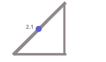
На оставшееся расстояние также приходится — 2.1, так как очевидно:
4.2-2.1=2.1
Это означает, то как в текущий момент времени синус и косинус делят гипотенузу. Поскольку квадрат гипотенузы это 4.2*4.2, то вопрос: что будет если 4.2 умножить на 2.1?! На ту самую её часть, с которой связан один из катетов:
4.2*2.1 = 9, (корень: 3)
Тоже самое для второго катета.
Нашли катеты. И убедились в том, что со времён Пифагора ничего не изменилось.
Далее
Теперь ещё раз осуществим умножение катета А на sin(a), катета B на cos(a).
3*0.7= 2,1
3*0.7 = 2,1
Суммируем:
2.1 + 2.1 =4.2
или
3*0.7 + 3*0.7 =4.2
Снова получили число равное длине удочки… и мы вплотную подобрались к матрице поворота.
Напомню формулу

(изображение из Википедии. Ссылка на статью)
Возьмём её нижнюю часть — получение точки y:
y=x*sin(Ф)+y*cos(Ф)
И сравним с вычислениями выше:
3*0.7 + 3*0.7 = 4.2
y=x*sin(Ф)+y*cos(Ф)
Как две капли воды. Y в нашем случае окажется равным 4.2.
Если применить первую часть формулы к вычислениям, то получим:
3*0.7 — 3*0.7 = 0
Иными словами случится так:
x станет 0 — рыбак поймает леску.
y станет 4.2 — леска сравняется с длиной удочки.
Помним, что для вычисления x синус и косинус меняются местами.
Ф в данном случае равно 45 градусам (Ф = 0.7 ) и при таком угле синус и косинус равны, что удобно для примера. В остальных случаях очевидно величины для синуса и косинуса будут другие. Например, для 40 градусов: cosdegree(40) = 0,7660444431, sindegree(40) = 0,6427876097 (если вы не согласны, обращайтесь в Яндекс, я пользовался его калькулятором).
В итоге
Применяя формулу к новым значениям x,y несколько раз — в цикле, наглядно увидим движение по окружности, каждый раз на 45 градусов.
Если требуется сдвинуть вектор-удочку на один градус, то его и подставляем в формулу на место Ф.
Как происходит вычисление тригонометрических функций?!
Как известно, для вычисления косинуса и синуса угла обычно используются готовые функции. Согласно информации по ссылке вычисление и точность зависят от системы. Для unix-систем есть по крайней мере два варианта: функция, написанная в недрах компании IBM и встроенная инструкция fsin на Ассемблере. Есть также библиотека fdlibm с достаточно наглядным кодом и комментариями, по которым видно, что синус и косинус вычисляются в этой библиотеке через число pi.
А вдруг автор этой статьи все придумал?
Если у вас на компьютере есть веб-сервер и интерпретатор языка PHP, то можно поэкспериментировать со следующим кодом, который вращает блок CSS div:
Файл index.php
Заголовок спойлера
<?php
if (isset($_GET['ok'])) {
$x= $_GET['x']*cos(1)-$y=$_GET['y']*sin(1);
$y= $_GET['x']*sin(1)+$y=$_GET['y']*cos(1);
}
?>
		<style>
			#rotation_martix {
			position: absolute;
			top:  <?=$x+300?>px;
			left: <?=$y+300?>px;
			background-color: #999;
			width: 10px;
			height: 10px;
			}
			</style>
<    div id="rotation_martix">
</  div>
<form  method="GET" >
<input type="submit" name="ok" value="ok">
<input type="text" name="x" value="<?=$x?>">
<input type="text" name="y" value="<?=$y?>">
</form>
Если немного изменить матрицу, то можно получить вращение по спирали или сделать из точки маятник.
Матрица поворота в двумерном пространстве
В
двумерном пространстве поворот можно
описать одним углом
![]()
со
следующей матрицей линейного
преобразования
в декартовой
системе координат:
![]()
Поворот
выполняется путём умножения матрицы
поворота на вектор-столбец,
описывающий вращаемую точку:
![]()
.
Координаты
(x’,y’) в результате поворота точки (x,y)
имеют вид:
![]()
,
![]()
.
Положительным
углам при этом соответствует вращение
вектора против часовой стрелки в обычной,
правосторонней
системе координат,
и по часовой стрелке в левосторонней
системе координат.
[Править] Матрица поворота в трёхмерном пространстве
Матрицами
вращения вокруг оси декартовой
системы координат
на угол α
в трёхмерном пространстве являются:
-
Вращение
вокруг оси x:

,
-
Вращение
вокруг оси y:

,
-
Вращение
вокруг оси z:
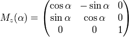
.
Положительным
углам при этом соответствует вращение
вектора против часовой стрелки в правой
системе координат,
и по часовой стрелке в левой системе
координат, если смотреть на плоскость
вращении со стороны полупространства,
где значения координат оси, вокруг
которой осуществляется поворот,
положительные. Правая система координат
связана с выбором правого базиса
(см. правило
буравчика).
Свойства
матрицы поворота.
Свойства матрицы поворота
Если
![]()
—
матрица, задающая поворот вокруг оси
![]()
на
угол ϕ,
то:
-


-

-

-

(след
матрицы
вращения) -

(матрица
имеет единичный определитель). -
если
строки (или столбцы матрицы) рассматривать
как координаты векторов

,
то верны следующие соотношения): -
-
Матрица
обратного поворота получается обычным
транспонированием
матрицы прямого поворота, т. о.

.
-
Алгоритм
Брезенхема для растеризации отрезка.
Алгоритм
Брезенхе́ма
(англ. Bresenham’s
line algorithm)
— это алгоритм, определяющий, какие
точки двумерного
растра нужно закрасить, чтобы получить
близкое приближение прямой линии между
двумя заданными точками.
Это один из старейших алгоритмов в
машинной
графике
— он был разработан Джеком Е. Брезенхэмом
(Jack E. Bresenham) в компании IBM
в 1962
году. Алгоритм широко используется, в
частности, для рисования линий на экране
компьютера. Существует обобщение
алгоритма Брезенхэма
для построения кривых 2-го порядка.
Алгоритм
Отрезок
проводится между двумя точками — (x0,y0)
и (x1,y1),
где в этих парах указаны колонка и
строка, соответственно, номера которых
растут вправо и вниз. Сначала мы будем
предполагать, что наша линия идёт вниз
и вправо, причём горизонтальное расстояние
x1
− x0
превосходит вертикальное y1
− y0,
т.е. наклон линии от горизонтали — менее
45°. Наша цель состоит в том, чтобы для
каждой колонки x
между x0
и x1,
определить, какая строка y
ближе всего к линии, и нарисовать точку
(x,y).
Общая
формула линии между двумя точками:
![]()
Поскольку
мы знаем колонку x,
то строка y
получается округлением к целому
следующего значения:
![]()
Однако,
вычислять точное значение этого выражения
нет необходимости. Достаточно заметить,
что y
растёт от y0
и за каждый шаг мы добавляем к x
единицу и добавляем к y
значение наклона
![]()
которое
можно вычислить заранее. Более того, на
каждом шаге мы делаем одно из двух: либо
сохраняем тот же y,
либо увеличиваем его на 1.
Что
из этих двух выбрать — можно решить,
отслеживая значение
ошибки,
которое означает — вертикальное
расстояние между текущим значением y
и точным значением y
для текущего x.
Всякий раз, когда мы увеличиваем x,
мы увеличиваем значение ошибки на
величину наклона s,
приведённую выше. Если ошибка превысила
0.5, линия стала ближе к следующему y,
поэтому мы увеличиваем y
на единицу, одновременно уменьшая
значение ошибки на 1. В реализации
алгоритма, приведённой ниже, plot(x,y)
рисует точку, а abs
возвращает абсолютную
величину
числа:
function
line(x0, x1, y0, y1)
int
deltax := abs(x1 — x0)
int
deltay := abs(y1 — y0)
real
error := 0
real
deltaerr := deltay / deltax
int
y := y0
for
x from
x0 to
x1
plot(x,y)
error
:= error + deltaerr
if
error >= 0.5
y
:= y + 1
error
:= error — 1.0
Проблема
такого подхода — в том, что с вещественными
величинами, такими как error
и deltaerr,
компьютеры работают относительно
медленно. Кроме того, при вычислениях
с плавающей точкой может накапливаться
ошибка. По этим причинам, лучше работать
только с целыми числами. Это можно
сделать, если умножить все используемые
вещественные величины на deltax.
Единственная проблема — с константой
0.5 — но в данном случае достаточно
умножить обе части неравенства на 2.
Получаем
следующий
код:
function
line(x0, x1, y0, y1)
int
deltax := abs(x1 — x0)
int
deltay := abs(y1 — y0)
int
error := 0
int
deltaerr := deltay
int
y := y0
for
x from
x0 to
x1
plot(x,y)
error
:= error + deltaerr
if
2 * error >= deltax
y
:= y + 1
error
:= error — deltax
Умножение
на 2 для целых чисел реализуется битовым
сдвигом влево.
Теперь
мы можем быстро рисовать линии,
направленные вправо-вниз с величиной
наклона меньше 1. Осталось распространить
алгоритм на рисование во всех направлениях.
Это достигается за счёт зеркальных
отражений, т.е. заменой знака (шаг в 1
заменяется на -1), обменом переменных x
и y,
обменом координат начала отрезка с
координатами конца.
Соседние файлы в предмете [НЕСОРТИРОВАННОЕ]
- #
- #
- #
- #
- #
- #
- #
- #
- #
- #
- #
Матрица, представляющая евклидово вращение
В линейной алгебре матрица вращения — это матрица , которая используется для выполнения поворота в евклидовом пространстве. Например, используя приведенное ниже соглашение, матрица
- R = [cos θ — sin θ sin θ cos θ] { displaystyle R = { begin {bmatrix} cos theta — sin theta \ sin theta cos theta \ end {bmatrix}}}

поворачивает точки в плоскости xy против часовой стрелки на угол θ относительно оси x вокруг начала координат двумерного Декартова система координат. Чтобы выполнить вращение на плоской точке со стандартными координатами v = (x, y), его следует записать как вектор-столбец , а умножить на матрица R:
- R v = [cos θ — sin θ sin θ cos θ] ⋅ [xy] = [x cos θ — y sin θ x sin θ + y cos θ]. { Displaystyle R { textbf {v}} = { begin {bmatrix} cos theta — sin theta \ sin theta cos theta end {bmatrix}} cdot { begin {bmatrix} x \ y end {bmatrix}} = { begin {bmatrix} x cos theta -y sin theta \ x sin theta + y cos theta end {bmatrix}}.}

Примеры в этой статье относятся к активным поворотам векторов против часовой стрелки в правой системе координат (y против часовой стрелки от x) путем предварительного умножения (R слева). Если какой-либо из них изменяется (например, вращающиеся оси вместо векторов, пассивное преобразование ), то следует использовать обратный примерной матрицы, что совпадает с его транспонировать.
Поскольку умножение матриц не влияет на нулевой вектор (координаты начала координат), матрицы вращения описывают повороты вокруг начала координат. Матрицы вращения обеспечивают алгебраическое описание таких вращений и широко используются для вычислений в геометрии, физике и компьютерной графике. В некоторой литературе термин вращение обобщен, чтобы включать неправильные вращения, характеризуемые ортогональными матрицами с детерминантом -1 (вместо +1). Они сочетают правильный поворот с отражениями (которые инвертируют ориентацию ). В других случаях, когда отражения не рассматриваются, метка может быть опущена. В этой статье соблюдается последнее соглашение.
Матрицы поворота — это квадратные матрицы с действительными записями. Более конкретно, их можно охарактеризовать как ортогональные матрицы с определителем 1; то есть квадратная матрица R является матрицей вращения тогда и только тогда, когда R = R и det R = 1. Набор set всех ортогональных матриц размера n с определителем +1 образует группу, известная как специальная ортогональная группа SO (n), одним из примеров которой является группа вращения SO (3). Набор всех ортогональных матриц размера n с определителем +1 или -1 образует (общую) ортогональную группу O (n).
Содержание
- 1 В двух измерениях
- 1.1 Примеры
- 1.2 Направление
- 1.3 Нестандартная ориентация системы координат
- 1.4 Общие повороты
- 1.5 Сложные плоскости в M (2, ℝ)
- 2 В трех измерениях
- 2.1 Основные вращения
- 2.2 Общие вращения
- 2.3 Преобразование из и в угол оси
- 2.3.1 Определение оси
- 2.3.2 Определение угла
- 2.3.3 Матрица поворота от оси и угла
- 3 Свойства
- 4 Примеры
- 5 Геометрия
- 6 Умножение
- 7 Неоднозначности
- 8 Разложения
- 8.1 Независимые плоскости
- 8.2 Последовательные углы
- 8.3 Вложенные измерения
- 8.4 Параметры перекоса по формуле Кэли
- 8.5 Разложение на сдвиги
- 9 Теория групп
- 9.1 Группа Ли
- 9.2 Алгебра Ли
- 9.3 Экспоненциальная карта
- 9.4 Формула Бейкера – Кэмпбелла – Хаусдорфа
- 9.5 Спиновая группа
- 9.6 Бесконечно малые вращения
- 10 Преобразования
- 10.1 Кватернион
- 10.2 Полярное разложение
- 10.3 Ось и угол
- 10.4 Эйлер углы
- 1 0.5 Формулировка вектора в вектор
- 11 Матрицы равномерного случайного вращения
- 12 См. Также
- 13 Примечания
- 14 Примечания
- 15 Ссылки
- 16 Внешние ссылки
В двух измерениях
A поворот вектора на угол θ против часовой стрелки. Вектор изначально выровнен по оси x.
В двух измерениях стандартная матрица вращения имеет следующий вид:
- R (θ) = [cos θ — sin θ sin θ cos θ] { displaystyle R ( theta) = { begin {bmatrix} cos theta — sin theta \ sin theta cos theta \ end {bmatrix}}}.
Это вращается векторы-столбцы посредством следующего умножения матриц,
- [x ′ y ′] = [cos θ — sin θ sin θ cos θ] [xy] { displaystyle { begin {bmatrix} x ‘\ y’ \ end {bmatrix}} = { begin {bmatrix} cos theta — sin theta \ sin theta cos theta \ end {bmatrix}} { begin {bmatrix} x \ y \ end {bmatrix}}}.
 .
.Таким образом, новые координаты (x ′, y ′) точки (x, y) после поворота равны
- Икс ‘= Икс Соз θ — Y грех θ Y’ = Икс грех θ + Y соз θ { Displaystyle { begin {Выровнено} x ‘= x cos theta -y sin theta , \ y ‘= x sin theta + y cos theta , end {align}}}.
 .
.Примеры
Например, когда вектор x ^ = [1 0] { displaystyle mathbf { hat {x}} = { begin {bmatr ix} 1 \ 0 \ end {bmatrix}}} поворачивается на угол θ { displaystyle theta}
 , его новые координаты [соз θ грех θ] { displaystyle { begin {bmatrix} cos theta \ sin theta \ end {bmatrix}}}
 ,
,
и когда вектор y ^ = [ 0 1] { displaystyle mathbf { hat {y}} = { begin {bmatrix} 0 \ 1 \ end {bmatrix}}} повернут на угол θ { displaystyle theta}, его новые координаты: [- sin θ cos θ] { displaystyle { begin {bmatrix} — sin theta \ cos theta \ end {bmatrix}}}
Направление
Направление вращения вектора — против часовой стрелки, если θ положительно (например, 90 °) и по часовой стрелке, если θ отрицательное (например, -90 °). Таким образом, матрица вращения по часовой стрелке находится как
- R (- θ) = [cos θ sin θ — sin θ cos θ] { displaystyle R (- theta) = { begin {bmatrix} cos theta sin theta \ — sin theta cos theta \ end {bmatrix}} ,}.
 .
.Двумерный случай — единственный нетривиальный (т.е. не одномерный) случай, когда группа матриц вращения коммутативна, поэтому не имеет значения, в каком порядке выполняются множественные вращения. Альтернативное соглашение использует вращающиеся оси, и вышеупомянутые матрицы также представляют вращение осей по часовой стрелке на угол θ.
Нестандартная ориентация системы координат
Поворот на угол θ с нестандартными осями.
Если стандартная правосторонняя Декартова система координат, ось x направлена вправо, а ось y — вверх, вращение R (θ) происходит против часовой стрелки. Если используется левая декартова система координат, где x направлен вправо, а y направлен вниз, R (θ) — по часовой стрелке. Такие нестандартные ориентации редко используются в математике, но распространены в компьютерной 2D-графике, которая часто имеет начало в верхнем левом углу и ось Y вниз по экрану или странице.
См. ниже для других альтернативных соглашений, которые могут изменить направление вращения, производимое матрицей вращения.
Обычные вращения
Особенно полезны матрицы [0 — 1 1 0] { displaystyle { begin {bmatrix} 0 -1 \ [3pt] 1 0 \ end {bmatrix}}}![{ displaystyle { begin {bmatrix} 0 -1 \ [3pt] 1 0 \ конец {bmatrix }}}](https://wikimedia.org/api/rest_v1/media/math/render/svg/36535295e7a7d60e9e1b62b5244e00dc2cc984b4) , [- 1 0 0 — 1] { displaystyle { begin {bmatrix} -1 0 \ [3pt] 0 -1 \ end {bmatrix}}}
, [- 1 0 0 — 1] { displaystyle { begin {bmatrix} -1 0 \ [3pt] 0 -1 \ end {bmatrix}}}![{ displaystyle { begin {bmatrix} -1 0 \ [3pt] 0 -1 \ end {bmatrix}}}](https://wikimedia.org/api/rest_v1/media/math/render/svg/6c3cc6953d87e84909de5bd431dd1cba722999a7) , [0 1–1 0] { displaystyle { begin {bmatrix} 0 1 \ [3pt] -1 0 \ end {bmatrix}}}
, [0 1–1 0] { displaystyle { begin {bmatrix} 0 1 \ [3pt] -1 0 \ end {bmatrix}}}![{ displaystyle { begin {bmatrix} 0 1 \ [3pt] -1 0 \ end {bmatrix}}}](https://wikimedia.org/api/rest_v1/media/math/render/svg/249ca88b142a5bb6d56ecbe015474fb5dd10bd6a) для 90 °, 180 ° и 270 ° против часовой стрелки вращения.
для 90 °, 180 ° и 270 ° против часовой стрелки вращения.


 Поворот на 180 ° (в центре) , за которым следует положительный поворот на 90 ° (слева) эквивалентен одиночному отрицательному повороту на 90 ° (положительный 270 °) (справа). Каждая из этих фигур изображает результат вращения относительно вертикального начального положения (внизу слева) и включает в себя матричное представление перестановки, применяемой вращением (в центре справа), а также другие связанные диаграммы. Подробнее см. «Нотация перестановок» в Викиверситете.
Комплексные плоскости в M (2, ℝ)
Так как (0 1 — 1 0) 2 = (- 1 0 0–1), { displaystyle { begin {pmatrix} 0 1 \ — 1 0 end {pmatrix}} ^ {2} = { begin {pmatrix} -1 0 \ 0 -1 end {pmatrix }},} плоскость матриц (xy — yx) { displaystyle { begin {pmatrix} x y \ — y x end {pmatrix}}}
 является изоморфна плоскости комплексных чисел, а указанная выше матрица вращения является точкой на ее единичной окружности, которая действует на плоскости как поворот на θ радиан.
Пусть T = {(a b c — a): a 2 + b c + 1 = 0}. { displaystyle T = {{ begin {pmatrix} a b \ c -a end {pmatrix}}: a ^ {2} + bc + 1 = 0 }.} Это можно показать, что m ∈ T ⟹ m 2 = — 1, { displaystyle m in T подразумевает m ^ {2} = — 1,}
 отрицательное значение единичной матрицы, и п м = {x I + ym: x, y ∈ R} { displaystyle P_ {m} = {xI + ym: x, y in R }}
 — это плоскость матриц, изоморфных ℂ. Тогда согласно формуле Эйлера любое
- g = exp (θ m) = cos (θ) I + m sin (θ) { displaystyle g = exp ( theta m) = cos ( theta) I + m sin ( theta)}— матрица вращения.
 — матрица вращения.
Для получения дополнительных сведений о числовых плоскостях в M (2, ℝ) и их типы поворота см. вещественные матрицы 2 × 2.
В трех измерениях
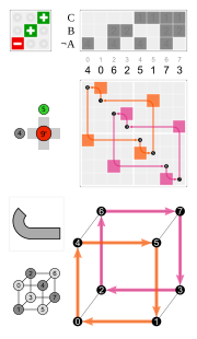

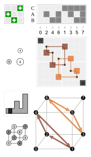 Положительный поворот на 90 ° вокруг оси y (слева) после на один вокруг оси z ( в центре) дает поворот на 120 ° вокруг главной диагонали (справа).. В верхнем левом углу находятся матрицы поворота, в нижнем правом углу — соответствующие перестановки куба с началом координат в его центре.
Базовое вращение
Базовое вращение (также называемое элементарным вращением) — это вращение вокруг одной из осей системы координат. Следующие три основные матрицы поворота поворачивают векторы на угол θ вокруг оси x, y или z в трех измерениях, используя правило правой руки, которое кодирует их чередующиеся знаки. (Эти же матрицы могут также представлять вращение осей по часовой стрелке.)
- R x (θ) = [1 0 0 0 cos θ — sin θ 0 sin θ cos θ] R y (θ) = [соз θ 0 грех θ 0 1 0 — грех θ 0 соз θ] R z (θ) = [соз θ — грех θ 0 грех θ соз θ 0 0 0 1] { displaystyle { begin {alignat} {1} R_ {x} ( theta) = { begin {bmatrix} 1 0 0 \ 0 cos theta — sin theta \ [3pt] 0 sin theta cos theta \ [3pt] end {bmatrix}} \ [6pt] R_ {y} ( theta) = { begin {bmatrix} cos theta 0 sin theta \ [3pt] 0 1 0 \ [3pt] — sin theta 0 cos theta \ end {bmatrix}} \ [6pt] R_ {z} ( theta) = { begin {bmatrix} cos theta — sin theta 0 \ [3pt] sin theta cos theta 0 \ [3pt] 0 0 1 \ end {bmatrix}} end {alignat}}}
Для векторов-столбцов, каждое из этих основных вращений вектора появляется против часовой стрелки, когда ось, вокруг которой они происходят, направлена в сторону наблюдателя, система координат правая, а угол θ положительный. R z, например, будет вращать к оси y вектор, выровненный с осью x, что легко проверить, работая с R z с вектором (1, 0,0):
- R z (90 ∘) [1 0 0] = [cos 90 ∘ — sin 90 ∘ 0 sin 90 ∘ cos 90 ∘ 0 0 0 1] [1 0 0] = [0–1 0 1 0 0 0 0 1] [1 0 0] = [0 1 0] { displaystyle R_ {z} (90 ^ { circ}) { begin {bmatrix} 1 \ 0 \ 0 \ end {bmatrix}} = { begin {bmatrix} cos 90 ^ { circ} — sin 90 ^ { circ} 0 \ sin 90 ^ { circ} quad cos 90 ^ { circ} 0 \ 0 0 1 \ end {bmatrix}} { begin {bmatrix} 1 \ 0 \ 0 \ end {bmatrix}} = { begin {bmatrix} 0 -1 0 1 0 0 \ 0 0 1 \ end {bmatrix}} { begin {bmatrix} 1 \ 0 \ 0 \ end {bmatrix}} = { begin {bmatrix} 0 \ 1 \ 0 \ end {bmatrix}}}
Это похоже на вращение, производимое вышеупомянутой двумерной матрицей вращения. См. ниже для альтернативных соглашений, которые могут явно или фактически изменить направление вращения, производимого этими матрицами.
Общие вращения
Другие матрицы вращения могут быть получены из этих трех с использованием умножения матриц. Например, произведение
- R = R z (α) R y (β) R x (γ) = [cos α — sin α 0 sin α cos α 0 0 0 1] yaw [cos β 0 грех β 0 1 0 — грех β 0 соз β] шаг [1 0 0 0 соз γ — грех γ 0 грех γ соз γ] ролл { Displaystyle R = R_ {z} ( альфа) , R_ {y} ( beta) , R_ {x} ( gamma) = { overset { text {yaw}} { begin {bmatrix} cos alpha — sin alpha 0 \ sin alpha cos alpha 0 \ 0 0 1 \ end {bmatrix}}} { overset { text {pitch}} { begin {bmatrix} cos beta 0 sin beta 0 1 0 \ — sin beta 0 cos beta \ end {bmatrix}}} { overset { text {roll}} { begin {bmatrix} 1 0 0 \ 0 cos gamma — sin gamma \ 0 sin gamma cos gamma \ end {bmatrix}}}
- R = [cos α cos β cos α sin β sin γ — sin α cos γ cos α sin β cos γ + sin α sin γ sin α cos β sin α sin β sin γ + cos α cos γ sin α sin β cos γ — соз α грех γ — грех β соз β грех γ соз β соз γ] { displaystyle R = { begin {bmatrix} cos alpha cos beta cos alpha sin бета грех гамма — грех alpha cos gamma cos alpha sin beta cos gamma + sin alpha sin gamma \ sin alpha cos beta sin alpha sin beta sin gamma + cos alpha cos gamma sin alpha sin beta cos gamma — cos alpha sin gamma \ — sin beta cos beta sin gamma cos beta cos gamma \ end {bmatrix}}}


представляет вращение, углы которого рысканья, тангажа и крена равны α, β и γ соответственно. Более формально это собственное вращение, углы Тейта – Брайана которого равны α, β, γ относительно осей z, y, x, соответственно. Аналогично, произведение
- R = R z (γ) R y (β) R x (α) = [cos γ — sin γ 0 sin γ cos γ 0 0 0 1] [cos β 0 грех β 0 1 0 — грех β 0 соз β] [1 0 0 0 соз α — грех α 0 грех α соз α] { Displaystyle R = R_ {z} ( gamma) , R_ {y} ( beta) , R_ {x} ( alpha) = { begin {bmatrix} cos gamma — sin gamma 0 \ sin gamma cos gamma 0 \ 0 0 1 \ end {bmatrix}} { begin {bmatrix} cos beta 0 sin beta \ 0 1 0 \ — sin beta 0 cos beta \ end {bmatrix}} { begin {bmatrix} 1 0 0 \ 0 cos alpha — sin alpha \ 0 sin alpha cos alpha \ end {bmatrix}}}

представляет собой внешнее вращение, которое (неправильное) Углы Эйлера равны α, β, γ относительно осей x, y, z.
Эти матрицы производят желаемый эффект только в том случае, если они используются для предварительного умножения векторов-столбцов и (поскольку в целом умножение матриц не коммутативное ) только в том случае, если они применяются в указанном порядке (подробнее см. Неоднозначности).
Преобразование из и в угол оси
Каждое вращение в трех измерениях определяется его осью (вектор вдоль этой оси не изменяется при повороте) и его угол — величина вращения вокруг этой оси (теорема вращения Эйлера ).
Существует несколько методов вычисления оси и угла из матрицы вращения (см. Также представление ось – угол ). Здесь мы описываем только метод, основанный на вычислении собственных векторов и собственных значений матрицы вращения. Также можно использовать след матрицы вращения.
Определение оси
Вращение R вокруг оси u может быть разложено с использованием 3 эндоморфизмов P, (I− P) и Q (щелкните, чтобы увеличить).
Учитывая матрицу вращения 3 × 3 R, вектор u, параллельный оси вращения, должен удовлетворять условию
- R u = u, { displaystyle R mathbf {u} = mathbf {u},}
, поскольку вращение u вокруг оси вращения должно приводить к u . Вышеприведенное уравнение может быть решено для u, которое является уникальным с точностью до скалярного множителя, если R = I.
Кроме того, уравнение можно переписать
- R u = I u ⇒ ( R — I) u = 0, { displaystyle R mathbf {u} = I mathbf {u} quad Rightarrow quad (RI) mathbf {u} = 0,}

, что показывает, что u лежит в нулевом пространстве R — I.
С другой стороны, u является собственным вектором R соответствующая собственному значению λ = 1. Каждая матрица вращения должна иметь это собственное значение, два других собственных значения должны быть комплексно сопряженными друг с другом. Отсюда следует, что общая матрица вращения в трех измерениях имеет с точностью до мультипликативной константы только один действительный собственный вектор.
Один из способов определить ось вращения — показать, что:
- 0 = RT 0 + 0 = RT (R — I) u + (R — I) u = (RTR — RT + R — I) U = (I — RT + R — I) u = (R — RT) u { displaystyle { begin {align} 0 = R ^ { mathrm {T}} 0 + 0 \ = R ^ { mathrm {T}} (RI) mathbf {u} + (RI) mathbf {u} \ = left (R ^ { mathrm {T}} RR ^ { mathrm {T}} + RI right) mathbf {u} \ = left (IR ^ { mathrm {T}} + RI right) mathbf {u} \ = left (RR ^ { mathrm {T} } right) mathbf {u} , end {align}}}

Поскольку (R — R) является кососимметричной матрицей, мы можем выбрать u такое, что
- [u] × = (R — RT). { displaystyle [ mathbf {u}] _ { times} = left (RR ^ { mathrm {T}} right).}
![{ displaystyle [ mathbf {u}] _ { times} = left (RR ^ { mathrm {T}} right).}](https://wikimedia.org/api/rest_v1/media/math/render/svg/cd2db19ed794bd4441e4c64300a57a2de7998741)
произведение матрица-вектор становится перекрестным произведением вектора с самим собой, гарантируя, что результат равен нулю:
- (R — RT) u = [u] × u = u × u = 0 { displaystyle left (RR ^ { mathrm {T}} right) mathbf {u} = [ mathbf {u}] _ { times} mathbf {u} = mathbf {u} times mathbf {u} = 0 ,}
![{displaystyle left(R-R^{mathrm {T} }right)mathbf {u} =[mathbf {u} ]_{times }mathbf {u} =mathbf {u} times mathbf {u} =0,}](https://wikimedia.org/api/rest_v1/media/math/render/svg/23c605f4e8ce1a655cdcba0756dd0c62bc4a5a3b)
Следовательно, если
- R = [abcdefghi], { displaystyle R = { begin {bmatrix} a b c \ d e f \ g h i \ end {bmatrix}},}
, затем
- u = [h — fc — гд — б]. { displaystyle mathbf {u} = { begin {bmatrix} hf \ cg \ db \ end {bmatrix}}.}
Величина u, вычисленная таким образом, равна | | u || = 2 sin θ, где θ — угол поворота.
Этот не работает, если R { displaystyle R} симметричен. Выше, если R — R T { displaystyle R-R ^ { mathrm {T}}}
 равно нулю, все последующие шаги недействительны. В этом случае необходимо диагонализовать R { displaystyle R}и найти собственный вектор, соответствующий собственному значению 1.
Определение угла
Чтобы найти угол поворота, когда ось вращения известна, выберите вектор v, перпендикулярный оси. Тогда угол поворота — это угол между v и R v.
. Однако более прямой метод состоит в том, чтобы просто вычислить trace, т. Е. сумма диагональных элементов матрицы вращения. Следует внимательно выбирать правильный знак для угла θ, соответствующий выбранной оси:
- Tr (R) = 1 + 2 cos θ, { displaystyle operatorname {Tr} (R) = 1 + 2 cos theta,}

из чего следует, что абсолютное значение угла равно
- | θ | = arccos (Tr (R) — 1 2). { displaystyle | theta | = arccos left ({ frac { operatorname {Tr} (R) -1} {2}} right).}

Матрица поворота от оси и угла
Матрица собственного поворота R на угол θ вокруг оси u = (ux, uy, uz) { displaystyle mathbf {u} = (u_ {x}, u_ {y}, u_ {z })} , единичный вектор с ux 2 + uy 2 + uz 2 = 1 { displaystyle u_ {x} ^ {2} + u_ {y} ^ {2} + u_ { z} ^ {2} = 1}
 , определяется по формуле:
- R = [cos θ + ux 2 (1 — cos θ) uxuy (1 — cos θ) — uz sin θ uxuz (1 — cos θ) + uy sin θ uyux (1 — cos θ) + uz sin θ cos θ + uy 2 (1 — cos θ) uyuz (1 — cos θ) — ux sin θ uzux (1 — cos θ) — uy sin θ uzuy (1 — cos θ) + ux sin θ cos θ + uz 2 (1 — cos θ)]. { displaystyle R = { begin {bmatrix} cos theta + u_ {x} ^ {2} left (1- cos theta right) u_ {x} u_ {y} left (1- cos theta right) -u_ {z} sin theta u_ {x} u_ {z} left (1- cos theta right) + u_ {y} sin theta \ u_ {y} u_ {x} left (1- cos theta right) + u_ {z} sin theta cos theta + u_ {y} ^ {2} left (1- cos theta right) u_ {y} u_ {z} left (1- cos theta right) -u_ {x} sin theta \ u_ {z} u_ {x} left (1- cos theta справа) -u_ {y} sin theta u_ {z} u_ {y} left (1- cos theta right) + u_ {x} sin theta cos theta + u_ {z} ^ {2} left (1- cos theta right) end {bmatrix}}.}
Вывод этой матрицы из первых принципов можно найти в разделе 9.2 здесь. Основная идея построения этой матрицы — разделить проблему на несколько известных простых шагов.
- Сначала поверните заданную ось и точку так, чтобы ось лежала в одной из координатных плоскостей (xy, yz или zx)
- Затем поверните данную ось и точку так, чтобы ось была выровнена с одна из двух координатных осей для этой конкретной координатной плоскости (x, y или z)
- Используйте одну из основных матриц вращения для поворота точки в зависимости от координатной оси, с которой совмещена ось вращения.
- Обратное вращение пары ось-точка так, чтобы она достигла окончательной конфигурации, как это было на шаге 2 (Отмена шага 2)
- Обратное вращение пары оси-точки, которое было выполнено на шаге 1 (Отмена шаг 1)
Более кратко это можно записать как
- R = (cos θ) I + (sin θ) [u] × + (1 — cos θ) (u ⊗ u), { displaystyle R = ( соз theta) , I + ( sin theta) , [ mathbf {u}] _ { times} + (1- cos theta) , ( mathbf {u} otimes mathbf {u}),}
где [u]×- это матрица перекрестного произведения для u ; выражение u ⊗ u { displaystyle mathbf {u} otimes mathbf {u}} — это внешний продукт, а I — это матрица идентичности. В качестве альтернативы, координаты:
- R jk = {cos 2 θ 2 + sin 2 θ 2 (2 uj 2 — 1), если j = k 2 ujuk sin 2 θ 2 — ε jklul sin θ, если j ≠ К { Displaystyle R_ {jk} = { begin {cases} cos ^ {2} { frac { theta} {2}} + sin ^ {2} { frac { theta} { 2}} left (2u_ {j} ^ {2} -1 right), quad { text {if}} j = k \ 2u_ {j} u_ {k} sin ^ {2} { frac { theta} {2}} — varepsilon _ {jkl} u_ {l} sin theta, quad { text {if}} j neq k end {cases}}}
где ε jkl — символ Леви-Чивиты с ε 123 = 1. Это матричная форма формулы вращения Родригеса, (или эквивалентную, иначе параметризованную формулу Эйлера – Родригеса ) с
- u ⊗ u = uu T = [ux 2 uxuyuxuzuxuyuy 2 uyuzuxuzuyuz 2], [u] × = [0 — uzuyuz 0 — ux — uyux 0]. { displaystyle mathbf {u} otimes mathbf {u} = mathbf {u} mathbf {u} ^ { mathrm {T}} = { begin {bmatrix} u_ {x} ^ {2} u_ {x} u_ {y} u_ {x} u_ {z} \ [3pt] u_ {x} u_ {y} u_ {y} ^ {2} u_ {y} u_ {z} \ [3pt] u_ {x} u_ {z} u_ {y} u_ {z} u_ {z} ^ {2} end {bmatrix}}, qquad [ mathbf {u}] _ { times} = { begin {bmatrix } 0 -u_ {z} u_ {y} \ [3pt] u_ {z} 0 -u_ {x} \ [3pt] -u_ {y} u_ {x} 0 end {bmatrix}}.}
![{ displaystyle mathbf {u} otimes mathbf {u} = mathbf {u} mathbf {u} ^ { mathrm {T}} = { begin {bmatrix} u_ {x} ^ {2} u_ {x} u_ {y} u_ {x} u_ {z} \ [3pt] u_ {x} u_ {y} u_ {y} ^ {2} u_ {y} u_ {z} \ [3pt] u_ {x} u_ {z} u_ {y} u_ {z} u_ {z} ^ {2} end {bmatrix}}, qquad [ mathbf { u}] _ { times} = { begin {bmatrix} 0 -u_ {z} u_ {y} \ [3pt] u_ {z} 0 -u_ {x} \ [3pt] -u_ {y} u_ {x} 0 end {bmatrix}}.}](https://wikimedia.org/api/rest_v1/media/math/render/svg/5d42f590debe54a3015d56b81f1b9de5040f1d35)
В R 3 { displaystyle mathbb {R} ^ {3}}поворот вектора x { displaystyle mathbf {x}} вокруг оси u { displaystyle mathbf {u}}
 на угол θ { displaystyle theta}можно записать как
- Р U (θ) Икс знак равно U (U ⋅ Икс) + соз (θ) (U × X) × U + грех (θ) (U × X) { Displaystyle R _ { mathbf {u}} ( theta) mathbf {x} = mathbf {u} ( mathbf {u} cdot mathbf {x}) + cos left ( theta right) ( mathbf {u} times mathbf {x }) times mathbf {u} + sin left ( theta right) ( mathbf {u} times mathbf {x})}
Если трехмерное пространство правостороннее и θ>0 { displaystyle th eta>0} , это вращение будет происходить против часовой стрелки, когда u указывает на наблюдателя (Правило правой руки ).
Обратите внимание на поразительные просто очевидные отличия от эквивалентной алгебраической формулировки Ли ниже.
Свойства
Для любой n-мерной матрицы вращения R, действующей на ℝ,
- RT = R — 1 { displaystyle R ^ { mathrm {T}} = R ^ {- 1}}(вращение — это ортогональная матрица )
 (вращение — это ортогональная матрица )
. Отсюда следует, что:
- det R = ± 1 { displaystyle det R = pm 1}
Вращение называется правильным, если det R = 1, и неправильным (или поворотным отражением), если det R = –1. Для четных размерностей n = 2k, n собственных значений λ собственного вращения встречаются как пары комплексно сопряженных, которые являются корнями из единицы: λ = e ± i θ j { displaystyle lambda = e ^ { pm i theta _ {j}}} для j = 1,…, k, что реально только для λ = ± 1 { displaystyle lambda = pm 1}
 . Следовательно, не может быть векторов, фиксированных вращением (λ = 1 { displaystyle lambda = 1}
 ), и, следовательно, нет оси вращения. Любые фиксированные собственные векторы встречаются парами, а ось вращения ция — четномерное подпространство.
Для нечетных размеров n = 2k + 1, правильное вращение R будет иметь нечетное количество собственных значений, по крайней мере, с одним λ = 1 { displaystyle lambda = 1}и ось вращения будет подпространством нечетной размерности. Доказательство:
det (R — I) = det (RT) det (R — I) = det (RTR — RT) = det (I — RT) = det (I — R) = (- 1) n det (R — I) = — det (R — I). { Displaystyle { begin {array} {rcl} det (RI) = det (R ^ {T}) det (RI) = det (R ^ {T} ! RR ^ { T}) = det (IR ^ {T}) \ = det (IR) = (-1) ^ {n} det (RI) = — det (RI). end {array}}}
Здесь I — единичная матрица, и мы используем эту det (RT) = det (R) = 1 { displaystyle det (R ^ {T}) = det (R) = 1} , а также (- 1) n = — 1 { displaystyle (-1) ^ {n} = — 1}
 , поскольку n нечетное. Следовательно, det (R — I) = 0, что означает, что существует нулевой вектор v с (R — I) (v ) = 0, то есть R (v ) = v, фиксированный собственный вектор. Также могут быть пары фиксированных собственных векторов в четномерном подпространстве, ортогональном v, поэтому общая размерность фиксированных собственных векторов нечетная.
Например, в 2-пространстве n = 2, поворот на угол θ имеет собственные значения λ = ei θ, e — i θ { displaystyle lambda = e ^ {i theta}, e ^ {- i theta}} , поэтому нет оси вращения, кроме случая, когда θ = 0, в случае нулевого вращения. В 3-пространстве n = 3, ось ненулевого собственного вращения всегда является уникальной линией, а вращение вокруг этой оси на угол θ имеет собственные значения λ = 1, ei θ, е — я θ { displaystyle lambda = 1, e ^ {i theta}, e ^ {- i theta}}
 . В 4-пространстве n = 4 четыре собственных значения имеют вид e ± i θ, e ± i φ { displaystyle e ^ { pm i theta}, e ^ { pm i varphi}}
 . Нулевое вращение имеет θ = φ = 0 { displaystyle theta = varphi = 0}
 . Случай θ = 0, φ ≠ 0 { displaystyle theta = 0, varphi neq 0}
 называется простым вращением с двумя единичными собственными значениями, образующими плоскость оси, и двумерное вращение, ортогональное плоскости оси. В противном случае осевая плоскость отсутствует. Случай θ = φ { displaystyle theta = varphi}
 называется изоклиническим вращением, имеющим собственные значения e ± i θ { displaystyle e ^ { pm i theta }}
 , каждый повторяется дважды, поэтому каждый вектор поворачивается на угол θ.
След матрицы вращения равен сумме ее собственных значений. При n = 2 поворот на угол θ имеет след 2 cos θ. При n = 3 поворот вокруг любой оси на угол θ имеет след 1 + 2 cos θ. Для n = 4 и след равен 2 (cos θ + cos φ) { displaystyle 2 ( cos theta + cos varphi)} , что превращается в 4 cos θ для изоклинного вращения.
Примеры
|
|


Geometry
В евклидовой геометрии вращение является примером изометрии, преобразования, которое перемещает точки без изменения расстояний между ними. Вращения отличаются от других изометрий двумя дополнительными свойствами: они оставляют (по крайней мере) одну точку фиксированной, и они оставляют неизменным «хиральность «. Напротив, смещение перемещает каждую точку, отражение меняет порядок левого и правого, скользящее отражение делает и то, и другое, а неправильное вращение сочетает изменение руки с нормальным вращением.
Если фиксированная точка берется за начало декартовой системы координат, то каждой точке могут быть заданы координаты как смещение от начала координат. Таким образом, вместо самих точек можно работать с векторным пространством смещений. Теперь предположим (p 1,…, p n) — координаты вектора p от начала O до точки P. Выберите ортонормированный база для наших координат; тогда квадрат расстояния до P по Пифагору равен
- d 2 (O, P) = ‖ p ‖ 2 = ∑ r = 1 npr 2 { displaystyle d ^ {2} (O, P) = | mathbf {p} | ^ {2} = sum _ {r = 1} ^ {n} p_ {r} ^ {2}}
, которое можно вычислить с помощью умножения матриц
- ‖ p ‖ 2 = [p 1 ⋯ pn] [p 1 ⋮ pn] = p T p. { displaystyle | mathbf {p} | ^ {2} = { begin {bmatrix} p_ {1} cdots p_ {n} end {bmatrix}} { begin {bmatrix} p_ {1} \ vdots \ p_ {n} end {bmatrix}} = mathbf {p} ^ { mathrm {T}} mathbf {p}.}

Геометрическое вращение преобразует линии в линии и сохраняет соотношения расстояний между точками. Из этих свойств можно показать, что вращение является линейным преобразованием векторов и, таким образом, может быть записано в форме матрицы, Q p . Тот факт, что при повороте сохраняются не только отношения, но и сами расстояния, определяется как
- p T p = (Q p) T (Q p), { displaystyle mathbf {p} ^ { mathrm {T} } mathbf {p} = (Q mathbf {p}) ^ { mathrm {T}} (Q mathbf {p}),}

или
- p TI p = (p TQT) (Q р) = р Т (QTQ) р. { displaystyle { begin {align} mathbf {p} ^ { mathrm {T}} I mathbf {p} {} = left ( mathbf {p} ^ { mathrm {T}} Q ^ { mathrm {T}} right) (Q mathbf {p}) \ {} = mathbf {p} ^ { mathrm {T}} left (Q ^ { mathrm {T}} Q right) mathbf {p}. end {align}}}

Поскольку это уравнение выполняется для всех векторов, p, можно сделать вывод, что каждая матрица поворота Q удовлетворяет ортогональности условие,
- QTQ = I. { displaystyle Q ^ { mathrm {T}} Q = I.}

Вращения сохраняют ручность, потому что они не могут изменить порядок осей, что подразумевает условие специальной матрицы,
- det Q = + 1. { displaystyle det Q = + 1.}
Что не менее важно, можно показать, что любая матрица, удовлетворяющая этим двум условиям, действует как вращение.
Умножение
Инверсией матрицы вращения является ее транспонирование, которое также является матрицей вращения:
- (QT) T (QT) = QQT = I det QT = det Q = + 1. { displaystyle { begin {align} left (Q ^ { mathrm {T}} right) ^ { mathrm {T}} left (Q ^ { mathrm {T}} right) = QQ ^ { mathrm {T}} = I \ det Q ^ { mathrm {T}} = det Q = + 1. End {align}}}

Произведение двух вращений matrices — матрица вращения:
- (Q 1 Q 2) T (Q 1 Q 2) = Q 2 T (Q 1 TQ 1) Q 2 = I det (Q 1 Q 2) = (det Q 1) ( det Q 2) = + 1. { displaystyle { begin {align} left (Q_ {1} Q_ {2} right) ^ { mathrm {T}} left (Q_ {1} Q_ {2} right) = Q_ {2} ^ { mathrm {T}} left (Q_ {1} ^ { mathrm {T}} Q_ {1} right) Q_ {2} = I \ det left (Q_ {1} Q_ {2} right) = left ( det Q_ {1} right) left ( det Q_ {2} right) = + 1. end {align}}}

Для n>2 умножение матриц вращения n × n обычно не коммутативное.
- Q 1 = [0 — 1 0 1 0 0 0 0 1] Q 2 = [0 0 1 0 1 0 — 1 0 0] Q 1 Q 2 = [0 — 1 0 0 0 1 — 1 0 0] Q 2 Q 1 = [0 0 1 1 0 0 0 1 0]. { displaystyle { begin {align} Q_ {1} = { begin {bmatrix} 0 -1 0 \ 1 0 0 \ 0 0 1 end {bmatrix}} Q_ {2} = { begin {bmatrix} 0 0 1 0 1 0 \ — 1 0 0 end {bmatrix}} \ Q_ {1} Q_ {2} = { begin {bmatrix} 0 -1 0 \ 0 0 1 \ — 1 0 0 end {bmatrix}} Q_ {2} Q_ {1} = { begin {bmatrix} 0 0 1 \ 1 0 0 \ 0 1 0 end {bmatrix}}. End {align}}}
Обратите внимание, что любая единичная матрица является вращением матрица, и это матричное умножение является ассоциативным, мы можем суммировать все эти свойства, сказав, что матрицы вращения n × n образуют группу, которая для n>2 не -абелева, называемая специальной ортогональной группой и обозначаемая SO (n), SO (n, R ), SO n или SO n(R) группа матриц вращения n × n изоморфна группе вращений в n-мерном пространстве. Это означает, что умножение матриц вращения соответствует композиции вращений, применяемых в порядке слева направо соответствующих матриц.
Неоднозначности
Псевдонимы и вращения алиби
Интерпретация матрицы вращения может быть предметом многих неоднозначностей.
В большинстве случаев эффект неоднозначности эквивалентен эффекту поворота матрицы инверсия (для этих ортогональных матриц эквивалентно матрице транспонировать ).
- Преобразование псевдонима или алиби (пассивного или активного)
- Координаты точки P могут измениться из-за поворота системы координат CS (псевдоним ), или поворот точки P (алиби ). В последнем случае вращение P также производит вращение вектора v, представляющего P. Другими словами, либо P и v фиксированы, в то время как CS вращается (псевдоним), либо CS фиксируется, а P и v вращаются (алиби). Любое данное вращение может быть законно описано в обоих направлениях, поскольку векторы и системы координат фактически вращаются относительно друг друга, вокруг одной оси, но в противоположных направлениях. В этой статье мы выбрали подход алиби для описания вращений. Например,
- R (θ) = [соз θ — грех θ sin θ cos θ] { displaystyle R ( theta) = { begin {bmatrix} cos theta — sin theta \ sin theta cos theta \ end {bmatrix}}}
- R (θ) = [соз θ — грех θ sin θ cos θ] { displaystyle R ( theta) = { begin {bmatrix} cos theta — sin theta \ sin theta cos theta \ end {bmatrix}}}
- представляет собой поворот вектора v против часовой стрелки на угол θ или поворот CS с помощью тот же угол, но в противоположном направлении (т.е. по часовой стрелке). Преобразования алиби и псевдонима также известны как активные и пассивные преобразования соответственно.
- Преумножение или постумножение
- Одна и та же точка P может быть представлена либо вектор-столбец vили вектор-строка w. Матрицы поворота могут либо до умножения векторов-столбцов (R v ), либо после умножения векторов-строк (w R). Однако R v производит вращение в противоположном направлении относительно w R. В этой статье вращения, производимые на векторах-столбцах, описаны с помощью предварительного умножения. Чтобы получить точно такое же вращение (т. Е. Те же конечные координаты точки P), вектор-строку необходимо умножить на транспонирование R (то есть w R).
- Правосторонние или левосторонние координаты
- Матрица и вектор могут быть представлены в правой или левой системе координат. На протяжении всей статьи мы предполагали правую ориентацию, если не указано иное.
- Векторы или формы
- В векторном пространстве есть двойное пространство из линейных форм, и матрица может действовать как на векторы, так и на формы.
Разложения
Независимые плоскости
Рассмотрим матрицу вращения 3 × 3
- Q = [0,36 0,48 — 0,80 — 0,80 0,60 0,00 0,48 0,64 0,60]. { displaystyle Q = { begin {bmatrix} 0,36 0,48 -0,80 \ — 0,80 0,60 0,00 \ 0,48 0,64 0,60 end {bmatrix}}.}
Если Q действует в определенное направление, v, просто как масштабирование на коэффициент λ, тогда мы имеем
- Q v = λ v, { displaystyle Q mathbf {v} = lambda mathbf {v}, }
так, что
- 0 = (λ I — Q) v. { displaystyle mathbf {0} = ( lambda IQ) mathbf {v}.}
Таким образом, λ является корнем характеристического многочлена для Q,
- 0 = det (λ I — Q) = λ 3 — 39 25 λ 2 + 39 25 λ — 1 = (λ — 1) (λ 2 — 14 25 λ + 1). { displaystyle { begin {align} 0 {} = det ( lambda IQ) \ {} = lambda ^ {3} — { tfrac {39} {25}} lambda ^ {2} + { tfrac {39} {25}} lambda -1 \ {} = ( lambda -1) left ( lambda ^ {2} — { tfrac {14} {25}} lambda +1 right). end {align}}}
Следует отметить две особенности. Во-первых, один из корней (или собственных значений ) равен 1, что говорит нам о том, что матрица не влияет на какое-то направление. Для вращения в трех измерениях это ось вращения (концепция, не имеющая значения ни в каком другом измерении). Во-вторых, два других корня представляют собой пару комплексно сопряженных корней, произведение которых равно 1 (постоянный член квадратичного), а сумма равна 2 cos θ (отрицательный линейный член). Эта факторизация представляет интерес для матриц вращения 3 × 3, потому что для всех них происходит одно и то же. (В качестве особых случаев для нулевого поворота оба «комплексно сопряженных» значения равны 1, а для поворота на 180 ° они оба равны -1.) Кроме того, аналогичная факторизация выполняется для любой матрицы вращения n × n. Если размерность n нечетная, будет «висящее» собственное значение 1; и для любой размерности остальная часть полинома делится на квадратичные члены, подобные приведенному здесь (с двумя отмеченными частными случаями). Гарантируется, что характеристический многочлен будет иметь степень n и, следовательно, n собственных значений. А поскольку матрица вращения коммутирует со своим транспонированием, это нормальная матрица , поэтому ее можно диагонализовать. Мы заключаем, что каждая матрица вращения, когда она выражена в подходящей системе координат, разбивается на независимые вращения двумерных подпространств, не более n / 2 из них.
Сумма элементов на главной диагонали матрицы называется трассой ; он не меняется, если мы переориентируем систему координат, и всегда равен сумме собственных значений. Это имеет удобный вывод для матриц вращения 2 × 2 и 3 × 3, что след показывает угол поворота, θ, в двумерном пространстве (или подпространстве). Для матрицы 2 × 2 след равен 2 cos θ, а для матрицы 3 × 3 — 1 + 2 cos θ. В трехмерном случае подпространство состоит из всех векторов, перпендикулярных оси вращения (инвариантное направление с собственным значением 1). Таким образом, мы можем извлечь из любой матрицы вращения 3×3 ось вращения и угол, и они полностью определяют вращение.
Последовательные углы
Ограничения на матрицу поворота 2 × 2 подразумевают, что она должна иметь форму
- Q = [a — bba] { displaystyle Q = { begin {bmatrix } a -b \ b a end {bmatrix}}}
с a + b = 1. Следовательно, мы можем установить a = cos θ и b = sin θ для некоторого угла θ. Чтобы решить для θ, недостаточно смотреть только на a или на b; мы должны рассмотреть оба вместе, чтобы разместить угол в правильном квадранте , используя функцию арктангенса с двумя аргументами.
Теперь рассмотрим первый столбец матрицы вращения 3 × 3,
- [a b c]. { displaystyle { begin {bmatrix} a \ b \ c end {bmatrix}}.}
Хотя a + b, вероятно, будет не равным 1, но некоторое значение r < 1, we can use a slight variation of the previous computation to find a so-called вращение Гивенса, которое преобразует столбец в
- [r 0 c], { displaystyle { begin {bmatrix} r \ 0 \ c end {bmatrix}},}
обнуление b. Это действует на подпространство, натянутое на оси x и y. Затем мы можем повторить процесс для xz-подпространства до нуля c. Действуя на полную матрицу, эти два поворота образуют схематический вид
- Q x z Q x y Q = [1 0 0 0 ∗ ∗ 0 ∗ ∗]. { displaystyle Q_ {xz} Q_ {xy} Q = { begin {bmatrix} 1 0 0 \ 0 ast ast \ 0 ast ast end {bmatrix}}.}
Перемещение внимания на во втором столбце поворот Гивенса yz-подпространства теперь может обнулить значение z. Это приводит полную матрицу к форме
- Q yz Q xz Q xy Q = [1 0 0 0 1 0 0 0 1], { displaystyle Q_ {yz} Q_ {xz} Q_ {xy} Q = { begin {bmatrix} 1 0 0 \ 0 1 0 \ 0 0 1 end {bmatrix}},}
которая является единичной матрицей. Таким образом, мы разложили Q как
- Q = Q x y — 1 Q x z — 1 Q y z — 1. { displaystyle Q = Q_ {xy} ^ {- 1} Q_ {xz} ^ {- 1} Q_ {yz} ^ {- 1}.}
Матрица вращения n × n будет иметь (n — 1) + (n — 2) + ⋯ + 2 + 1, или
- ∑ k = 1 n — 1 k = n (n — 1) 2 { displaystyle sum _ {k = 1} ^ {n-1} k = { frac {n (n-1)} {2}}}

элементов ниже диагонали до нуля. Мы можем обнулить их, расширив ту же идею прохождения по столбцам с серией вращений в фиксированной последовательности плоскостей. Мы заключаем, что набор матриц вращения n × n, каждая из которых имеет n элементов, может быть параметризовано n (n − 1) / 2 углами.
| xzx w | xzy w | xyx w | xyz w |
| yxy w | yxz w | yzy w | yzx w |
| zyz w | zyx w | zxz w | zxy w |
| xzx b | yzx b | xyx b | zyx b |
| yxy b | zxy b | yzy b | xzy b |
| zyz b | xyz b | zxz b | yxz b |
In в трех измерениях это переформулирует в матричной форме наблюдение, сделанное Эйлером, поэтому математики называют упорядоченную последовательность трех углов углами Эйлера. Однако ситуация несколько сложнее, чем мы до сих пор указывали. Несмотря на небольшой размер, у нас действительно есть значительная свобода в последовательности используемых пар осей; и у нас также есть некоторая свобода в выборе углов. Таким образом, мы находим много различных соглашений, используемых при параметризации трехмерного вращения для физики, медицины, химии или других дисциплин. Когда мы включаем опцию мировых осей или осей тела, возможны 24 различных последовательности. И хотя некоторые дисциплины называют любую последовательность углами Эйлера, другие дают разные названия (Кардано, Тейт – Брайан, крен-тангаж-рыскание ) различным последовательностям.
Одна из причин большого количества опций заключается в том, что, как отмечалось ранее, вращения в трех измерениях (и выше) не меняются. Если мы перевернем заданную последовательность вращений, мы получим другой результат. Это также означает, что мы не можем составить два поворота, сложив их соответствующие углы. Таким образом, углы Эйлера не являются векторами, несмотря на внешнее сходство в виде тройки чисел.
Вложенные измерения
Матрица вращения 3 × 3, например
- Q 3 × 3 = [cos θ — sin θ 0 sin θ cos θ 0 0 0 1] { displaystyle Q_ {3 times 3} = { begin {bmatrix} cos theta — sin theta { color {CadetBlue} 0} \ sin theta cos theta { color {CadetBlue} 0} \ { color {CadetBlue} 0} { color {CadetBlue} 0} { color {CadetBlue} 1} end {bmatrix}}}
предлагает поворот 2 × 2 матрица,
- Q 2 × 2 = [соз θ — грех θ грех θ соз θ], { displaystyle Q_ {2 times 2} = { begin {bmatrix} cos theta — sin theta \ sin theta cos theta end {bmatrix}},}
вставляется в левый верхний угол:
- Q 3 × 3 = [Q 2 × 2 0 0 T 1 ]. { Displaystyle Q_ {3 times 3} = left [{ begin {matrix} Q_ {2 times 2} mathbf {0} \ mathbf {0} ^ { mathrm {T}} 1 end {matrix}} right].}
![{ displaystyle Q_ {3 times 3} = left [{ begin {matrix} Q_ {2 times 2} mathbf {0} \ mathbf {0} ^ { mathrm {T}} 1 end {matrix}} right].}](https://wikimedia.org/api/rest_v1/media/math/render/svg/8cadc2fd9165c4118b5529cd11c9a4349b9ba453)
Это не иллюзия; не одна, а множество копий n-мерных вращений находятся внутри (n + 1) -мерных вращений, как подгруппы. Каждое вложение оставляет фиксированным одно направление, которое в случае матриц 3 × 3 является осью вращения. Например, мы имеем
- Q x (θ) = [1 0 0 0 cos θ — sin θ 0 sin θ cos θ], Q y (θ) = [cos θ 0 sin θ 0 1 0 — грех θ 0 соз θ], Q z (θ) = [соз θ — грех θ 0 грех θ соз θ 0 0 0 1], { displaystyle { begin {align} Q_ { mathbf {x}} ( theta) = { begin {bmatrix} { color {CadetBlue} 1} { color {CadetBlue} 0} { color {CadetBlue} 0} \ { color { CadetBlue} 0} cos theta — sin theta \ { color {CadetBlue} 0} sin theta cos theta end {bmatrix}}, \ [8px] Q _ { mathbf {y}} ( theta) = { begin {bmatrix} cos theta { color {CadetBlue} 0} sin theta \ { color {CadetBlue} 0} { color { CadetBlue} 1} { color {CadetBlue} 0} \ — sin theta { color {CadetBlue} 0} cos theta end {bmatrix}}, \ [8px] Q _ { mathbf {z}} ( theta) = { begin {bmatrix} cos theta — sin theta { color {CadetBlue} 0} \ sin theta cos theta { color {CadetBlue} 0} \ { color {CadetBlue} 0} { color {CadetBlue} 0} { color {CadetBlue} 1} end {bmatrix}}, end {align}}}
фиксация оси x, оси y и оси z, соответственно ely. Ось вращения не обязательно должна быть координатной осью; если u = (x, y, z) — единичный вектор в желаемом направлении, то
- Q u (θ) = [0 — zyz 0 — x — yx 0] sin θ + (I — uu T) cos θ + uu T = [(1 — x 2) c θ + x 2 — zs θ — xyc θ + xyys θ — xzc θ + xzzs θ — xyc θ + xy (1 — y 2) c θ + y 2 — xs θ — yzc θ + yz — ys θ — xzc θ + xzxs θ — yzc θ + yz (1 — z 2) c θ + z 2] = [x 2 (1 — c θ) + c θ xy (1 — c θ) — zs θ xz (1 — c θ) + ys θ xy (1 — c θ) + zs θ y 2 (1 — c θ) + c θ yz (1 — c θ) — xs θ xz (1 — c θ) — ys θ yz (1 — c θ) + xs θ z 2 (1 — c θ) + c θ], { displaystyle { begin {align} Q _ { mathbf {u}} ( theta) = { begin {bmatrix} 0 -z y \ z 0 -x \ — y x 0 end {bmatrix}} sin theta + left (I- mathbf {u} mathbf {u} ^ { mathrm {T}} right) cos theta + mathbf {u} mathbf {u} ^ { mathrm {T}} \ [8px] = { begin {bmatrix } left (1-x ^ {2} right) c _ { theta} + x ^ {2} — zs _ { theta} -xyc _ { theta} + xy ys _ { theta} -xzc _ { theta} + xz \ zs _ { theta} -xyc _ { theta} + xy left (1-y ^ {2} right) c _ { theta} + y ^ {2} — xs _ { theta} -yzc _ { theta} + yz \ — ys _ { theta} -xzc _ { theta} + xz xs _ { theta} -yzc _ { theta} + yz left (1-z ^ {2} right) c _ { theta} + z ^ {2} end {bmatrix}} \ [8px] = { begin {bmatrix} x ^ {2} (1- c _ { theta}) + c _ { theta} xy (1-c _ { theta}) — zs _ { theta} xz (1-c _ { theta}) + ys _ { theta} \ xy (1- c _ { theta}) + zs _ { theta} y ^ {2} (1-c _ { theta}) + c _ { theta} yz (1-c _ { theta}) — xs _ { theta} \ xz (1-c _ { theta}) — ys _ { theta} yz (1-c _ { theta}) + xs _ { theta} z ^ {2} (1-c _ { theta}) + c _ { theta} end {bmatrix}}, end {align}}}
![{ displaystyle { begin {align} Q _ { mathbf {u}} ( theta) = { begin {bmatrix} 0 -z y \ z 0 -x \ - y x 0 end {bmatrix}} sin theta + left (I- mathbf {u} mathbf {u} ^ { mathrm {T}} right) cos theta + mathbf {u} mathbf {u} ^ { mathrm {T}} \ [8px] = { begin { bmatrix} left (1-x ^ {2} right) c _ { theta} + x ^ {2} - zs _ { thet a} -xyc _ { theta} + xy ys _ { theta} -xzc _ { theta} + xz \ zs _ { theta} -xyc _ { theta} + xy left (1-y ^ {2} right) c _ { theta} + y ^ {2} - xs _ { theta} -yzc _ { theta} + yz \ - ys _ { theta} -xzc _ { theta} + xz xs _ { theta} -yzc _ { theta} + yz left (1-z ^ {2} right) c _ { theta} + z ^ {2} end {bmatrix}} \ [8px] = { begin {bmatrix} x ^ { 2} (1-c _ { theta}) + c _ { theta} xy (1-c _ { theta}) - zs _ { theta} xz (1-c _ { theta}) + ys _ { theta} xy (1-c _ { theta}) + zs _ { theta} y ^ {2} (1-c _ { theta}) + c _ { theta} yz (1-c _ { theta}) - xs_ { theta} \ xz (1-c _ { theta}) - ys _ { theta} yz (1-c _ { theta}) + xs _ { theta} z ^ {2} (1-c _ { theta}) + c _ { theta} end {bmatrix}}, end {align}}}](https://wikimedia.org/api/rest_v1/media/math/render/svg/5e7d7b2324e80c2a1b73f7091e84ad670f75c3ea)
где c θ = cos θ, s θ = sin θ, это поворот на угол θ оставшаяся ось u исправлена.
Направление в (n + 1) -мерном пространстве будет вектором единичной величины, который мы можем рассматривать как точку на обобщенной сфере S. Таким образом, естественно описать группу вращений SO (n + 1) как объединение SO (n) и S. Подходящим формализмом является пучок волокон,
- SO (n) ↪ SO (n + 1) → S n, { displaystyle SO (n) hookrightarrow SO ( n + 1) to S ^ {n},}
где для каждого направления в базовом пространстве S слой над ним в общем пространстве SO (n + 1) является копией пространства слоев, SO (n), а именно вращения, которые сохраняют это направление фиксированным.
Таким образом, мы можем построить матрицу вращения n × n, начав с матрицы 2 × 2, направив ее фиксированную ось на S (обычная сфера в трехмерном пространстве), нацелив получившееся вращение на S, и так далее до S. Точка на S может быть выбрана с помощью n чисел, поэтому у нас снова есть n (n — 1) / 2 чисел для описания любой матрицы вращения n × n.
Фактически, мы можем рассматривать последовательное угловое разложение, обсуждавшееся ранее, как обращение этого процесса. Композиция из n — 1 поворотов Гивенса приводит первый столбец (и строку) к (1,0,…, 0), так что оставшаяся часть матрицы представляет собой матрицу вращения размерности на единицу меньше, встроенную так, чтобы оставить (1, 0,…, 0) исправлено.
Параметры перекоса по формуле Кэли
Когда матрица вращения Q размером n × n не включает собственное значение −1, то есть ни одно из плоских вращений, которые она включает, не является поворотом на 180 °, тогда Q + I — это обратимая матрица. Большинство матриц вращения соответствуют этому описанию, и для них можно показать, что (Q — I) (Q + I) является кососимметричной матрицей, A. Таким образом, A = −A; и поскольку диагональ обязательно равна нулю, и поскольку верхний треугольник определяет нижний, A содержит 1 / 2n (n — 1) независимых чисел.
Удобно, что I — A обратимо, если A кососимметрична; таким образом, мы можем восстановить исходную матрицу, используя преобразование Кэли,
- A ↦ (I + A) (I — A) — 1, { displaystyle A mapsto (I + A) (IA) ^ {- 1 },}
, который отображает любую кососимметричную матрицу A в матрицу вращения. Фактически, за исключением отмеченных исключений, таким способом мы можем создать любую матрицу вращения. Хотя в практических приложениях мы вряд ли можем позволить себе игнорировать поворот на 180 °, преобразование Кэли по-прежнему является потенциально полезным инструментом, позволяющим параметризовать большинство матриц поворота без тригонометрических функций.
В трех измерениях, например, мы имеем (Cayley 1846)
- [0 — zyz 0 — x — yx 0] ↦ 1 1 + x 2 + y 2 + z 2 [1 + x 2 — y 2 — z 2 2 xy — 2 z 2 y + 2 xz 2 xy + 2 z 1 — x 2 + y 2 — z 2 2 yz — 2 x 2 xz — 2 y 2 x + 2 yz 1 — x 2 — y 2 + z 2]. { displaystyle { begin {align} { begin {bmatrix} 0 -z y \ z 0 -x \ — y x 0 end {bmatrix}} mapsto \ [3pt ] quad { frac {1} {1 + x ^ {2} + y ^ {2} + z ^ {2}}} { begin {bmatrix} 1 + x ^ {2} -y ^ {2 } -z ^ {2} 2xy-2z 2y + 2xz \ 2xy + 2z 1-x ^ {2} + y ^ {2} -z ^ {2} 2yz-2x \ 2xz-2y 2x + 2yz 1-x ^ {2 } -y ^ {2} + z ^ {2} end {bmatrix}}. end {align}}}
Если мы сжимаем элементы перекоса в вектор (x, y, z), тогда мы произвести поворот на 90 ° вокруг оси x для (1, 0, 0), вокруг оси y для (0, 1, 0) и вокруг оси z для (0, 0, 1). Повороты на ° просто недосягаемы; поскольку в пределе x → ∞ (x, 0, 0) действительно приближается к повороту на 180 ° вокруг оси x, и аналогично для других направлений.
Разложение на shears
Для 2D-случая матрица вращения может быть разложен на три матрицы сдвига (Paeth 1986):
- R (θ) = [1 — tan θ 2 0 1] [1 0 sin θ 1] [1 — загар θ 2 0 1] { displaystyle { begin {align} R ( theta) {} = { begin {bmatrix} 1 — tan { frac { theta} {2}} \ 0 1 end {bmatrix}} { begin {bmatrix} 1 0 \ sin theta 1 end {bmatrix}} { begin {bmatrix} 1 — tan { frac { theta} {2}} \ 0 1 end {bmatrix}} end {align}}}
Это полезно, например, в компьютерной графике, поскольку сдвиги могут быть реализованы с меньшим количеством инструкций умножения, чем прямое вращение растрового изображения. На современных компьютерах это может не иметь значения, но может быть актуальным для очень старых или недорогих микропроцессоров.
Поворот также можно записать как два сдвига и масштабирование (Daubechies Sweldens 1998):
- R (θ) = [1 0 тангенса θ 1] [1 — грех θ соз θ 0 1] [соз θ 0 0 1 соз θ] { displaystyle { begin {align} R ( theta) {} = { begin {bmatrix} 1 0 \ tan theta 1 end {bmatrix}} { begin {bmatrix} 1 — sin theta cos theta \ 0 1 end {bmatrix}} { begin {bmatrix} cos theta 0 0 { frac {1} { cos theta}} end {bmatrix}} end {align}}}
Теория групп
Ниже приведены некоторые основные факты о роли коллекции всех матриц вращения фиксированной размерности (здесь в основном 3) в математике и особенно в физике, где симметрия вращения является требованием каждого истинно фундаментального закона (из-за предположения об изотропии пространства ), и где та же самая симметрия, если она присутствует, является упрощающим свойством многих проблем менее фундаментального характера. Примеры изобилуют классической механикой и квантовой механикой. Знание части решений, относящихся к этой симметрии, применимо (с определенными оговорками) ко всем таким проблемам, и это может быть исключено из конкретной проблемы, что снижает ее сложность. Ярким примером — в математике и физике — может быть теория сферических гармоник. Их роль в теории групп групп вращений состоит в том, что они являются пространством представления для всего множества конечномерных неприводимых представлений группы вращений SO (3). По этой теме см. Группа вращения SO (3) § Сферические гармоники.
Для получения более подробной информации см. Основные статьи, перечисленные в каждом подразделе.
Группа Ли
Матрицы вращения n × n для каждого n образуют группу , специальную ортогональную группу, SO (n). Эта алгебраическая структура сочетается с топологической структурой, унаследованной от GL n (ℝ) таким образом, что операции умножения и обратного преобразования равны аналитические функции элементов матрицы. Таким образом, SO (n) для каждого n является группой Ли. Это компактный и соединенный, но не односвязный. Это также полупростая группа, фактически простая группа за исключением SO (4). Актуальность этого состоит в том, что все теоремы и весь аппарат из теории аналитических многообразий (аналитические многообразия, в частности, гладкие многообразия ) применимы, а хорошо разработанная теория представлений компактных полу- простые группы готовы к использованию.
Алгебра Ли
Алгебра Ли so (n) SO (n) задается как
- so (n) = o (n) = {X ∈ M n (R) | Икс = — XT}, { displaystyle { mathfrak {so}} (n) = { mathfrak {o}} (n) = left {X in M_ {n} ( mathbb {R}) left | X = -X ^ { mathrm {T}} right } right.,}

и является пространством кососимметричных матриц размерности n, см. классическая группа, где o (n) — это алгебра Ли O (n), ортогональной группы. Для справки, наиболее распространенной основой для, поэтому (3) является
- L x = [0 0 0 0 0 — 1 0 1 0], L y = [0 0 1 0 0 0 — 1 0 0], L z = [0 — 1 0 1 0 0 0 0 0]. { displaystyle L _ { mathbf {x}} = left [{ begin {matrix} 0 0 0 \ 0 0 -1 \ 0 1 0 end {matrix}} right], quad L _ { mathbf {y}} = left [{ begin {matrix} 0 0 1 \ 0 0 0 \ — 1 0 0 end {matrix}} right], quad L _ { mathbf {z}} = left [{ begin {matrix} 0 — 1 0 \ 1 0 0 \ 0 0 0 end {matrix}} right].}
![{ displaystyle L _ { mathbf {x} } = left [{ begin {matrix} 0 0 0 \ 0 0 -1 \ 0 1 0 end {matrix}} right], quad L _ { mathbf {y}} = left [{ begin {matrix} 0 0 1 \ 0 0 0 \ - 1 0 0 end {matrix}} right], quad L _ { mathbf {z}} = left [{ begin {matrix} 0 -1 0 \ 1 0 0 \ 0 0 0 0 end { матрица}} right].}](https://wikimedia.org/api/rest_v1/media/math/render/svg/28dc52862f27a921458ac450755300149dca13f5)
Экспоненциальное отображение
Соединение алгебры Ли с группой Ли — это экспоненциальное отображение, которое является определяется с использованием стандартной матрицы экспоненциальной серии для e Для любой кососимметричной матрицы A, exp (A) всегда является матрицей вращения.
Важным практическим примером является корпус 3 × 3. В группе вращений SO (3) показано, что можно идентифицировать каждый A ∈, поэтому (3) с вектором Эйлера ω = θ u, где u = (x, y, z) — вектор единичной величины.
По свойствам идентификации su (2) ≅ ℝ, u находится в нулевом пространстве A. Таким образом, u является остается инвариантным по exp (A) и, следовательно, является осью вращения.
Согласно формуле вращения Родригеса в матричной форме, получаем,
- exp (A) = exp (θ (u ⋅ L)) = exp ([0 — z θ y θ z θ 0 — x θ — y θ x θ 0]) = I + грех θ u ⋅ L + (1 — соз θ) (u ⋅ L) 2, { displaystyle { begin { выровнено} exp (A) = exp { bigl (} theta ( mathbf {u} cdot mathbf {L}) { bigr)} \ = exp left ( left [{ begin {matrix} 0 -z theta y theta \ z theta 0 -x theta \ — y theta x theta 0 end {matrix}} right] right) \ = I + sin theta mathbf {u} cdot mathbf {L} + (1- cos theta) ( mathbf {u} cdot mathbf {L}) ^ {2}, end {выровнено} }}
![{displaystyle {begin{aligned}exp(A)=exp {bigl (}theta (mathbf {u} cdot mathbf {L}){bigr)}\=exp left(left[{begin{matrix}0-ztheta ytheta \ztheta 0-xtheta \-ytheta xtheta 0end{matrix}}right]right)\=I+sin theta mathbf {u} cdot mathbf {L} +(1-cos theta)(mathbf {u} cdot mathbf {L})^{2},end{aligned}}}](https://wikimedia.org/api/rest_v1/media/math/render/svg/36dee5a3704ecf512a24b0c6a79b218ff06debba)
где u ⋅ L = [0 — zyz 0 — x — yx 0]. { displaystyle { begin {align} mathbf {u} cdot mathbf {L} = left [{ begin {matrix} 0 -z y \ z 0 -x \ — y x 0 end {matrix}} right] end {align}}.}![{ displaystyle { begin {align} mathbf {u} cdot mathbf {L} = left [{ begin {matrix} 0 -z y \ z 0 -x \ - y x 0 end {matrix} } right] end {выровнен}}.}](https://wikimedia.org/api/rest_v1/media/math/render/svg/24a93fc541137198f050447e87ddbdd8939ead93)
Это матрица для поворота вокруг оси u на угол θ. Для получения полной информации см. экспоненциальное отображение SO (3).
Формула Бейкера – Кэмпбелла – Хаусдорфа
Формула BCH обеспечивает явное выражение для Z = log (ee) в терминах разложения в ряд вложенные коммутаторы X и Y. Это общее разложение разворачивается как
- Z = C (X, Y) = X + Y + 1 2 [X, Y] + 1 12 [X, [X, Y]] — 1 12 [Y, [X, Y]] + ⋯. { Displaystyle Z = С (X, Y) = X + Y + { tfrac {1} {2}} [X, Y] + { tfrac {1} {12}} { bigl [} X, [X, Y] { bigr]} — { tfrac {1} {12}} { bigl [} Y, [X, Y] { bigr]} + cdots.}
В случае 3 × 3, общее бесконечное расширение имеет компактную форму,
- Z = α X + β Y + γ [X, Y], { displaystyle Z = alpha X + beta Y + gamma [X, Y],}
для подходящих коэффициентов тригонометрической функции, подробно описанных в формуле Бейкера – Кэмпбелла – Хаусдорфа для SO (3).
В качестве группового тождества вышесказанное верно для всех точных представлений, включая дублет (спинорное представление), которое является проще. Таким образом, та же явная формула прямо следует через матрицы Паули; см. вывод 2 × 2 для SU (2). Для общего случая n × n можно использовать Ref.
Spin group
Группа Ли n × n матриц вращения, SO (n), не является односвязной, поэтому теория Ли говорит нам, что это гомоморфный образ универсальной накрывающей группы. Часто покрывающая группа, которая в данном случае называется спиновой группой и обозначается Spin (n), проще и естественнее для работы.
В случае плоских вращений SO (2) топологически является окружностью, S. Ее универсальная накрывающая группа Spin (2) изоморфна вещественной прямой, Rпри сложении. Когда используются углы произвольной величины, используется удобство универсальной крышки. Каждая матрица вращения 2 × 2 создается счетной бесконечностью углов, разделенных целыми числами, кратными 2π. Соответственно, фундаментальная группа группы SO (2) изоморфна целым числам, Z.
В случае пространственных вращений SO (3) топологически эквивалентна трехмерному реальное проективное пространство, RP. Его универсальная накрывающая группа Spin (3) изоморфна 3-сфере S. Каждая матрица вращения 3 × 3 создается двумя противоположными точками на сфере. Соответственно, фундаментальная группа группы SO (3) изоморфна двухэлементной группе, Z2.
Мы также можем описать Spin (3) как изоморфную кватернионам единичной нормы при умножение, либо на определенные вещественные матрицы 4 × 4, либо на комплексные 2 × 2 специальные унитарные матрицы, а именно SU (2). Покрывающие карты для первого и последнего случая задаются формулой
- H ⊃ {q ∈ H: ‖ q ‖ = 1} ∋ w + ix + jy + kz ↦ [1 — 2 y 2 — 2 z 2 2 xy — 2 zw 2 xz + 2 yw 2 xy + 2 zw 1 — 2 x 2 — 2 z 2 2 yz — 2 xw 2 xz — 2 yw 2 yz + 2 xw 1 — 2 x 2 — 2 y 2] ∈ SO ( 3), { Displaystyle mathbb {H} supset {q in mathbb {H}: | q | = 1 } ni w + mathbf {i} x + mathbf {j} y + mathbf {k} z mapsto left [{ begin {matrix} 1-2y ^ {2} -2z ^ {2} 2xy-2zw 2xz + 2yw \ 2xy + 2zw 1-2x ^ {2} -2z ^ {2} 2yz-2xw \ 2xz-2yw 2yz + 2xw 1-2x ^ {2} -2y ^ {2} end {matrix}} right] in mathrm {SO} (3),}
![{ displaystyle mathbb {H} supset {q in mathbb {H} :|q|=1}ni w+mathbf {i} x+mathbf {j} y+mathbf {k} zmapsto left[{begin{matrix}1-2y^{2}-2z^{2}2xy-2zw2xz+2yw\2xy+2zw1-2x^{2}-2z^{2}2yz-2xw\2xz-2yw2yz+2xw1-2x^{2}-2y^{2}end{matrix}}right]in mathrm {SO} (3),}](https://wikimedia.org/api/rest_v1/media/math/render/svg/bb607ab43bd6255783b089878faf64ddfc1a0636)
и
- SU (2) ∋ [α β — β ¯ α ¯] ↦ [1 2 (α 2 — β 2 + α 2 ¯ — β 2 ¯) i 2 (- α 2 — β 2 + α 2 ¯ + β 2 ¯) — α β — α ¯ β ¯ i 2 (α 2 — β 2 — α 2 ¯ + β 2 ¯) i 2 (α 2 + β 2 + α 2 ¯ + β 2 ¯) — i (+ α β — α ¯ β ¯) α β ¯ + α ¯ β i (- α β ¯ + α ¯ β) α α ¯ — β β ¯] ∈ SO (3). { displaystyle mathrm {SU} (2) ni left [{ begin {matrix} alpha beta \ — { overline { beta}} { overline { alpha}} end { матрица}} right] mapsto left [{ begin {matrix} { tfrac {1} {2}} ( alpha ^ {2} — beta ^ {2} + { overline { alpha ^ { 2}}} — { overline { beta ^ {2}}}) { frac {i} {2}} (- alpha ^ {2} — beta ^ {2} + { overline { альфа ^ {2}}} + { overline { beta ^ {2}}}) — alpha beta — { overline { alpha}} { overline { beta}} \ { tfrac { i} {2}} ( alpha ^ {2} — beta ^ {2} — { overline { alpha ^ {2}}} + { overline { beta ^ {2}}}) { frac {i} {2}} ( alpha ^ {2} + beta ^ {2} + { overline { alpha ^ {2}}} + { overline { beta ^ {2}}}) -i (+ alpha beta — { overline { alpha}} { overline { beta}}) \ alpha { overline { beta}} + { overline { alpha}} beta i (- alpha { overline { beta}} + { overline { alpha}} beta) alpha { overline { alpha}} — beta { overline { beta}} end {матрица }} right] in mathrm {SO} (3).}
![{ displaystyle mathrm {SU} (2) ni left [{ begin {matrix} альфа и бета \ - { overline { beta}} { overline { alpha}} end {matrix}} right] mapsto left [{ begin {matrix} { tfrac {1} {2}} ( alpha ^ {2} - beta ^ {2} + { overline { alpha ^ {2}}} - { overline { beta ^ {2}}}) { frac { i} {2}} (- alpha ^ {2} - beta ^ {2} + { overline { alpha ^ {2}}} + { overline { beta ^ {2}}}) - alpha beta - { overline { alpha}} { ove rline { beta}} \ { tfrac {i} {2}} ( alpha ^ {2} - beta ^ {2} - { overline { alpha ^ {2}}} + { overline { beta ^ {2}}}) { frac {i} {2}} ( alpha ^ {2} + beta ^ {2} + { overline { alpha ^ {2}}} + { overline { beta ^ {2}}}) - i (+ alpha beta - { overline { alpha}} { overline { beta}}) \ alpha { overline { beta}} + { overline { alpha}} beta i (- alpha { overline { beta}} + { overline { alpha}} beta) alpha { overline { alpha}} - beta { overline { beta}} end {matrix}} right] in mathrm {SO} (3).}](https://wikimedia.org/api/rest_v1/media/math/render/svg/54156649eb7a391133854b9006e02757c64b0d74)
Подробное описание SU (2) -покрытия и кватернионного покрытия см. в спиновой группе SO (3).
Многие особенности этого случая s одинаковы для более высоких измерений. Все накрытия взаимно однозначны, SO (n), n>2, имеет фундаментальную группу Z2. Естественная установка для этих групп находится в пределах алгебры Клиффорда. Один из типов вращений — это своего рода «бутерброд», обозначаемый qvq. Что еще более важно в приложениях к физике, соответствующее спиновое представление алгебры Ли находится внутри алгебры Клиффорда. Его можно возвести в степень обычным способом, чтобы получить двузначное представление, также известное как проективное представление группы вращения. Так обстоит дело с SO (3) и SU (2), где двузначное представление можно рассматривать как «обратное» покрывающему отображению. По свойствам покрывающих карт обратное может быть выбрано однозначно как локальное сечение, но не глобально.
Бесконечно малые вращения
Матрицы в алгебре Ли сами по себе не являются вращениями; кососимметричные матрицы — это производные, пропорциональные разности поворотов. Фактическое «дифференциальное вращение» или матрица бесконечно малого вращения имеет вид
- I + A d θ, { displaystyle I + A , d theta,}
где dθ исчезающе мала и A ∈ поэтому (n), например, с A = L x,
- d L x = [1 0 0 0 1 — d θ 0 d θ 1]. { displaystyle dL_ {x} = left [{ begin {matrix} 1 0 0 \ 0 1 -d theta \ 0 d theta 1 end {matrix}} right].}
![{ displaystyle dL_ {x} = left [{ begin {matrix} 1 0 0 \ 0 1 -d theta \ 0 d theta 1 end {matrix}} right].}](https://wikimedia.org/api/rest_v1/media/math/render/svg/8d4b378d51f0e46768883ca8a329c54f525b3b99)
Правила вычислений следующие обычно, за исключением того, что бесконечно малые второго порядка обычно отбрасываются. С этими правилами эти матрицы не удовлетворяют всем тем же свойствам, что и обычные матрицы конечного вращения при обычном рассмотрении бесконечно малых. Оказывается, порядок, в котором применяются бесконечно малые вращения, не имеет значения. Чтобы увидеть это в качестве примера, обратитесь к бесконечно малым поворотам SO (3).
Преобразования
Мы видели существование нескольких декомпозиций, применимых к любому измерению, а именно независимых плоскостей, последовательных углов и вложенных измерений. Во всех этих случаях мы можем либо разложить матрицу, либо построить ее. Мы также уделили особое внимание матрицам вращения 3 × 3, и они требуют дальнейшего внимания в обоих направлениях (Stuelpnagel 1964).
Кватернион
Дан кватернион единицы q = w + x i + y j + z k, эквивалентная левосторонняя (постмноженная) матрица вращения 3 × 3 равна
- Q = [1-2 y 2-2 z 2 2 xy — 2 zw 2 xz + 2 yw 2 xy + 2 zw 1 — 2 x 2 — 2 z 2 2 yz — 2 xw 2 xz — 2 yw 2 yz + 2 xw 1 — 2 x 2 — 2 y 2]. { displaystyle Q = { begin {bmatrix} 1-2y ^ {2} -2z ^ {2} 2xy-2zw 2xz + 2yw \ 2xy + 2zw 1-2x ^ {2} -2z ^ {2} 2yz-2xw 2xz-2yw 2yz + 2xw 1-2x ^ {2} -2y ^ {2} end {bmatrix}}.}
Теперь каждый компонент кватерниона появляется умноженным на два в члене второй степени, и если все такие члены равны нулю, то остается единичная матрица. Это приводит к эффективному и надежному преобразованию любого кватерниона — как единичного, так и неединичного — в матрицу вращения 3 × 3. Дано:
- n = w × w + x × x + y × y + z × zs = {0, если n = 0, 2 n в противном случае wx = s × w × x, wy = s × w × y, wz = s × w × zxx = s × x × x, xy = s × x × y, xz = s × x × zyy = s × y × y, yz = s × y × z, zz = s × z × z { displaystyle { begin {align} n = w times w + x times x + y times y + z times z \ s = { begin {cases} 0 { text {if}} n = 0 \ { frac {2} {n}} { text {else}} end {case}} \ wx = s times w times x, wy = s times w times y, wz = s times w times z \ xx = s times x times x, xy = s times x times y, xz = s times x times z \ yy = s times y times y, yz = s times y times z, zz = s times z times z end {align}}}

мы можем вычислить
- Q = [1 — (yy + zz) xy — wzxz + wyxy + wz 1 — (xx + zz) yz — wxxz — wyyz + wx 1 — (xx + yy)] { displaystyle Q = { begin {bmatrix} 1- (yy + zz) xy-wz xz + wy \ xy + wz 1- (xx + zz) yz-wx \ xz-wy yz + wx 1- (xx + yy) end {bmatrix}}}

Освободившись от потребности в единичном кватернионе, мы обнаружим, что ненулевые кватернионы действуют как однородные координаты для матриц вращения 3 × 3. Преобразование Кэли, обсуждавшееся ранее, получается путем масштабирования кватерниона так, чтобы его составляющая w была равна 1. Для поворота на 180 ° вокруг любой оси w будет равно нулю, что объясняет ограничение Кэли.
Сумма записей по главной диагонали (трасса ) плюс один равна 4–4 (x + y + z), что составляет 4w. Таким образом, мы можем записать сам след как 2w + 2w — 1; и из предыдущей версии матрицы мы видим, что сами диагональные элементы имеют одинаковую форму: 2x + 2w — 1, 2y + 2w — 1 и 2z + 2w — 1. Таким образом, мы можем легко сравнить величины всех четырех кватернионов. компоненты с использованием диагонали матрицы. Фактически, мы можем получить все четыре величины, используя суммы и квадратные корни, и выбрать согласованные знаки, используя кососимметричную часть недиагональных элементов:
- t = Q xx + Q yy + Q zz (след Q) r = 1 + tw = 1 2 rx = copysign (1 2 1 + Q xx — Q yy — Q zz, (Q zy — Q yz)) y = copysign (1 2 1 — Q xx + Q yy — Q zz, (Q xz — Q zx)) z = copysign (1 2 1 — Q xx — Q yy + Q zz, (Q yx — Q xy)) { displaystyle { begin {align} t = Q_ {xx} + Q_ {yy} + Q_ {zz} quad ({ text {след}} Q) \ r = { sqrt {1 + t}} \ w = { tfrac {1} {2}} r \ x = operatorname {copysign} left ({ tfrac {1} {2}} { sqrt {1 + Q_ {xx} -Q_ {yy} -Q_ {zz}}} ,, left (Q_ {zy} -Q_ {yz} right) right) \ y = operatorname {copysign} left ({ tfrac {1} {2}} { sqrt {1-Q_ { xx} + Q_ {yy} -Q_ {zz}}} ,, left (Q_ {xz} -Q_ {zx} right) right) \ z = operatorname {copysign} left ({ tfrac {1} {2}} { sqrt {1-Q_ {xx} -Q_ {yy} + Q_ {zz}}} ,, left (Q_ {yx} -Q_ {xy} right) right) end {align}}}

где copysign (x, y) — это x со знаком y, то есть
- cop ysign (x, y) = sign (y) | х |. { displaystyle operatorname {copysign} (x, y) = operatorname {sgn} (y) , | x |.}

В качестве альтернативы используйте единственный квадратный корень и деление
- t = Q xx + Q yy + Q zzr = 1 + ts = 1 2 rw = 1 2 rx = (Q zy — Q yz) sy = (Q xz — Q zx) sz = (Q yx — Q xy) s { displaystyle { begin { выровнено} t = Q_ {xx} + Q_ {yy} + Q_ {zz} \ r = { sqrt {1 + t}} \ s = { tfrac {1} {2r}} \ w = { tfrac {1} {2}} r \ x = left (Q_ {zy} -Q_ {yz} right) s \ y = left (Q_ {xz} -Q_ {zx} right) s \ z = left (Q_ {yx} -Q_ {xy} right) s end {align}}}

Это численно стабильно, пока кривая t не является отрицательной; в противном случае мы рискуем разделить на (почти) ноль. В этом случае предположим, что Q xx — это самая большая диагональная запись, поэтому x будет иметь наибольшую величину (другие случаи получаются циклической перестановкой); тогда безопасно следующее.
- r = 1 + Q xx — Q yy — Q zzs = 1 2 rw = (Q zy — Q yz) sx = 1 2 ry = (Q xy + Q yx) sz = (Q zx + Q xz) s { displaystyle { begin {align} r = { sqrt {1 + Q_ {xx} -Q_ {yy} -Q_ {zz}}} \ s = { tfrac {1} {2r}} \ w = left (Q_ {zy} -Q_ {yz} right) s \ x = { tfrac {1} {2}} r \ y = left (Q_ {xy} + Q_ {yx} right) s \ z = left (Q_ {zx} + Q_ {xz} right) s end {align}}}
Если матрица содержит значительную ошибку, такую как накопленная числовая ошибка, мы можем построить симметричную Матрица 4 × 4,
- K = 1 3 [Q xx — Q yy — Q zz Q yx + Q xy Q zx + Q xz Q yz — Q zy Q yx + Q xy Q yy — Q xx — Q zz Q zy + Q yz Q zx — Q xz Q zx + Q xz Q zy + Q yz Q zz — Q xx — Q yy Q xy — Q yx Q yz — Q zy Q zx — Q xz Q xy — Q yx Q xx + Q yy + Q zz], { displaystyle K = { frac {1} {3}} { begin {bmatrix} Q_ {xx} -Q_ {yy} -Q_ {zz} Q_ {yx} + Q_ {xy } Q_ {zx} + Q_ {xz} Q_ {yz} -Q_ {zy} \ Q_ {yx} + Q_ {xy} Q_ {yy} -Q_ {xx} -Q_ {zz} Q_ {zy} + Q_ {yz} Q_ {zx} -Q_ {xz} \ Q_ {zx} + Q_ {xz} Q_ {zy} + Q_ {yz} Q_ {zz} -Q_ {xx} -Q_ {yy} Q_ {xy} -Q_ {yx} \ Q_ {yz} -Q_ {zy } Q_ {zx} -Q_ {xz} Q_ {xy} -Q_ {yx} Q_ {xx} + Q_ {yy} + Q_ {zz} end {bmatrix}},}

и найдите собственный вектор, (x, y, z, w) самого большого собственного значения. (Если Q действительно матрица вращения, это значение будет 1.) Полученный таким образом кватернион будет соответствовать матрице вращения, ближайшей к данной матрице (Bar-Itzhack 2000).
Полярное разложение
Если матрица M размера n × n неособая, ее столбцы являются линейно независимыми векторами; таким образом, процесс Грама – Шмидта может настроить их на ортонормированный базис. В терминах числовой линейной алгебры мы преобразуем M в ортогональную матрицу Q, используя QR-разложение. Однако мы часто предпочитаем Q, наиболее близкое к M, чего этот метод не позволяет. Для этого нам нужен инструмент полярное разложение (Fan Hoffman 1955 ; Higham 1989).
Для измерения близости мы можем использовать любую матричную норму, инвариантную относительно ортогональных преобразований. Удобным выбором является норма Фробениуса, || Q — M || F в квадрате, которая представляет собой сумму квадратов разностей элементов. Записывая это в терминах следа, Tr, наша цель:
- Найти Q, минимизирующий Tr ((Q — M) (Q — M)), при условии QQ = I.
Хотя записанная в матричных терминах, целевая функция представляет собой просто квадратичный полином. Мы можем минимизировать его обычным способом, найдя, где его производная равна нулю. Для матрицы 3 × 3 ограничение ортогональности подразумевает шесть скалярных равенств, которым должны удовлетворять элементы Q. Чтобы включить ограничение (я), мы можем использовать стандартную технику, множители Лагранжа, собранные в виде симметричной матрицы, Y. Таким образом, наш метод:
- Дифференцировать Tr ((Q — M) (Q — M) + (QQ — I) Y) относительно (элементов) Q и приравнять к нулю.
Рассмотрим пример 2 × 2. Включая ограничения, мы стремимся минимизировать
- (Q x x — M x x) 2 + (Q x y — M x y) 2 + (Q yx — M yx) 2 + (Q yy — M yy) 2 + (Q xx 2 + Q yx 2 — 1) Y xx + (Q xy 2 + Q yy 2 — 1) Y yy + 2 ( Q xx Q xy + Q yx Q yy) Y xy. { displaystyle { begin {align} { left (Q_ {xx} -M_ {xx} right) ^ {2} + left (Q_ {xy} -M_ {xy} right) ^ {2} + left (Q_ {yx} -M_ {yx} right) ^ {2} + left (Q_ {yy} -M_ {yy} right) ^ {2}} \ { quad + left (Q_ {xx} ^ {2} + Q_ {yx} ^ {2} -1 right) Y_ {xx} + left (Q_ {xy} ^ {2} + Q_ {yy} ^ {2} -1 right) Y_ {yy} +2 left (Q_ {xx} Q_ {xy} + Q_ {yx} Q_ {yy} right) Y_ {xy}.} end {align}}}

Принимая производной по Q xx, Q xy, Q yx, Q yy, в свою очередь, составляем матрицу.
- 2 [Q xx — M xx + Q xx Y xx + Q xy Y xy Q xy — M xy + Q xx Y xy + Q xy Y yy Q yx — M yx + Q yx Y xx + Q yy Y xy Q yy — M yy + Q yx Y xy + Q yy Y yy] { displaystyle {2 { begin {bmatrix} {Q_ {xx} -M_ {xx} + Q_ {xx} Y_ {xx} + Q_ {xy } Y_ {xy}} {Q_ {xy} -M_ {xy} + Q_ {xx} Y_ {xy} + Q_ {xy} Y_ {yy}} \ {Q_ {yx} -M_ {yx} + Q_ {yx} Y_ {xx} + Q_ {yy} Y_ {xy}} {Q_ {yy} -M_ {yy} + Q_ {yx} Y_ {xy} + Q_ {yy} Y_ {yy}} end { bmatrix}}}}

В общем, мы получаем уравнение
- 0 = 2 (Q — M) + 2 QY, { displaystyle 0 = 2 (QM) + 2QY,}
так что
- M = Q (I + Y) = QS, { displaystyle M = Q (I + Y) = QS,}
где Q ортогонален, а S симметричен. Чтобы обеспечить минимум, матрица Y (и, следовательно, S) должна быть положительно определенной. Линейная алгебра называет QS полярным разложением M, где S положительный квадратный корень из S = MM.
- S 2 = (QTM) T (QTM) = MTQQTM = MTM { displaystyle S ^ {2} = left (Q ^ { mathrm {T}} M right) ^ { mathrm {T}} left (Q ^ { mathrm {T}} M right) = M ^ { mathrm {T}} QQ ^ { mathrm {T}} M = M ^ { mathrm {T}} M}

Когда M является неособым, коэффициенты Q и S полярного разложения определяются однозначно. Однако определитель S положителен, потому что S положительно определен, поэтому Q наследует знак определителя M. То есть Q гарантированно ортогонален, а не матрица вращения. Это неизбежно; M с отрицательным определителем не имеет однозначно определенной ближайшей матрицы вращения.
Ось и угол
Чтобы эффективно построить матрицу поворота Q по углу θ и единичной оси u, мы можем воспользоваться преимуществами симметрии и кососимметрии в пределах записи. Если x, y и z — компоненты единичного вектора, представляющего ось, и
- c = cos θ s = sin θ C = 1 — c { displaystyle { begin {align} c = cos theta \ s = sin theta \ C = 1-c end {align}}}
, затем
- Q (θ) = [xx C + cxy C — zsxz C + ysyx C + zsyy C + cyz C — xszx C — yszy C + xszz C + c] { displaystyle Q ( theta) = { begin {bmatrix} xxC + c xyC-zs xzC + ys \ yxC + zs yyC + c yzC-xs \ zxC -ys zyC + xs zzC + c end {bmatrix}}}
Определение оси и угла, как и определение кватерниона, возможно только с точностью до знака; то есть (u, θ) и (- u, −θ) соответствуют одной и той же матрице вращения, точно так же, как q и −q. Кроме того, извлечение ось-угол представляет дополнительные трудности. Угол может быть ограничен от 0 ° до 180 °, но углы формально неоднозначны и кратны 360 °. Когда угол равен нулю, ось не определена. Когда угол равен 180 °, матрица становится симметричной, что влияет на извлечение оси. Чтобы избежать числовых проблем, близких к 180 °, необходимо соблюдать осторожность: при извлечении угла арктангенс с двумя аргументами с atan2 (sin θ, cos θ), равным θ, позволяет избежать нечувствительность arccos; и при вычислении амплитуды оси, чтобы заставить единицу величины, подход грубой силы может потерять точность из-за потери значимости (Moler Morrison 1983).
Частичный подход выглядит следующим образом:
- x = Q zy — Q yzy = Q xz — Q zxz = Q yx — Q xyr = x 2 + y 2 + z 2 t = Q xx + Q yy + Q zz θ = atan2 (r, t — 1) { displaystyle { begin {align} x = Q_ {zy} -Q_ {yz} \ y = Q_ {xz} -Q_ {zx} \ z = Q_ {yx} -Q_ {xy} \ r = { sqrt {x ^ {2} + y ^ {2} + z ^ {2}}} \ t = Q_ {xx} + Q_ {yy } + Q_ {zz} \ theta = operatorname {atan2} (r, t-1) end {align}}}
Тогда компоненты оси x, y и z делиться на r. Полностью устойчивый подход будет использовать другой алгоритм, когда t, след матрицы Q, отрицателен, как при извлечении кватернионов. Когда r равно нулю, потому что угол равен нулю, ось должна быть предоставлена из какого-либо источника, кроме матрицы.
Углы Эйлера
Сложность преобразования возрастает с углами Эйлера (используемыми здесь в широком смысле). Первая трудность состоит в том, чтобы установить, какой из двадцати четырех вариантов декартового порядка осей мы будем использовать. Предположим, что эти три угла равны θ 1, θ 2, θ 3 ; физика и химия могут интерпретировать их как
- Q (θ 1, θ 2, θ 3) = Q z (θ 1) Q y (θ 2) Q z (θ 3), { displaystyle Q ( theta _ { 1}, theta _ {2}, theta _ {3}) = Q _ { mathbf {z}} ( theta _ {1}) Q _ { mathbf {y}} ( theta _ {2}) Q _ { mathbf {z}} ( theta _ {3}),}
в то время как динамика самолета может использовать
- Q (θ 1, θ 2, θ 3) = Q z (θ 3) Q y ( θ 2) Q x (θ 1). { Displaystyle Q ( theta _ {1}, theta _ {2}, theta _ {3}) = Q _ { mathbf {z}} ( theta _ {3}) Q _ { mathbf {y} } ( theta _ {2}) Q _ { mathbf {x}} ( theta _ {1}).}
Один систематический подход начинается с выбора самой правой оси. Среди всех перестановок из (x, y, z) только две ставят эту ось на первое место; одна — четная перестановка, а другая — нечетная. Таким образом, выбор паритета устанавливает среднюю ось. Это оставляет два варианта для самой левой оси: либо дублировать первую, либо нет. Эти три варианта дают нам 3 × 2 × 2 = 12 вариантов; мы удваиваем это число до 24, выбирая статические или вращающиеся оси.
Этого достаточно, чтобы построить матрицу по углам, но тройки, различающиеся во многих отношениях, могут дать одну и ту же матрицу поворота. Например, предположим, что мы используем указанное выше соглашение zyz ; то мы имеем следующие эквивалентные пары:
-
(90 °, 45 °, −105 °) ≡ (−270 °, −315 °, 255 °) , кратные 360 ° (72 °, 0 °, 0 °) ≡ ( 40 °, 0 °, 32 °) сингулярное выравнивание (45 °, 60 °, −30 °) ≡ (−135 °, −60 °, 150 °) бистабильный переворот
Углы для любого порядка можно найти с использованием краткой стандартной процедуры (Herter Lott 1993 ; Shoemake 1994).
Проблема сингулярного выравнивания, математический аналог физического карданного замка, возникает, когда среднее вращение выравнивает оси первого и последнего вращений. Это влияет на каждую ось порядка в четном или нечетном кратном 90 °. Эти особенности не характерны для матрицы вращения как таковой и возникают только при использовании углов Эйлера.
Сингулярности избегаются при рассмотрении и манипулировании матрицей вращения как ортонормированными векторами-строками (в 3D-приложениях, которые часто называются правым вектором, восходящим вектором и исходящим вектором) вместо углов. При работе с кватернионами также избегают сингулярностей.
Формулировка вектора в вектор
В некоторых случаях интересно описать поворот, указав, как один вектор отображается в другой через кратчайший путь (наименьший угол). В R 3 { textstyle mathbb {R} ^ {3}} это полностью описывает связанную матрицу вращения. В общем случае, если x, y ∈ S n { textstyle x, y in mathbb {S} ^ {n}}
 , матрица
R: = I + yx T — ху T + 1 1 + ⟨Икс, Y⟩ (Yx T — ху Т) 2 { Displaystyle R: = I + Yx ^ {T} -xy ^ {T} + { frac {1} {1+ langle x, y rangle}} (yx ^ {T} -xy ^ {T}) ^ {2}}
 принадлежит
SO (n + 1) { textstyle SO (n + 1)}
 и отображает
x { textstyle x}
 в
в
y { textstyle y}
 .
.
Матрицы равномерного случайного вращения
Иногда нам нужно генерировать равномерно распределенную матрицу случайного вращения. В двух измерениях интуитивно понятно, что это означает, что угол поворота равномерно распределен между 0 и 2π. Эта интуиция верна, но не распространяется на более высокие измерения. Например, если мы разложим матрицы вращения 3 × 3 в ось-угол, угол не должен быть равномерно распределен; вероятность того, что (величина) угла не превосходит θ, должна быть 1 / π (θ — sin θ) для 0 ≤ θ ≤ π.
Поскольку SO (n) является связной и локально компактной группой Ли, у нас есть простой стандартный критерий однородности, а именно, что распределение не меняется при составлении с любым произвольным вращением («перенос» группы Ли). Это определение соответствует так называемой мере Хаара. Леон, Массе и Ривест (2006) показывают, как использовать преобразование Кэли для создания и тестирования матриц в соответствии с этим критерием.
Мы также можем сгенерировать равномерное распределение в любом измерении, используя алгоритм подгруппы Diaconis Shashahani (1987) harvtxt error: no target: CITEREFDiaconisShashahani1987 (help ). При этом рекурсивно используется структура группы вложенных измерений SO (n), как показано ниже. Создайте равномерный угол и постройте матрицу вращения 2 × 2. Чтобы перейти от n к n + 1, сгенерируйте вектор v, равномерно распределенный на n-сфере S, вставьте матрицу n × n в следующий больший размер с последним столбцом (0,…, 0,1) и поверните большую матрицу так, чтобы последний столбец стал v.
. Как обычно, у нас есть специальные альтернативы для случая 3 × 3. Каждый из этих методов начинается с трех независимых случайных скаляров, равномерно распределенных на единичном интервале. Арво (1992) использует преимущество нечетного измерения для изменения отражения Хаусхолдера на вращение посредством отрицания и использует это для наведения оси равномерного плоского вращения.
Другой метод использует кватернионы единиц. Умножение матриц вращения гомоморфно умножению кватернионов, а умножение на единичный кватернион вращает единичную сферу. Поскольку гомоморфизм является локальной изометрией, мы сразу заключаем, что для получения равномерного распределения на SO (3) мы можем использовать равномерное распределение на S. На практике: создать четырехэлементный вектор, где каждый элемент равен выборка нормального распределения. Нормализуйте его длину, и вы получите кватернион случайных единиц с равномерной выборкой, который представляет собой случайное вращение с равномерной выборкой. Обратите внимание, что вышеупомянутое применимо только к поворотам в размерности 3. Для обобщения идеи кватернионов следует изучить Роторы.
Углы Эйлера также могут быть использованы, но не с каждым углом, равномерно распределенным (Murnaghan 1962 ; Майлз 1965 г.).
Для формы ось – угол ось равномерно распределена по единичной сфере направлений S, в то время как угол имеет неравномерное распределение по [0, π], отмеченное ранее (Miles 1965).
См. Также
- Формула Эйлера – Родригеса
- Теорема Эйлера о вращении
- Формула вращения Родригеса
- Плоскость вращения
- Ось – угловое представление
- Группа вращения SO (3)
- Формализм вращения в трех измерениях
- Оператор вращения (векторное пространство)
- Матрица преобразования
- Система рыскания-тангажа-крена
- алгоритм Кабша
- Изометрия
- Жесткое преобразование
- Вращения в 4-мерное евклидово пространство
Примечания
Примечания
Ссылки
- Арво, Джеймс (1992), «Матрицы быстрого случайного вращения», в Дэвиде Кирке (ред.), Graphics Gems III, San Diego: Academic Press Professional, стр. 117–120, ISBN 978-0-12-409671 -4
- Бейкер, Эндрю (2003), Матричные группы: Введение в теорию групп Ли, Springer, ISBN 978-1- 85233-470-3
- Бар-Ицхак, Ицхак Я. (ноябрь – декабрь 2000 г.), «Новый метод извлечения кватерниона из матрицы вращения», AIAA Journal of Guidance, Control and Dynamic s, 23 (6): 1085–1087, doi : 10.2514 / 2.4654, ISSN 0731-5090
- Бьорк, Оке; Боуи, Клэзетт (июнь 1971 г.), «Итерационный алгоритм для вычисления наилучшей оценки ортогональной матрицы», SIAM Journal on Numerical Analysis, 8 (2): 358–364, doi : 10.1137 / 0708036, ISSN 0036-1429
- Кэли, Артур (1846), «Sur quelques propriétés des determinants gauches», Journal für die reine und angewandte Mathematik, 1846 (32): 119–123, doi : 10.1515 / crll.1846.32.119, ISSN 0075-4102 ; перепечатано как статья 52 в Cayley, Arthur (1889), Сборник математических статей Артура Кэли, I (1841–1853), Cambridge University Press, стр. 332–336
- Диаконис, Перси ; Шахшахани, Мердад (1987), «Алгоритм подгруппы для генерации однородных случайных величин», Вероятность в технических и информационных науках, 1 : 15–32, doi : 10.1017 / S0269964800000255, ISSN 0269-9648
- Энгё, Кент (июнь 2001 г.), «О формуле BCH в so (3) «, BIT Numerical Mathematics, 41 (3): 629–632, doi : 10.1023 / A: 1021979515229, ISSN 0006-3835
- Fan, Ky; Хоффман, Алан Дж. (Февраль 1955 г.), «Некоторые метрические неравенства в пространстве матриц», Proc. AMS, Труды Американского математического общества, Vol. 6, № 1, 6 (1): 111–116, doi : 10.2307 / 2032662, ISSN 0002 -9939, JSTOR 2032662
- Фултон, Уильям ; Харрис, Джо (1991), Теория представлений: первый курс, GTM, 129, Нью-Йорк, Берлин, Гейдельберг: Springer, ISBN 978-0-387-97495-8 , MR 1153249
- Гольдштейн, Герберт ; Пул, Чарльз П.; Сафко, Джон Л. (2002), Классическая механика (третье издание), Аддисон Уэсли, ISBN 978-0-201-65702-9
- Холл, Брайан К. (2004), Группы Ли, алгебры Ли и представления: элементарное введение, Springer, ISBN 978-0-387-40122-5 (GTM 222)
- Гертер, Томас; Лотт, Клаус (сентябрь – октябрь 1993 г.), «Алгоритмы разложения трехмерных ортогональных матриц на примитивные повороты», Computers Graphics, 17 (5): 517–527, doi : 10.1016 / 0097-8493 (93) 90003-R, ISSN 0097-8493
- Хайэм, Николас Дж. (1 октября 1989 г.), «Близость матрицы проблемы и приложения », в Gover, Michael JC; Барнетт, Стивен (ред.), Applications of Matrix Theory, Oxford University Press, стр. 1-27, ISBN 978-0-19-853625-3
- Леон, Карлос А.; Массе, Жан-Клод; Ривест, Луи-Поль (февраль 2006 г.), «Статистическая модель для случайных вращений», Журнал многомерного анализа, 97 (2): 412–430, doi : 10.1016 / j.jmva.2005.03.009, ISSN 0047-259X
- Майлз, Роджер Э. (декабрь 1965 г.), «О случайных ротациях в R «, Biometrika, Biometrika, Vol. 52, № 3/4, 52 (3/4): 636–639, doi : 10.2307 / 2333716, ISSN 0006-3444, JSTOR 2333716
- Молер, Клив ; Моррисон, Дональд (1983), «Замена квадратных корней пифагоровыми суммами», IBM Journal of Research and Development, 27 (6): 577–581, doi : 10.1147 / rd.276.0577, ISSN 0018-8646
- Мурнаган, Фрэнсис Д. (1950), «Элемент объема вращения group «, Proceedings of the National Academy of Sciences, 36(11): 670–672, doi : 10.1073 / pnas.36.11.670, ISSN 0027-8424, PMC 1063502, PMID 16589056
- Мурнаган, Фрэнсис Д. (1962), Унитарные группы и группы вращения, Лекции по прикладной математике, Вашингтон: Spartan Books
- Cayley, Arthur (1889), Сборник математических статей Артура Кэли, I (1841–1841). 1853), Cambridge University Press, pp. 332–336
- Paeth, Alan W. (1986), «Быстрый алгоритм для общего поворота растра» (PDF), Proceedings, Графический интерфейс ’86: 77–81
- Добеши, Ингрид ; Свелденс, Вим (1998), «Факторинг вейвлет преобразует в шаги подъема» (PDF), Journal of Fourier Analysis and Applications, 4 (3): 247 –269, doi : 10.1007 / BF02476026
- Пике, Майкл Э. (1990), «Инструменты вращения», в Эндрю С. Гласснер (редактор), Graphics Gems, Сан-Диего: Academic Press Professional, стр. 465–469, ISBN 978-0-12-286166-6
- Press, William H.; Teukolsky, Saul A.; Веттерлинг, Уильям Т.; Фланнери, Брайан П. (2007), «Раздел 21.5.2. Выбор матрицы случайного вращения», Численные рецепты: Искусство научных вычислений (3-е изд.), Нью-Йорк: Cambridge University Press, ISBN 978-0-521-88068-8
- Шепперд, Стэнли В. (май – июнь 1978 г.), «Кватернион из матрицы вращения», AIAA Journal of Guidance, Control and Dynamics, 1 (3): 223–224, ISSN 0731-5090
- Шумейк, Кен (1994), «Преобразование угла Эйлера», в Пола Хекберта (ред.), Graphics Gems IV, Сан-Диего: Academic Press Professional, стр. 222–229, ISBN 978-0- 12-336155-4
- Стюльпнагель, Джон (октябрь 1964), «О параметризации трехмерной группы вращения», SIAM Review, 6 (4): 422 –430, doi : 10.1137 / 1006093, ISSN 0036-1445 (также NASA-CR-53568.)
- Варадараджан, Вееравалли С. (1984), Группы Ли, алгебры Ли и их представления, Springer, ISBN 978-0-387-90969-1 (GTM 102)
- Веддерберн, Джозеф HM (1934), Лекции по матрицам, AMS, ISBN 978-0-8218-3204-2
Внешние ссылки
- , Энциклопедия математики, EMS Press, 2001 [1994]
- Матрицы вращения в Mathworld
- Math Awareness Month 2000, интерактивная демонстрация (требуется Java )
- Матрицы вращения на MathPages
- (на итальянском языке) Параметризация SOn (R) с помощью обобщенных углов Эйлера
- Поворот вокруг любой точки
Матрицей поворота (или матрицей направляющих косинусов) называется ортогональная матрица, которая используется для выполнения собственного ортогонального преобразования в евклидовом пространстве. При умножении любого вектора на матрицу поворота длина вектора сохраняется. Определитель матрицы поворота равен единице.
Обычно считают, что, в отличие от матрицы перехода при повороте системы координат (базиса), при умножении на матрицу поворота вектора-столбца координаты вектора преобразуются в соответствии с поворотом самого вектора (а не поворотом координатных осей; то есть при этом координаты повернутого вектора получаются в той же, неподвижной системе координат). Однако отличие той и другой матрицы лишь в знаке угла поворота, и одна может быть получена из другой заменой угла поворота на противоположный; та и другая взаимно обратны и могут быть получены друг из друга транспонированием.
Матрица поворота в трёхмерном пространстве
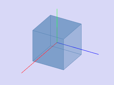
Любое вращение в трехмерном пространстве может быть представлено как композиция поворотов вокруг трех ортогональных осей (например, вокруг осей декартовых координат). Этой композиции соответствует матрица, равная произведению соответствующих трех матриц поворота.
Матрицами вращения вокруг оси декартовой системы координат на угол α в трёхмерном пространстве являются:
Вращение вокруг оси x:
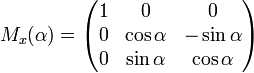
Вращение вокруг оси y:
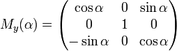
Вращение вокруг оси z:

После преобразований мы получаем формулы:
По оси Х
x’=x;
y’:=y*cos(L)+z*sin(L) ;
z’:=-y*sin(L)+z*cos(L) ;
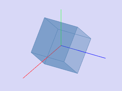
По оси Y
x’=x*cos(L)+z*sin(L);
y’=y;
z’=-x*sin(L)+z*cos(L);
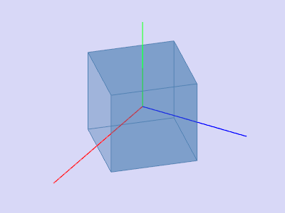
По оси Z
x’=x*cos(L)-y*sin(L);
y’=-x*sin(L)+y*cos(L);
z’=z;
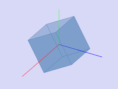
Все три поворота делаются независимо друг от друга, т.е. если надо повернуть вокруг осей Ox и Oy, вначале делается поворот вокруг оси Ox, потом применительно к полученной точки делается поворот вокруг оси Oy.
Положительным углам при этом соответствует вращение вектора против часовой стрелки в правой системе координат, и по часовой стрелке в левой системе координат, если смотреть против направления соответствующей оси. Правая система координат связана с выбором правого базиса (см. правило буравчика).