Формула для расчета медианы в статистике
Медианная формула в статистике относится к формуле, используемой для определения среднего числа в заданном наборе данных, расположенном в порядке возрастания. Согласно подсчету формулы количество элементов в наборе данных добавляется к единице. Таким образом, результаты будут разделены на два, чтобы получить место срединного значения, т. е. число, помещенное в идентифицированную позицию, будет средним значением.
Это инструмент для измерения центра набора числовых данных. Он суммирует большие объемы данных в одно значение. Его можно определить как среднее число группы чисел, отсортированных в порядке возрастания. Другими словами, медиана — это число, над которым и под ним будет одинаковое количество чисел в указанной группе данных. Это широко используемая мера наборов данных в статистике. В статистике статистика — это наука, стоящая за выявлением, сбором, организацией и обобщением, анализом, интерпретацией и, наконец, представлением таких данных, как качественных, так и количественных, что помогает принимать более эффективные и эффективные решения с уместностью. читать дальше и теория вероятностей.
Медиана = {(n+1)/2}-й

Где «n» — количество элементов в наборе данных, а «th» означает (n)-е число.
Оглавление
- Формула для расчета медианы в статистике
- Расчет медианы (шаг за шагом)
- Примеры формулы медианы в статистике
- Пример №1
- Пример #2
- Пример №3
- Актуальность и использование
- Медианная формула в статистике (с шаблоном Excel)
- Рекомендуемые статьи
Расчет медианы (шаг за шагом)
Выполните следующие шаги:
- Во-первых, отсортируйте числа в порядке возрастания. Числа располагаются по возрастанию при расположении от наименьшего к наибольшему порядку в этой группе.
- Метод нахождения медианы нечетных/четных чисел в группе приведен ниже.
- Если количество элементов в группе нечетное – Найдите {(n+1)/2}-й член. Значение, соответствующее этому термину, является медианой.
- Если количество элементов в группе четное — Найдите {(n+1)/2}-й член в этой группе. Средняя точка между числами по обе стороны от срединной позиции. Например, если имеется восемь наблюдений, медиана равна (8+1)/2-й позиции, то есть можно вычислить 4,5-ю медиану, добавив 4-й и 5-й члены в этой группе, которая затем делится на 2.
Примеры формулы медианы в статистике
.free_excel_div{фон:#d9d9d9;размер шрифта:16px;радиус границы:7px;позиция:относительная;margin:30px;padding:25px 25px 25px 45px}.free_excel_div:before{content:»»;фон:url(центр центр без повтора #207245;ширина:70px;высота:70px;позиция:абсолютная;верх:50%;margin-top:-35px;слева:-35px;граница:5px сплошная #fff;граница-радиус:50%} Вы можете скачать этот шаблон Excel с медианной формулой здесь – Шаблон медианной формулы Excel
Пример №1
Список чисел: 4, 10, 7, 15, 2. Вычислить медиану.
Решение: Расположим числа в порядке возрастания.
В порядке возрастания числа: 2,4,7,10,15.
Всего 5 номеров. Медиана равна (n+1)/2-му значению. Таким образом, медиана равна (5+1)/2-му значению.
Медиана = 3-е значение.
3-е значение в списке 2, 4, 710, 15 равно 7.
Таким образом, медиана равна 7.
Пример #2
Предположим, в организации 10 сотрудников, включая генерального директора. Генеральный директор Адам Смит считает, что зарплата сотрудников высока. Следовательно, он хочет оценить зарплату, получаемую группой, и, следовательно, принимать решения.
Ниже указана заработная плата сотрудников фирмы. Рассчитайте среднюю заработную плату. Заработная плата составляет 5 000 долларов, 6 000 долларов, 4 000 долларов, 7 000 долларов, 8 000 долларов, 7 500 долларов, 10 000 долларов, 12 000 долларов, 4 500 долларов, 10 00 000 долларов.
Решение:
Сначала расположим оклады в порядке возрастания. Заработная плата в порядке возрастания:
4000 долларов, 4500 долларов, 5000 долларов, 6000 долларов, 7000 долларов, 7500 долларов, 8000 долларов, 10000 долларов, 12000 долларов, 1000000 долларов

Таким образом, расчет медианы будет следующим:
Поскольку элементов 10, медиана равна (10+1)/2-му элементу. Медиана = 5,5-й пункт.
Таким образом, медиана — это среднее значение 5-го и 6-го пунктов. Например, 5-й и 6-й предметы стоят 7000 и 7500 долларов.
= (7000 долл. США + 7500 долл. США)/2 = 7250 долл. США.
Таким образом, средняя заработная плата 10 сотрудников составляет 7250 долларов.
Пример №3
Джеффу Смиту, генеральному директору производственной организации, необходимо заменить семь машин новыми. Однако он обеспокоен понесенными затратами и звонит финансовому директору фирмы, чтобы тот помог ему рассчитать медианную стоимость семи новых машин.
Финансовый менеджер предположил, что можно покупать новые машины, если средняя цена машин ниже 85 000 долларов. Затраты следующие: 75 000 долларов, 82 500 долларов, 60 000 долларов, 50 000 долларов, 1 00 000 долларов, 70 000 долларов, 90 000 долларов. Рассчитайте среднюю стоимость машин. Затраты следующие: 75 000 долларов, 82 500 долларов, 60 000 долларов, 50 000 долларов, 1 00 000 долларов, 70 000 долларов, 90 000 долларов.
Решение:
Расположите затраты в порядке возрастания: 50 000 долларов, 60 000 долларов, 70 000 долларов, 75 000 долларов, 82 500 долларов, 90 000 долларов, 1 00 000 долларов.
Таким образом, расчет медианы будет следующим:
Поскольку элементов 7, медиана равна (7+1)/2-й элемент, т. е. 4-й элемент. Следовательно, 4-й предмет стоит 75 000 долларов.
Поскольку медиана ниже 85 000 долларов, можно купить новые машины.
Актуальность и использование
Основное преимущество медианы перед средними заключается в том, что на нее не оказывают чрезмерного влияния крайние значения, которые могут быть очень высокими и очень низкими. Таким образом, это дает человеку лучшее представление о репрезентативной ценности. Например, если вес 5 человек в кг равен 50, 55, 55, 60 и 150. Среднее значение равно (50+55+55+60+150)/5 = 74 кг. Однако 74 кг не является истинным репрезентативным значением, поскольку большинство весов находится в диапазоне от 50 до 60. Вычислим медиану в таком случае. Это будет (5+1)/2-й член = 3-й член. Третий член — 55 кг, что является медианой. Поскольку большинство данных находится в диапазоне от 50 до 60, 55 кг являются истинным репрезентативным значением данных.
Мы должны быть осторожны в интерпретации того, что означает медиана. Например, когда мы говорим, что средний вес составляет 55 кг, не все люди весят 55 кг. Кто-то может весить больше, а кто-то меньше. Однако 55 кг – это хороший показатель веса 5 человек.
В реальном мире, чтобы понять наборы данных, такие как доход домохозяйства или активы домохозяйства, которые сильно различаются, среднее значение может быть искажено небольшим количеством очень больших значений или малых значений. Таким образом, медиана используется, чтобы предположить, каким должно быть типичное значение.
Медианная формула в статистике (с шаблоном Excel)
Билл — владелец обувного магазина. Он хочет знать, какой размер обуви ему следует заказать. Он спрашивает 9 покупателей, какой у них размер обуви. Результатами являются 7, 6, 8, 8, 10, 6, 7, 9 и 6. Вычислите медиану, чтобы помочь Биллу принять решение о заказе.
Решение: Сначала мы должны расположить размеры обуви в порядке возрастания.
Это: 6, 6, 6, 7, 7, 8, 8, 9, 10
Ниже приведены данные для расчета медианы обувного магазина.

Поэтому вычисление медианы в excelMedian In ExcelMEDIAN в Excel дает медиану заданного набора чисел. МЕДИАНА Определяет положение центра группы чисел в статистическом распределении. Подробнее будет следующим:

В Excel можно использовать встроенную формулу для медианы, чтобы вычислить медиану группы чисел. Выберите пустую ячейку и введите это = МЕДИАНА (B2: B10) (B2: B10 указывает диапазон, из которого вы хотите вычислить медиану).
Медиана обувного магазина будет –

Рекомендуемые статьи
Эта статья была руководством по медианной формуле в статистике. Здесь мы обсуждаем расчет медианы с использованием ее формулы и практических примеров в Excel и загружаемого шаблона Excel. Вы можете узнать больше об Excel из следующих статей: –
- ФормулаФормулаНормальное распределение – это симметричное распределение, т.е. положительные и отрицательные значения распределения можно разделить на равные половины, и поэтому среднее значение, медиана и мода будут равны. У него два хвоста, один известен как правый хвост, а другой известен как левый хвост. Узнайте больше о нормальном распределении нормального распределения. на равные половины и, следовательно, среднее значение, медиана и мода будут равны. У него два хвоста, один известен как правый хвост, а другой известен как левый хвост.Подробнее
- Вычислить стандартное нормальное распределениеВычислить стандартное нормальное распределениеСтандартное нормальное распределение — это симметричное распределение вероятностей относительно среднего или среднего значения, показывающее, что данные, близкие к среднему или среднему, встречаются чаще, чем данные, далекие от среднего или нормы. Таким образом, оценка называется «Z-оценка».Подробнее
- Формула МЕДИАНА в ExcelФормула МЕДИАНА в Excel Функция МЕДИАНА в Excel дает медиану заданного набора чисел. МЕДИАНА Определяет расположение центра группы чисел в статистическом распределении.Подробнее
- Вычислить среднее значение населенияВычислить среднее значение населенияСреднее значение населения представляет собой среднее значение всех значений в данной совокупности и рассчитывается как сумма всех значений в совокупности, обозначаемая суммой X, деленная на количество значений в совокупности, которое обозначается N. читать далее
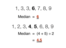
Finding the median in sets of data with an odd and even number of values
In statistics and probability theory, the median is the value separating the higher half from the lower half of a data sample, a population, or a probability distribution. For a data set, it may be thought of as «the middle» value. The basic feature of the median in describing data compared to the mean (often simply described as the «average») is that it is not skewed by a small proportion of extremely large or small values, and therefore provides a better representation of the center. Median income, for example, may be a better way to describe center of the income distribution because increases in the largest incomes alone have no effect on median. For this reason, the median is of central importance in robust statistics.
Finite data set of numbers[edit]
The median of a finite list of numbers is the «middle» number, when those numbers are listed in order from smallest to greatest.
If the data set has an odd number of observations, the middle one is selected. For example, the following list of seven numbers,
- 1, 3, 3, 6, 7, 8, 9
has the median of 6, which is the fourth value.
If the data set has an even number of observations, there is no distinct middle value and the median is usually defined to be the arithmetic mean of the two middle values.[1][2] For example, this data set of 8 numbers
- 1, 2, 3, 4, 5, 6, 8, 9
has a median value of 4.5, that is  . (In more technical terms, this interprets the median as the fully trimmed mid-range).
In general, with this convention, the median can be defined as follows: For a data set  of
of  elements, ordered from smallest to greatest,
- if
 is odd,
 - if is even,


| Type | Description | Example | Result |
|---|---|---|---|
| Midrange | Midway point between the minimum and the maximum of a data set | 1, 2, 2, 3, 4, 7, 9 | 5 |
| Arithmetic mean | Sum of values of a data set divided by number of values: 
|
(1 + 2 + 2 + 3 + 4 + 7 + 9) / 7 | 4 |
| Median | Middle value separating the greater and lesser halves of a data set | 1, 2, 2, 3, 4, 7, 9 | 3 |
| Mode | Most frequent value in a data set | 1, 2, 2, 3, 4, 7, 9 | 2 |
Formal definition[edit]
Formally, a median of a population is any value such that at least half of the population is less than or equal to the proposed median and at least half is greater than or equal to the proposed median. As seen above, medians may not be unique. If each set contains more than half the population, then some of the population is exactly equal to the unique median.
The median is well-defined for any ordered (one-dimensional) data, and is independent of any distance metric. The median can thus be applied to classes which are ranked but not numerical (e.g. working out a median grade when students are graded from A to F), although the result might be halfway between classes if there is an even number of cases.
A geometric median, on the other hand, is defined in any number of dimensions. A related concept, in which the outcome is forced to correspond to a member of the sample, is the medoid.
There is no widely accepted standard notation for the median, but some authors represent the median of a variable x either as x͂ or as μ1/2[1] sometimes also M.[3][4] In any of these cases, the use of these or other symbols for the median needs to be explicitly defined when they are introduced.
The median is a special case of other ways of summarizing the typical values associated with a statistical distribution: it is the 2nd quartile, 5th decile, and 50th percentile.
Uses[edit]
The median can be used as a measure of location when one attaches reduced importance to extreme values, typically because a distribution is skewed, extreme values are not known, or outliers are untrustworthy, i.e., may be measurement/transcription errors.
For example, consider the multiset
- 1, 2, 2, 2, 3, 14.
The median is 2 in this case, as is the mode, and it might be seen as a better indication of the center than the arithmetic mean of 4, which is larger than all but one of the values. However, the widely cited empirical relationship that the mean is shifted «further into the tail» of a distribution than the median is not generally true. At most, one can say that the two statistics cannot be «too far» apart; see § Inequality relating means and medians below.[5]
As a median is based on the middle data in a set, it is not necessary to know the value of extreme results in order to calculate it. For example, in a psychology test investigating the time needed to solve a problem, if a small number of people failed to solve the problem at all in the given time a median can still be calculated.[6]
Because the median is simple to understand and easy to calculate, while also a robust approximation to the mean, the median is a popular summary statistic in descriptive statistics. In this context, there are several choices for a measure of variability: the range, the interquartile range, the mean absolute deviation, and the median absolute deviation.
For practical purposes, different measures of location and dispersion are often compared on the basis of how well the corresponding population values can be estimated from a sample of data. The median, estimated using the sample median, has good properties in this regard. While it is not usually optimal if a given population distribution is assumed, its properties are always reasonably good. For example, a comparison of the efficiency of candidate estimators shows that the sample mean is more statistically efficient when—and only when— data is uncontaminated by data from heavy-tailed distributions or from mixtures of distributions.[citation needed] Even then, the median has a 64% efficiency compared to the minimum-variance mean (for large normal samples), which is to say the variance of the median will be ~50% greater than the variance of the mean.[7][8]
Probability distributions[edit]

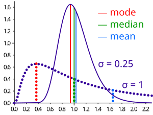
Geometric visualization of the mode, median and mean of an arbitrary probability density function[9]
For any real-valued probability distribution with cumulative distribution function F, a median is defined as any real number m that satisfies the inequalities
![{displaystyle int _{(-infty ,m]}dF(x)geq {frac {1}{2}}{text{ and }}int _{[m,infty )}dF(x)geq {frac {1}{2}}.}](https://wikimedia.org/api/rest_v1/media/math/render/svg/6f38cd2176b48f55c51f4ce62dd514aac773273f)
An equivalent phrasing uses a random variable X distributed according to F:

Note that this definition does not require X to have an absolutely continuous distribution (which has a probability density function f), nor does it require a discrete one. In the former case, the inequalities can be upgraded to equality: a median satisfies

Any probability distribution on R has at least one median, but in pathological cases there may be more than one median: if F is constant 1/2 on an interval (so that f=0 there), then any value of that interval is a median.
Medians of particular distributions[edit]
The medians of certain types of distributions can be easily calculated from their parameters; furthermore, they exist even for some distributions lacking a well-defined mean, such as the Cauchy distribution:
- The median of a symmetric unimodal distribution coincides with the mode.
- The median of a symmetric distribution which possesses a mean μ also takes the value μ.
- The median of a normal distribution with mean μ and variance σ2 is μ. In fact, for a normal distribution, mean = median = mode.
- The median of a uniform distribution in the interval [a, b] is (a + b) / 2, which is also the mean.
- The median of a Cauchy distribution with location parameter x0 and scale parameter y is x0, the location parameter.
- The median of a power law distribution x−a, with exponent a > 1 is 21/(a − 1)xmin, where xmin is the minimum value for which the power law holds[10]
- The median of an exponential distribution with rate parameter λ is the natural logarithm of 2 divided by the rate parameter: λ−1ln 2.
- The median of a Weibull distribution with shape parameter k and scale parameter λ is λ(ln 2)1/k.
Properties[edit]
Optimality property[edit]
The mean absolute error of a real variable c with respect to the random variable X is

Provided that the probability distribution of X is such that the above expectation exists, then m is a median of X if and only if m is a minimizer of the mean absolute error with respect to X.[11] In particular, if m is a sample median, then it minimizes the arithmetic mean of the absolute deviations.[12] Note, however, that in cases where the sample contains an even number of elements, this minimizer is not unique.
More generally, a median is defined as a minimum of

as discussed below in the section on multivariate medians (specifically, the spatial median).
This optimization-based definition of the median is useful in statistical data-analysis, for example, in k-medians clustering.
Inequality relating means and medians[edit]
If the distribution has finite variance, then the distance between the median  and the mean
  is bounded by one standard deviation.
This bound was proved by Book and Sher in 1979 for discrete samples,[13] and more generally by Page and Murty in 1982.[14] In a comment on a subsequent proof by O’Cinneide,[15] Mallows in 1991 presented a compact proof that uses Jensen’s inequality twice,[16] as follows. Using |·| for the absolute value, we have

The first and third inequalities come from Jensen’s inequality applied to the absolute-value function and the square function, which are each convex. The second inequality comes from the fact that a median minimizes the absolute deviation function  .
.
Mallows’s proof can be generalized to obtain a multivariate version of the inequality[17] simply by replacing the absolute value with a norm:

where m is a spatial median, that is, a minimizer of the function  The spatial median is unique when the data-set’s dimension is two or more.[18][19]
An alternative proof uses the one-sided Chebyshev inequality; it appears in an inequality on location and scale parameters. This formula also follows directly from Cantelli’s inequality.[20]
Unimodal distributions[edit]
For the case of unimodal distributions, one can achieve a sharper bound on the distance between the median and the mean:
- .[21]

A similar relation holds between the median and the mode:

Jensen’s inequality for medians[edit]
Jensen’s inequality states that for any random variable X with a finite expectation E[X] and for any convex function f
![{displaystyle f[E(x)]leq E[f(x)]}](https://wikimedia.org/api/rest_v1/media/math/render/svg/1874d0eeb97b95fcab3c70f25df212e2cb4af2d2)
This inequality generalizes to the median as well. We say a function f: R → R is a C function if, for any t,
![{displaystyle f^{-1}left(,(-infty ,t],right)={xin mathbb {R} mid f(x)leq t}}](https://wikimedia.org/api/rest_v1/media/math/render/svg/0bb6a4a02d8480c441a0f73bea93cc4fffb9b08d)
is a closed interval (allowing the degenerate cases of a single point or an empty set). Every convex function is a C function, but the reverse does not hold. If f is a C function, then
![{displaystyle f(operatorname {Median} [X])leq operatorname {Median} [f(X)]}](https://wikimedia.org/api/rest_v1/media/math/render/svg/71d1c1e4434b41fe5617b85c49b2e9d308c8a1a3)
If the medians are not unique, the statement holds for the corresponding suprema.[22]
Medians for samples[edit]
This section discusses the theory of estimating a population median from a sample. To calculate the median of a sample «by hand,» see § Finite data set of numbers above.
The sample median[edit]
Efficient computation of the sample median[edit]
Even though comparison-sorting n items requires Ω(n log n) operations, selection algorithms can compute the kth-smallest of n items with only Θ(n) operations. This includes the median, which is the n/2th order statistic (or for an even number of samples, the arithmetic mean of the two middle order statistics).[23]
Selection algorithms still have the downside of requiring Ω(n) memory, that is, they need to have the full sample (or a linear-sized portion of it) in memory. Because this, as well as the linear time requirement, can be prohibitive, several estimation procedures for the median have been developed. A simple one is the median of three rule, which estimates the median as the median of a three-element subsample; this is commonly used as a subroutine in the quicksort sorting algorithm, which uses an estimate of its input’s median. A more robust estimator is Tukey’s ninther, which is the median of three rule applied with limited recursion:[24] if A is the sample laid out as an array, and
- med3(A) = median(A[1], A[n/2], A[n]),
then
- ninther(A) = med3(med3(A[1 … 1/3n]), med3(A[1/3n … 2/3n]), med3(A[2/3n … n]))
The remedian is an estimator for the median that requires linear time but sub-linear memory, operating in a single pass over the sample.[25]
Sampling distribution[edit]
The distributions of both the sample mean and the sample median were determined by Laplace.[26] The distribution of the sample median from a population with a density function  is asymptotically normal with mean
  and variance[27]

where  is the median of and is the sample size:

A modern proof follows below. Laplace’s result is now understood as a special case of the asymptotic distribution of arbitrary quantiles.
For normal samples, the density is  , thus for large samples the variance of the median equals
  [7] (See also section #Efficiency below.)
Derivation of the asymptotic distribution[edit]
We take the sample size to be an odd number  and assume our variable continuous; the formula for the case of discrete variables is given below in § Empirical local density. The sample can be summarized as «below median», «at median», and «above median», which corresponds to a trinomial distribution with probabilities
  ,
,  and
and  . For a continuous variable, the probability of multiple sample values being exactly equal to the median is 0, so one can calculate the density of at the point
  directly from the trinomial distribution:
- .
![{displaystyle Pr[operatorname {Median} =v],dv={frac {(2n+1)!}{n!n!}}F(v)^{n}(1-F(v))^{n}f(v),dv}](https://wikimedia.org/api/rest_v1/media/math/render/svg/b99f214189b2882487bfbae7997046efa4a88cc4)
Now we introduce the beta function. For integer arguments  and
and  , this can be expressed as
  . Also, recall that
  . Using these relationships and setting both and equal to
  allows the last expression to be written as

Hence the density function of the median is a symmetric beta distribution pushed forward by  . Its mean, as we would expect, is 0.5 and its variance is
  . By the chain rule, the corresponding variance of the sample median is
- .

The additional 2 is negligible in the limit.
Empirical local density[edit]
In practice, the functions  and are often not known or assumed. However, they can be estimated from an observed frequency distribution. In this section, we give an example. Consider the following table, representing a sample of 3,800 (discrete-valued) observations:
| v | 0 | 0.5 | 1 | 1.5 | 2 | 2.5 | 3 | 3.5 | 4 | 4.5 | 5 |
|---|---|---|---|---|---|---|---|---|---|---|---|
| f(v) | 0.000 | 0.008 | 0.010 | 0.013 | 0.083 | 0.108 | 0.328 | 0.220 | 0.202 | 0.023 | 0.005 |
| F(v) | 0.000 | 0.008 | 0.018 | 0.031 | 0.114 | 0.222 | 0.550 | 0.770 | 0.972 | 0.995 | 1.000 |
Because the observations are discrete-valued, constructing the exact distribution of the median is not an immediate translation of the above expression for  ; one may (and typically does) have multiple instances of the median in one’s sample. So we must sum over all these possibilities:

Here, i is the number of points strictly less than the median and k the number strictly greater.
Using these preliminaries, it is possible to investigate the effect of sample size on the standard errors of the mean and median. The observed mean is 3.16, the observed raw median is 3 and the observed interpolated median is 3.174. The following table gives some comparison statistics.
|
Sample size Statistic |
3 | 9 | 15 | 21 |
|---|---|---|---|---|
| Expected value of median | 3.198 | 3.191 | 3.174 | 3.161 |
| Standard error of median (above formula) | 0.482 | 0.305 | 0.257 | 0.239 |
| Standard error of median (asymptotic approximation) | 0.879 | 0.508 | 0.393 | 0.332 |
| Standard error of mean | 0.421 | 0.243 | 0.188 | 0.159 |
The expected value of the median falls slightly as sample size increases while, as would be expected, the standard errors of both the median and the mean are proportionate to the inverse square root of the sample size. The asymptotic approximation errs on the side of caution by overestimating the standard error.
Estimation of variance from sample data[edit]
The value of  —the asymptotic value of
  where
where  is the population median—has been studied by several authors. The standard «delete one» jackknife method produces inconsistent results.[28] An alternative—the «delete k» method—where
  grows with the sample size has been shown to be asymptotically consistent.[29] This method may be computationally expensive for large data sets. A bootstrap estimate is known to be consistent,[30] but converges very slowly (order of
  ).[31] Other methods have been proposed but their behavior may differ between large and small samples.[32]
Efficiency[edit]
The efficiency of the sample median, measured as the ratio of the variance of the mean to the variance of the median, depends on the sample size and on the underlying population distribution. For a sample of size from the normal distribution, the efficiency for large N is

The efficiency tends to  as
as  tends to infinity.
In other words, the relative variance of the median will be  , or 57% greater than the variance of the mean – the relative standard error of the median will be
  , or 25% greater than the standard error of the mean,
  (see also section #Sampling distribution above.).[33]
Other estimators[edit]
For univariate distributions that are symmetric about one median, the Hodges–Lehmann estimator is a robust and highly efficient estimator of the population median.[34]
If data is represented by a statistical model specifying a particular family of probability distributions, then estimates of the median can be obtained by fitting that family of probability distributions to the data and calculating the theoretical median of the fitted distribution.[citation needed] Pareto interpolation is an application of this when the population is assumed to have a Pareto distribution.
Multivariate median[edit]
Previously, this article discussed the univariate median, when the sample or population had one-dimension. When the dimension is two or higher, there are multiple concepts that extend the definition of the univariate median; each such multivariate median agrees with the univariate median when the dimension is exactly one.[34][35][36][37]
Marginal median[edit]
The marginal median is defined for vectors defined with respect to a fixed set of coordinates. A marginal median is defined to be the vector whose components are univariate medians. The marginal median is easy to compute, and its properties were studied by Puri and Sen.[34][38]
Geometric median[edit]
The geometric median of a discrete set of sample points  in a Euclidean space is the[a] point minimizing the sum of distances to the sample points.

In contrast to the marginal median, the geometric median is equivariant with respect to Euclidean similarity transformations such as translations and rotations.
Median in all directions[edit]
If the marginal medians for all coordinate systems coincide, then their common location may be termed the «median in all directions».[40] This concept is relevant to voting theory on account of the median voter theorem. When it exists, the median in all directions coincides with the geometric median (at least for discrete distributions).
Centerpoint[edit]
An alternative generalization of the median in higher dimensions is the centerpoint.
[edit]
Interpolated median[edit]
When dealing with a discrete variable, it is sometimes useful to regard the observed values as being midpoints of underlying continuous intervals. An example of this is a Likert scale, on which opinions or preferences are expressed on a scale with a set number of possible responses. If the scale consists of the positive integers, an observation of 3 might be regarded as representing the interval from 2.50 to 3.50. It is possible to estimate the median of the underlying variable. If, say, 22% of the observations are of value 2 or below and 55.0% are of 3 or below (so 33% have the value 3), then the median is 3 since the median is the smallest value of for which  is greater than a half. But the interpolated median is somewhere between 2.50 and 3.50. First we add half of the interval width
  to the median to get the upper bound of the median interval. Then we subtract that proportion of the interval width which equals the proportion of the 33% which lies above the 50% mark. In other words, we split up the interval width pro rata to the numbers of observations. In this case, the 33% is split into 28% below the median and 5% above it so we subtract 5/33 of the interval width from the upper bound of 3.50 to give an interpolated median of 3.35. More formally, if the values are known, the interpolated median can be calculated from
![{displaystyle m_{text{int}}=m+wleft[{frac {1}{2}}-{frac {F(m)-{frac {1}{2}}}{f(m)}}right].}](https://wikimedia.org/api/rest_v1/media/math/render/svg/5e823608d9eba650d4796825d3043ef41d06370e)
Alternatively, if in an observed sample there are scores above the median category,  scores in it and
  scores below it then the interpolated median is given by
![{displaystyle m_{text{int}}=m+{frac {w}{2}}left[{frac {k-i}{j}}right].}](https://wikimedia.org/api/rest_v1/media/math/render/svg/8519008345d5bd2863ff18203d1b6144f851ae95)
Pseudo-median[edit]
For univariate distributions that are symmetric about one median, the Hodges–Lehmann estimator is a robust and highly efficient estimator of the population median; for non-symmetric distributions, the Hodges–Lehmann estimator is a robust and highly efficient estimator of the population pseudo-median, which is the median of a symmetrized distribution and which is close to the population median.[41] The Hodges–Lehmann estimator has been generalized to multivariate distributions.[42]
Variants of regression[edit]
The Theil–Sen estimator is a method for robust linear regression based on finding medians of slopes.[43]
Median filter[edit]
The median filter is an important tool of image processing, that can effectively remove any salt and pepper noise from grayscale images.
Cluster analysis[edit]
In cluster analysis, the k-medians clustering algorithm provides a way of defining clusters, in which the criterion of maximising the distance between cluster-means that is used in k-means clustering, is replaced by maximising the distance between cluster-medians.
Median–median line[edit]
This is a method of robust regression. The idea dates back to Wald in 1940 who suggested dividing a set of bivariate data into two halves depending on the value of the independent parameter : a left half with values less than the median and a right half with values greater than the median.[44] He suggested taking the means of the dependent  and independent variables of the left and the right halves and estimating the slope of the line joining these two points. The line could then be adjusted to fit the majority of the points in the data set.
Nair and Shrivastava in 1942 suggested a similar idea but instead advocated dividing the sample into three equal parts before calculating the means of the subsamples.[45] Brown and Mood in 1951 proposed the idea of using the medians of two subsamples rather the means.[46] Tukey combined these ideas and recommended dividing the sample into three equal size subsamples and estimating the line based on the medians of the subsamples.[47]
Median-unbiased estimators[edit]
Any mean-unbiased estimator minimizes the risk (expected loss) with respect to the squared-error loss function, as observed by Gauss. A median-unbiased estimator minimizes the risk with respect to the absolute-deviation loss function, as observed by Laplace. Other loss functions are used in statistical theory, particularly in robust statistics.
The theory of median-unbiased estimators was revived by George W. Brown in 1947:[48]
An estimate of a one-dimensional parameter θ will be said to be median-unbiased if, for fixed θ, the median of the distribution of the estimate is at the value θ; i.e., the estimate underestimates just as often as it overestimates. This requirement seems for most purposes to accomplish as much as the mean-unbiased requirement and has the additional property that it is invariant under one-to-one transformation.
— page 584
Further properties of median-unbiased estimators have been reported.[49][50][51][52] Median-unbiased estimators are invariant under one-to-one transformations.
There are methods of constructing median-unbiased estimators that are optimal (in a sense analogous to the minimum-variance property for mean-unbiased estimators). Such constructions exist for probability distributions having monotone likelihood-functions.[53][54] One such procedure is an analogue of the Rao–Blackwell procedure for mean-unbiased estimators: The procedure holds for a smaller class of probability distributions than does the Rao—Blackwell procedure but for a larger class of loss functions.[55]
History[edit]
Scientific researchers in the ancient near east appear not to have used summary statistics altogether, instead choosing values that offered maximal consistency with a broader theory that integrated a wide variety of phenomena.[56] Within the Mediterranean (and, later, European) scholarly community, statistics like the mean are fundamentally a medieval and early modern development. (The history of the median outside Europe and its predecessors remains relatively unstudied.)
The idea of the median appeared in the 6th century in the Talmud, in order to fairly analyze divergent appraisals.[57][58] However, the concept did not spread to the broader scientific community.
Instead, the closest ancestor of the modern median is the mid-range, invented by Al-Biruni.[59]: 31 [60] Transmission of Al-Biruni’s work to later scholars is unclear. Al-Biruni applied his technique to assaying metals, but, after he published his work, most assayers still adopted the most unfavorable value from their results, lest they appear to cheat.[59]: 35–8 However, increased navigation at sea during the Age of Discovery meant that ship’s navigators increasingly had to attempt to determine latitude in unfavorable weather against hostile shores, leading to renewed interest in summary statistics. Whether rediscovered or independently invented, the mid-range is recommended to nautical navigators in Harriot’s «Instructions for Raleigh’s Voyage to Guiana, 1595».[59]: 45–8
The idea of the median may have first appeared in Edward Wright’s 1599 book Certaine Errors in Navigation on a section about compass navigation. Wright was reluctant to discard measured values, and may have felt that the median — incorporating a greater proportion of the dataset than the mid-range — was more likely to be correct. However, Wright did not give examples of his technique’s use, making it hard to verify that he described the modern notion of median.[56][60][b] The median (in the context of probability) certainly appeared in the correspondence of Christiaan Huygens, but as an example of a statistic that was inappropriate for actuarial practice.[56]
The earliest recommendation of the median dates to 1757, when Roger Joseph Boscovich developed a regression method based on the L1 norm and therefore implicitly on the median.[56][61] In 1774, Laplace made this desire explicit: he suggested the median be used as the standard estimator of the value of a posterior PDF. The specific criterion was to minimize the expected magnitude of the error;  where
where  is the estimate and is the true value. To this end, Laplace determined the distributions of both the sample mean and the sample median in the early 1800s.[26][62] However, a decade later, Gauss and Legendre developed the least squares method, which minimizes
  to obtain the mean. Within the context of regression, Gauss and Legendre’s innovation offers vastly easier computation. Consequently, Laplaces’ proposal was generally rejected until the rise of computing devices 150 years later (and is still a relatively uncommon algorithm).[63]
Antoine Augustin Cournot in 1843 was the first[64] to use the term median (valeur médiane) for the value that divides a probability distribution into two equal halves. Gustav Theodor Fechner used the median (Centralwerth) in sociological and psychological phenomena.[65] It had earlier been used only in astronomy and related fields. Gustav Fechner popularized the median into the formal analysis of data, although it had been used previously by Laplace,[65] and the median appeared in a textbook by F. Y. Edgeworth.[66] Francis Galton used the English term median in 1881,[67][68] having earlier used the terms middle-most value in 1869, and the medium in 1880.[69][70]
Statisticians encouraged the use of medians intensely throughout the 19th century for its intuitive clarity and ease of manual computation. However, the notion of median does not lend itself to the theory of higher moments as well as the arithmetic mean does, and is much harder to compute by computer. As a result, the median was steadily supplanted as a notion of generic average by the arithmetic mean during the 20th century.[56][60]
See also[edit]
- Absolute deviation
- Bias of an estimator
- Central tendency
- Concentration of measure for Lipschitz functions
- Median graph
- Median of medians – Algorithm to calculate the approximate median in linear time
- Median search
- Median slope
- Median voter theory
- Medoids – Generalization of the median in higher dimensions
Notes[edit]
- ^ The geometric median is unique unless the sample is collinear.[39]
- ^ Subsequent scholars appear to concur with Eisenhart that Boroughs’ 1580 figures, while suggestive of the median, in fact describe an arithmetic mean.;[59]: 62–3 Boroughs is mentioned in no other work.
References[edit]
- ^ a b Weisstein, Eric W. «Statistical Median». MathWorld.
- ^ Simon, Laura J.; «Descriptive statistics» Archived 2010-07-30 at the Wayback Machine, Statistical Education Resource Kit, Pennsylvania State Department of Statistics
- ^ David J. Sheskin (27 August 2003). Handbook of Parametric and Nonparametric Statistical Procedures (Third ed.). CRC Press. pp. 7–. ISBN 978-1-4200-3626-8. Retrieved 25 February 2013.
- ^ Derek Bissell (1994). Statistical Methods for Spc and Tqm. CRC Press. pp. 26–. ISBN 978-0-412-39440-9. Retrieved 25 February 2013.
- ^ Paul T. von Hippel (2005). «Mean, Median, and Skew: Correcting a Textbook Rule». Journal of Statistics Education. 13 (2). Archived from the original on 2008-10-14. Retrieved 2015-06-18.
- ^ Robson, Colin (1994). Experiment, Design and Statistics in Psychology. Penguin. pp. 42–45. ISBN 0-14-017648-9.
- ^ a b Williams, D. (2001). Weighing the Odds. Cambridge University Press. p. 165. ISBN 052100618X.
- ^ Maindonald, John; Braun, W. John (2010-05-06). Data Analysis and Graphics Using R: An Example-Based Approach. Cambridge University Press. p. 104. ISBN 978-1-139-48667-5.
- ^ «AP Statistics Review — Density Curves and the Normal Distributions». Archived from the original on 8 April 2015. Retrieved 16 March 2015.
- ^ Newman, Mark EJ. «Power laws, Pareto distributions and Zipf’s law.» Contemporary physics 46.5 (2005): 323–351.
- ^ Stroock, Daniel (2011). Probability Theory. Cambridge University Press. pp. 43. ISBN 978-0-521-13250-3.
- ^ DeGroot, Morris H. (1970). Optimal Statistical Decisions. McGraw-Hill Book Co., New York-London-Sydney. p. 232. MR 0356303.
- ^ Stephen A. Book; Lawrence Sher (1979). «How close are the mean and the median?». The Two-Year College Mathematics Journal. 10 (3): 202–204. doi:10.2307/3026748. JSTOR 3026748. Retrieved 12 March 2022.
- ^ Warren Page; Vedula N. Murty (1982). «Nearness Relations Among Measures of Central Tendency and Dispersion: Part 1». The Two-Year College Mathematics Journal. 13 (5): 315–327. doi:10.1080/00494925.1982.11972639 (inactive 31 December 2022). Retrieved 12 March 2022.
{{cite journal}}: CS1 maint: DOI inactive as of December 2022 (link) - ^ O’Cinneide, Colm Art (1990). «The mean is within one standard deviation of any median». The American Statistician. 44 (4): 292–293. doi:10.1080/00031305.1990.10475743. Retrieved 12 March 2022.
- ^ Mallows, Colin (August 1991). «Another comment on O’Cinneide». The American Statistician. 45 (3): 257. doi:10.1080/00031305.1991.10475815.
- ^ Piché, Robert (2012). Random Vectors and Random Sequences. Lambert Academic Publishing. ISBN 978-3659211966.
- ^ Kemperman, Johannes H. B. (1987). Dodge, Yadolah (ed.). «The median of a finite measure on a Banach space: Statistical data analysis based on the L1-norm and related methods». Papers from the First International Conference Held at Neuchâtel, August 31–September 4, 1987. Amsterdam: North-Holland Publishing Co.: 217–230. MR 0949228.
- ^ Milasevic, Philip; Ducharme, Gilles R. (1987). «Uniqueness of the spatial median». Annals of Statistics. 15 (3): 1332–1333. doi:10.1214/aos/1176350511. MR 0902264.
- ^ K.Van Steen Notes on probability and statistics
- ^ Basu, S.; Dasgupta, A. (1997). «The Mean, Median, and Mode of Unimodal Distributions:A Characterization». Theory of Probability and Its Applications. 41 (2): 210–223. doi:10.1137/S0040585X97975447. S2CID 54593178.
- ^ Merkle, M. (2005). «Jensen’s inequality for medians». Statistics & Probability Letters. 71 (3): 277–281. doi:10.1016/j.spl.2004.11.010.
- ^ Alfred V. Aho and John E. Hopcroft and Jeffrey D. Ullman (1974). The Design and Analysis of Computer Algorithms. Reading/MA: Addison-Wesley. ISBN 0-201-00029-6. Here: Section 3.6 «Order Statistics», p.97-99, in particular Algorithm 3.6 and Theorem 3.9.
- ^ Bentley, Jon L.; McIlroy, M. Douglas (1993). «Engineering a sort function». Software: Practice and Experience. 23 (11): 1249–1265. doi:10.1002/spe.4380231105. S2CID 8822797.
- ^ Rousseeuw, Peter J.; Bassett, Gilbert W. Jr. (1990). «The remedian: a robust averaging method for large data sets» (PDF). J. Amer. Statist. Assoc. 85 (409): 97–104. doi:10.1080/01621459.1990.10475311.
- ^ a b Stigler, Stephen (December 1973). «Studies in the History of Probability and Statistics. XXXII: Laplace, Fisher and the Discovery of the Concept of Sufficiency». Biometrika. 60 (3): 439–445. doi:10.1093/biomet/60.3.439. JSTOR 2334992. MR 0326872.
- ^ Rider, Paul R. (1960). «Variance of the median of small samples from several special populations». J. Amer. Statist. Assoc. 55 (289): 148–150. doi:10.1080/01621459.1960.10482056.
- ^ Efron, B. (1982). The Jackknife, the Bootstrap and other Resampling Plans. Philadelphia: SIAM. ISBN 0898711797.
- ^ Shao, J.; Wu, C. F. (1989). «A General Theory for Jackknife Variance Estimation». Ann. Stat. 17 (3): 1176–1197. doi:10.1214/aos/1176347263. JSTOR 2241717.
- ^ Efron, B. (1979). «Bootstrap Methods: Another Look at the Jackknife». Ann. Stat. 7 (1): 1–26. doi:10.1214/aos/1176344552. JSTOR 2958830.
- ^ Hall, P.; Martin, M. A. (1988). «Exact Convergence Rate of Bootstrap Quantile Variance Estimator». Probab Theory Related Fields. 80 (2): 261–268. doi:10.1007/BF00356105. S2CID 119701556.
- ^ Jiménez-Gamero, M. D.; Munoz-García, J.; Pino-Mejías, R. (2004). «Reduced bootstrap for the median». Statistica Sinica. 14 (4): 1179–1198.
- ^ Maindonald, John; John Braun, W. (2010-05-06). Data Analysis and Graphics Using R: An Example-Based Approach. ISBN 9781139486675.
- ^ a b c Hettmansperger, Thomas P.; McKean, Joseph W. (1998). Robust nonparametric statistical methods. Kendall’s Library of Statistics. Vol. 5. London: Edward Arnold. ISBN 0-340-54937-8. MR 1604954.
- ^ Small, Christopher G. «A survey of multidimensional medians.» International Statistical Review/Revue Internationale de Statistique (1990): 263–277. doi:10.2307/1403809 JSTOR 1403809
- ^ Niinimaa, A., and H. Oja. «Multivariate median.» Encyclopedia of statistical sciences (1999).
- ^ Mosler, Karl. Multivariate Dispersion, Central Regions, and Depth: The Lift Zonoid Approach. Vol. 165. Springer Science & Business Media, 2012.
- ^ Puri, Madan L.; Sen, Pranab K.; Nonparametric Methods in Multivariate Analysis, John Wiley & Sons, New York, NY, 1971. (Reprinted by Krieger Publishing)
- ^ Vardi, Yehuda; Zhang, Cun-Hui (2000). «The multivariate L1-median and associated data depth». Proceedings of the National Academy of Sciences of the United States of America. 97 (4): 1423–1426 (electronic). Bibcode:2000PNAS…97.1423V. doi:10.1073/pnas.97.4.1423. MR 1740461. PMC 26449. PMID 10677477.
- ^ Davis, Otto A.; DeGroot, Morris H.; Hinich, Melvin J. (January 1972). «Social Preference Orderings and Majority Rule» (PDF). Econometrica. 40 (1): 147–157. doi:10.2307/1909727. JSTOR 1909727. The authors, working in a topic in which uniqueness is assumed, actually use the expression «unique median in all directions».
- ^ Pratt, William K.; Cooper, Ted J.; Kabir, Ihtisham (1985-07-11). Corbett, Francis J (ed.). «Pseudomedian Filter». Architectures and Algorithms for Digital Image Processing II. 0534: 34. Bibcode:1985SPIE..534…34P. doi:10.1117/12.946562. S2CID 173183609.
- ^ Oja, Hannu (2010). Multivariate nonparametric methods with R: An approach based on spatial signs and ranks. Lecture Notes in Statistics. Vol. 199. New York, NY: Springer. pp. xiv+232. doi:10.1007/978-1-4419-0468-3. ISBN 978-1-4419-0467-6. MR 2598854.
- ^ Wilcox, Rand R. (2001), «Theil–Sen estimator», Fundamentals of Modern Statistical Methods: Substantially Improving Power and Accuracy, Springer-Verlag, pp. 207–210, ISBN 978-0-387-95157-7.
- ^ Wald, A. (1940). «The Fitting of Straight Lines if Both Variables are Subject to Error» (PDF). Annals of Mathematical Statistics. 11 (3): 282–300. doi:10.1214/aoms/1177731868. JSTOR 2235677.
- ^ Nair, K. R.; Shrivastava, M. P. (1942). «On a Simple Method of Curve Fitting». Sankhyā: The Indian Journal of Statistics. 6 (2): 121–132. JSTOR 25047749.
- ^ Brown, G. W.; Mood, A. M. (1951). «On Median Tests for Linear Hypotheses». Proc Second Berkeley Symposium on Mathematical Statistics and Probability. Berkeley, CA: University of California Press. pp. 159–166. Zbl 0045.08606.
- ^ Tukey, J. W. (1977). Exploratory Data Analysis. Reading, MA: Addison-Wesley. ISBN 0201076160.
- ^ Brown, George W. (1947). «On Small-Sample Estimation». Annals of Mathematical Statistics. 18 (4): 582–585. doi:10.1214/aoms/1177730349. JSTOR 2236236.
- ^ Lehmann, Erich L. (1951). «A General Concept of Unbiasedness». Annals of Mathematical Statistics. 22 (4): 587–592. doi:10.1214/aoms/1177729549. JSTOR 2236928.
- ^ Birnbaum, Allan (1961). «A Unified Theory of Estimation, I». Annals of Mathematical Statistics. 32 (1): 112–135. doi:10.1214/aoms/1177705145. JSTOR 2237612.
- ^ van der Vaart, H. Robert (1961). «Some Extensions of the Idea of Bias». Annals of Mathematical Statistics. 32 (2): 436–447. doi:10.1214/aoms/1177705051. JSTOR 2237754. MR 0125674.
- ^ Pfanzagl, Johann; with the assistance of R. Hamböker (1994). Parametric Statistical Theory. Walter de Gruyter. ISBN 3-11-013863-8. MR 1291393.
- ^ Pfanzagl, Johann. «On optimal median unbiased estimators in the presence of nuisance parameters.» The Annals of Statistics (1979): 187–193.
- ^ Brown, L. D.; Cohen, Arthur; Strawderman, W. E. (1976). «A Complete Class Theorem for Strict Monotone Likelihood Ratio With Applications». Ann. Statist. 4 (4): 712–722. doi:10.1214/aos/1176343543.
- ^ Page; Brown, L. D.; Cohen, Arthur; Strawderman, W. E. (1976). «A Complete Class Theorem for Strict Monotone Likelihood Ratio With Applications». Ann. Statist. 4 (4): 712–722. doi:10.1214/aos/1176343543.
- ^ a b c d e Bakker, Arthur; Gravemeijer, Koeno P. E. (2006-06-01). «An Historical Phenomenology of Mean and Median». Educational Studies in Mathematics. 62 (2): 149–168. doi:10.1007/s10649-006-7099-8. ISSN 1573-0816. S2CID 143708116.
- ^ Adler, Dan (31 December 2014). «Talmud and Modern Economics». Jewish American and Israeli Issues. Archived from the original on 6 December 2015. Retrieved 22 February 2020.
- ^ Modern Economic Theory in the Talmud by Yisrael Aumann
- ^ a b c d Eisenhart, Churchill (24 August 1971). The Development of the Concept of the Best Mean of a Set of Measurements from Antiquity to the Present Day (PDF) (Speech). 131st Annual Meeting of the American Statistical Association. Colorado State University.
- ^ a b c «How the Average Triumphed Over the Median». Priceonomics. 5 April 2016. Retrieved 2020-02-23.
- ^ Stigler, S. M. (1986). The History of Statistics: The Measurement of Uncertainty Before 1900. Harvard University Press. ISBN 0674403401.
- ^ Laplace PS de (1818) Deuxième supplément à la Théorie Analytique des Probabilités, Paris, Courcier
- ^ Jaynes, E.T. (2007). Probability theory : the logic of science (5. print. ed.). Cambridge [u.a.]: Cambridge Univ. Press. p. 172. ISBN 978-0-521-59271-0.
- ^ Howarth, Richard (2017). Dictionary of Mathematical Geosciences: With Historical Notes. Springer. p. 374.
- ^ a b Keynes, J.M. (1921) A Treatise on Probability. Pt II Ch XVII §5 (p 201) (2006 reprint, Cosimo Classics, ISBN 9781596055308 : multiple other reprints)
- ^ Stigler, Stephen M. (2002). Statistics on the Table: The History of Statistical Concepts and Methods. Harvard University Press. pp. 105–7. ISBN 978-0-674-00979-0.
- ^ Galton F (1881) «Report of the Anthropometric Committee» pp 245–260. Report of the 51st Meeting of the British Association for the Advancement of Science
- ^ David, H. A. (1995). «First (?) Occurrence of Common Terms in Mathematical Statistics». The American Statistician. 49 (2): 121–133. doi:10.2307/2684625. ISSN 0003-1305. JSTOR 2684625.
- ^ encyclopediaofmath.org
- ^ personal.psu.edu
External links[edit]
- «Median (in statistics)», Encyclopedia of Mathematics, EMS Press, 2001 [1994]
- Median as a weighted arithmetic mean of all Sample Observations
- On-line calculator
- Calculating the median
- A problem involving the mean, the median, and the mode.
- Weisstein, Eric W. «Statistical Median». MathWorld.
- Python script for Median computations and income inequality metrics
- Fast Computation of the Median by Successive Binning
- ‘Mean, median, mode and skewness’, A tutorial devised for first-year psychology students at Oxford University, based on a worked example.
- The Complex SAT Math Problem Even the College Board Got Wrong: Andrew Daniels in Popular Mechanics
This article incorporates material from Median of a distribution on PlanetMath, which is licensed under the Creative Commons Attribution/Share-Alike License.
 В статистических исследованиях довольно широко применяются средние величины. Их нахождение позволяет выявить типичное значение признака исследуемой совокупности. Например, типичный уровень доходов покупателей или возраст большинства клиентов компании. При этом вычисление, к примеру, среднего арифметического не всегда уместно.
Представим такую ситуацию: мы опросили 10 человек на предмет их уровня доходов. У 9-х доходы оказались примерно одинаковыми и составили 10 тыс. руб. Что касается 10-ого опрошенного, то оказалось, что его доход равняется 410 тыс. руб. в месяц. Если мы вычислим простое среднее арифметическое, то типичный доход будет равняться 50 тыс. руб.! Но это явно не так. В таких ситуациях более объективную и правдоподобную картину дает вычисление моды или медианы, которые относятся к структурным средним показателям.
Понятие медианы
Медиана (Me) — значение признака в исследуемом ряду величин, которое делит этот ряд на две равные части.
То есть половина (50%) всех значений в исследуемом ряду будет меньше медианы, а другая половина — больше ее. Поэтому медиану еще называют 50-й перцентиль или квантиль 0,5.
Формула для расчета медианы
Если значений немного, то медиану можно определить «на глазок». Для этого достаточно расположить все значения в порядке возрастания и найти середину.
Если число случаев четное и в центре ряда находятся два разных числа, то медианой будет среднее между ними (даже если такого значения нет в самом ряду исследуемых случаев). Например, в ряду 1 2 3 4 5 6, медианой будет 3,5.
Для нахождения медианы в более сложных случаях (по интервальным рядам) используется специальная формула:

где: Me — медиана;
Xme — нижняя граница медианного интервала (того интервала, накопленная частота которого превышает полусумму всех частот);
ime — величина медианного интервала;
f — частота (сколько раз в ряду встречается то или иное значение);
Sme-1 — сумма частот интервалов предшествующих медианному интервалу;
fme — число значений в медианном интервале (его частота).
Пример вычисления медианы
Был проведен опрос среди покупателей с целью выяснить их типичный возраст. По результатам опроса было установлено, что: 25 покупателей имеют возраст до 20 лет; 32 покупателя — 20-40 лет; 18 покупателей — 40-60 лет; 15 покупателей — свыше 60 лет. Найдем медиану.

Сначала находим медианный интервал. Для этого вычисляем сумму частот: 25 + 32 + 18 + 15 = 90. Половина этой суммы — 45. Это соответствует возрастной группе 20-40 лет (т. к. полученная полусумма частот — 45, и накопленная частота 1-й группы меньше ее, а 3-ей — больше). Тогда нижняя граница медианного интервала — 20 (лет), а величина медианного интервала — 20 (40 лет за вычетом 20). Сумма частот интервалов предшествующих медианному интервалу — 25. Число значений в медианном интервале — 32 (количество покупателей в возрасте 20-40 лет).

Расчетное значение медианы — 32,5. Округив его, получим средний возраст покупателя — 33 года.
Область применения медианы
При вычислении типичного признака неоднородных рядов, имеющих «выбросы» — значения во много раз отличающиеся от других значений ряда.
Особенности медианы
- Медиана обладает высокой робастностью, то есть нечувствительностью к неоднородностям и ошибкам выборки;
- Сумма разностей между членами ряда выборки и медианой меньше, чем сумма этих разностей с любой другой величиной. В том числе с арифметическим средним.
Источники
- Медиана // Википедия. URL: http://ru.wikipedia.org/wiki/Медиана_(статистика) (дата обращения: 23.10.2013)
- Минашкин В. Г. и др. Курс лекций по теории статистики. – М.: МЭСИ, 2001.
© Копирование любых материалов статьи допустимо только при указании прямой индексируемой ссылки на источник: Галяутдинов Р.Р.
Нашли опечатку? Помогите сделать статью лучше! Выделите орфографическую ошибку мышью и нажмите Ctrl + Enter.
Библиографическая запись для цитирования статьи по ГОСТ Р 7.0.5-2008:
Галяутдинов Р.Р. Медиана // Сайт преподавателя экономики. [2013]. URL: https://galyautdinov.ru/post/mediana (дата обращения: 28.05.2023).
Медиана (x̃, M; Мера центральной тенденции) – это центральное значение Выборки (Sample).
В математике медиана также представляет собой тип Среднего значения (Average), который используется для нахождения «центра». Поэтому ее еще называют мерой центральной тенденции.
Нечетное количество элементов ряда
Если в ряду нечетное количество элементов, то мы сортируем значения в возрастающем или убывающем порядке, а затем выбираем центральное.
Пример. Найдем медиану следующего ряда:
4, 17, 77, 25, 22, 23, 92, 82, 40, 24, 14, 12, 67, 23, 29
Расставив эти числа по порядку, мы получим:
4, 12, 14, 17, 22, 23, 23, 24, 25, 29, 40, 67, 77, 82, 92
Всего пятнадцать элементов, то есть 8-й будет центральным. Медианное значение этого набора чисел – 24.
Четное количество элементов ряда
Если в ряду четное количество элементов, медиана рассчитывается с помощью формулы:
$$M = frac{n + 1}{2}, где$$
$$Mspace{–}space{медиана,}$$
$$nspace{–}space{количество}space{элементов}space{в}space{выборке}$$
Пример. Найдем медиану следующего ряда:
1.79, 1.61, 2.09, 1.84, 1.96, 2.11
Выполнив подстановку, мы получим:
$$M = frac{6 + 1}{2} = 3.5$$
Центральная тенденция
Помимо медианы, выделяют еще две другие меры центральной тенденции – Среднее значение (Mean) и Мода (Mode). Среднее – это частное от суммы всех Наблюдений (Observation) к их количеству. Мода – это наиболее часто повторяющееся значение выборки.
В Науке о данных (Data Science) медиана иногда используется вместо среднего значения, когда в последовательности есть выбросы, которые могут исказить среднее. Выбросы меньше влияют на медианное значение, чем на среднее. Медиана отделяет верхнюю половину выборки, генеральной совокупности или Распределения вероятностей (Probability Distribution) от нижней.

Медиана и NumPy
Медиану можно вычислить с помощью NumPy. Для начала импортируем все необходимые библиотеки:
import numpy as npСоздадим массив из 6 элементов и вызовем встроенный метод median():
a = [10, 7, 4, 3, 2, 1]
np.median(a)
NumPy определяет четность числа элементов массива (6) и применяет тот или иной метод расчета (согласно формуле):
3.5Ноутбук, не требующий дополнительной настройки на момент написания статьи, можно скачать здесь.
Фото: @garciasaldana_
Центральную тенденцию данных можно рассматривать не только, как значение с нулевым суммарным отклонением (среднее арифметическое) или максимальную частоту (мода), но и как некоторую отметку (значение в совокупности), делящую ранжированные данные (отсортированные по возрастанию или убыванию) на две равные части. Половина исходных данных меньше этой отметки, а половина – больше. Это и есть медиана.
Итак, медиана в статистике – это уровень показателя, который делит набор данных на две равные половины. Значения в одной половине меньше, а в другой больше медианы. В качестве примера обратимся к набору нормально распределенных случайных чисел.

Очевидно, что при симметричном распределении середина, делящая совокупность пополам, будет находиться в самом центре – там же, где средняя арифметическая (и мода). Это, так сказать, идеальная ситуация, когда мода, медиана и средняя арифметическая совпадают и все их свойства приходятся на одну точку – максимальная частота, деление пополам, нулевая сумма отклонений – все в одном месте. Однако, жизнь не так симметрична, как нормальное распределение.
Допустим, мы имеем дело с техническими замерами отклонений от ожидаемой величины чего-нибудь (содержания элементов, расстояния, уровня, массы и т.д. и т.п.). Если все ОК, то отклонения, скорее всего, будут распределены по закону, близкому к нормальному, примерно, как на рисунке выше. Но если в процессе присутствует важный и неконтролируемый фактор, то могут появиться аномальные значения, которые в значительной мере повлияют на среднюю арифметическую, но при этом почти не затронут медиану.

Медиана выборки – это альтернатива средней арифметической, т.к. она устойчива к аномальным отклонениям (выбросам).
Математическим свойством медианы является то, что сумма абсолютных (по модулю) отклонений от медианного значения дает минимально возможное значение, если сравнивать с отклонениями от любой другой величины. Даже меньше, чем от средней арифметической, о как! Данный факт находит свое применение, например, при решении транспортных задач, когда нужно рассчитать место строительства объектов около дороги таким образом, чтобы суммарная длина рейсов до него из разных мест была минимальной (остановки, заправки, склады и т.д. и т.п.).
Формула медианы
Формула медианы в статистике для дискретных данных чем-то напоминает формулу моды. А именно тем, что формулы как таковой нет. Медианное значение выбирают из имеющихся данных и только, если это невозможно, проводят несложный расчет.
Первым делом данные ранжируют (сортируют по убыванию). Далее есть два варианта. Если количество значений нечетно, то медиана будет соответствовать центральному значению ряда, номер которого можно определить по формуле:
![]()
где
№Me – номер значения, соответствующего медиане,
N – количество значений в совокупности данных.
Тогда медиана обозначается, как
![]()
Это первый вариант, когда в данных есть одно центральное значение. Второй вариант наступает тогда, когда количество данных четно, то есть вместо одного есть два центральных значения. Выход прост: берется средняя арифметическая из двух центральных значений:
![]()
В интервальных данных выбрать конкретное значение не представляется возможным. Медиану рассчитывают по определенному правилу.
Для начала (после ранжирования данных) находят медианный интервал. Это такой интервал, через который проходит искомое медианное значение. Определяется с помощью накопленной доли ранжированных интервалов. Где накопленная доля впервые перевалила через 50% всех значений, там и медианный интервал.
Не знаю, кто придумал формулу медианы, но исходили явно из того предположения, что распределение данных внутри медианного интервала равномерное (т.е. 30% ширины интервала – это 30% значений, 80% ширины – 80% значений и т.д.). Отсюда, зная количество значений от начала медианного интервала до 50% всех значений совокупности (разница между половиной количества всех значений и накопленной частотой предмедианного интервала), можно найти, какую долю они занимают во всем медианном интервале. Вот эта доля аккурат переносится на ширину медианного интервала, указывая на конкретное значение, именуемое впоследствии медианой.
Обратимся к наглядной схеме.

Немного громоздко получилось, но теперь, надеюсь, все наглядно и понятно. Чтобы при расчете каждый раз не рисовать такой график, можно воспользоваться готовой формулой. Формула медианы имеет следующий вид:

где xMe — нижняя граница медианного интервала;
iMe — ширина медианного интервала;
∑f/2 — количество всех значений, деленное на 2 (два);
S(Me-1)— суммарное количество наблюдений, которое было накоплено до начала медианного интервала, т.е. накопленная частота предмедианного интервала;
fMe — число наблюдений в медианном интервале.
Как нетрудно заметить, формула медианы состоит из двух слагаемых: 1 – значение начала медианного интервала и 2 – та самая часть, которая пропорциональна недостающей накопленной доли до 50%.
Для примера рассчитаем медиану по следующим данным.

Требуется найти медианную цену, то есть ту цену, дешевле и дороже которой по половине количества товаров. Для начала произведем вспомогательные расчеты накопленной частоты, накопленной доли, общего количества товаров.

По последней колонке «Накопленная доля» определяем медианный интервал – 300-400 руб (накопленная доля впервые более 50%). Ширина интервала – 100 руб. Теперь остается подставить данные в приведенную выше формулу и рассчитать медиану.

То есть у одной половины товаров цена ниже, чем 350 руб., у другой половины – выше. Все просто. Средняя арифметическая, рассчитанная по этим же данным, равна 355 руб. Отличие не значительное, но оно есть.
Расчет медианы в Excel
Медиану для числовых данных легко найти, используя функцию Excel, которая так и называется — МЕДИАНА. Другое дело интервальные данные. Соответствующей функции в Excel нет. Поэтому нужно задействовать приведенную выше формулу. Что поделаешь? Но это не очень трагично, так как расчет медианы по интервальным данным – редкий случай. Можно и на калькуляторе разок посчитать.
Напоследок предлагаю задачку. Имеется набор данных. 15, 5, 20, 5, 10. Каково среднее значение? Четыре варианта:
а) 11;
б) 5;
в) 10;
г) 5, 10, 11.
Мода, медиана и среднее значение выборки – это разный способ определить центральную тенденцию в выборке.
Ниже видеоролик о том, как рассчитать медиану в Excel.
Поделиться в социальных сетях: