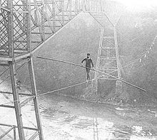
Часто мы слышим выражения: «он инертный», «двигаться по инерции», «момент инерции». В переносном значении слово «инерция» может трактоваться как отсутствие инициативы и действий. Нас же интересует прямое значение.
Ежедневная рассылка с полезной информацией для студентов всех направлений – на нашем телеграм-канале.
Что такое инерция
Согласно определению инерция в физике – это способность тел сохранять состояние покоя или движения в отсутствие действия внешних сил.
Если с самим понятием инерции все понятно на интуитивном уровне, то момент инерции – отдельный вопрос. Согласитесь, сложно представить в уме, что это такое. В этой статье Вы научитесь решать базовые задачи на тему «Момент инерции».
Определение момента инерции
Из школьного курса известно, что масса – мера инертности тела. Если мы толкнем две тележки разной массы, то остановить сложнее будет ту, которая тяжелее. То есть чем больше масса, тем большее внешнее воздействие необходимо, чтобы изменить движение тела. Рассмотренное относится к поступательному движению, когда тележка из примера движется по прямой.

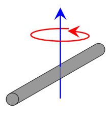
По аналогии с массой и поступательным движением момент инерции – это мера инертности тела при вращательном движении вокруг оси.
Момент инерции – скалярная физическая величина, мера инертности тела при вращении вокруг оси. Обозначается буквой J и в системе СИ измеряется в килограммах, умноженных на квадратный метр.
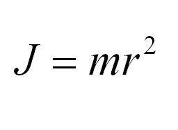
Как посчитать момент инерции? Есть общая формула, по которой в физике вычисляется момент инерции любого тела. Если тело разбить на бесконечно малые кусочки массой dm, то момент инерции будет равен сумме произведений этих элементарных масс на квадрат расстояния до оси вращения.

Это общая формула для момента инерции в физике. Для материальной точки массы m, вращающейся вокруг оси на расстоянии r от нее, данная формула принимает вид:
Теорема Штейнера
От чего зависит момент инерции? От массы, положения оси вращения, формы и размеров тела.
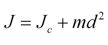
Теорема Гюйгенса-Штейнера – очень важная теорема, которую часто используют при решении задач.
Кстати! Для наших читателей сейчас действует скидка 10% на любой вид работы
Теорема Гюйгенса-Штейнера гласит:
Момент инерции тела относительно произвольной оси равняется сумме момента инерции тела относительно оси, проходящей через центр масс параллельно произвольной оси и произведения массы тела на квадрат расстояния между осями.
Для тех, кто не хочет постоянно интегрировать при решении задач на нахождение момента инерции, приведем рисунок с указанием моментов инерции некоторых однородных тел, которые часто встречаются в задачах:

Пример решения задачи на нахождение момента инерции
Рассмотрим два примера. Первая задача – на нахождение момента инерции. Вторая задача – на использование теоремы Гюйгенса-Штейнера.
Задача 1. Найти момент инерции однородного диска массы m и радиуса R. Ось вращения проходит через центр диска.
Решение:
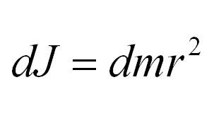
Разобьем диск на бесконечно тонкие кольца, радиус которых меняется от 0 до R и рассмотрим одно такое кольцо. Пусть его радиус – r, а масса – dm. Тогда момент инерции кольца:
Массу кольца можно представить в виде:

Здесь dz – высота кольца. Подставим массу в формулу для момента инерции и проинтегрируем:

В итоге получилась формула для момента инерции абсолютного тонкого диска или цилиндра.
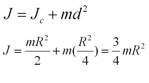
Задача 2. Пусть опять есть диск массы m и радиуса R. Теперь нужно найти момент инерции диска относительно оси, проходящей через середину одного из его радиусов.
Решение:
Момент инерции диска относительно оси, проходящей через центр масс, известен из предыдущей задачи. Применим теорему Штейнера и найдем:
Кстати, в нашем блоге Вы можете найти и другие полезные материалы по физике и решению задач.
Надеемся, что Вы найдете в статье что-то полезное для себя. Если в процессе расчета тензора инерции возникают трудности, не забывайте о студенческом сервисе. Наши специалисты проконсультируют по любому вопросу и помогут решить задачу в считанные минуты.

Иван Колобков, известный также как Джони. Маркетолог, аналитик и копирайтер компании Zaochnik. Подающий надежды молодой писатель. Питает любовь к физике, раритетным вещам и творчеству Ч. Буковски.
Момент
инерции —
скалярная
физическая величина, характеризующая
распределение масс в теле, равная сумме
произведений элементарных масс на
квадрат их расстояний до базового
множества (точки, прямой или плоскости).
Единица
измерения СИ: кг·м².
Обозначение:
I
или J.
 Для
Для
расчета моментов
инерции
тонкого диска
массы m
и радиуса R
выберем систему координат так, чтобы
ее оси совпадали с главными центральными
осями (рис.32). Определим момент инерции
тонкого однородного диска относительно
оси z
, перпендикулярной к плоскости диска.
Рассмотрим бесконечно тонкое кольцо с
внутренним
радиусом
r
и наружным r+dr.
Площадь такого кольца ds=2r
$pi$ dr, а его
масса
![]() ,
,
гдеS= $pi$ R2
— площадь всего диска. Момент инерции
тонкого кольца найдется по формуле
dJ=dmr2.
Момент инерции всего диска определяется
интегралом
![]()
Вычисление
момента
инерции тонкого стержня:
Пусть
тонкий стержень имеет длину l
и массу m.
Разделим его на малые элементы длины
dx
(рис.27), масса которых
![]() .
.
Если выбранный элемент находится на
расстоянии x от оси, то его момент инерции![]() ,
,
т.е.![]()
Интегрируя
последнее соотношение в пределах от 0
до l/2
и удваивая полученное выражение (для
учета левой половины стержня), получим
![]()
Момент
инеpции обручаотносительно оси,
пpоходящей чеpез центp кольца пеpпендикуляpно
к его плоскости. В этом случае все
элементаpные массы обруча удалены от
оси на одинаковое pасстояние, поэтому
в сумме (3.18) r2 можно вынести за знак
суммы, т. е.![]()
Теорема
Штейнера:
В
общем случае вращения тела произвольной
формы вокруг произвольной оси, вычисление
момента инерции может быть произведено
с помощью теоремы Штейнера: момент
инерции относительно произвольной оси
равен сумме момента инерции J0 относительно
оси, параллельной данной и проходящей
через центр инерции тела, и произведения
массы тела на квадрат расстояния между
осями: J=J0+ma^2.
Например,
момент инерции диска относительно оси
О’ в соответствии с теоремой Штейнера:
![]()
17. Момент инерции однородного тела вращения. Моменты инерции конуса, шара.
Линия
![]() — ось вращения.
— ось вращения.
![]() — масса на квадрат радиуса окружности,
— масса на квадрат радиуса окружности,
по которой движется материальная точка.
Все
тело мысленно разбиваем на маленькие
объемы. Масса этого кусочка
![]() .
.
![]()
Твердое
тело представляется как совокупность
системы точечных масс.
![]() — расстояние, на котором находится точка
— расстояние, на котором находится точка
от оси вращения.
![]()
![]() — общий алгоритм определения собственного
— общий алгоритм определения собственного
момента инерции твердого тела, относительно
оси проходящей через центр инерции
данного тела.
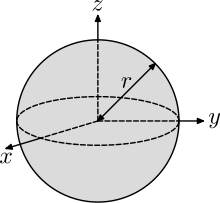
Момент
инерции шара.
Сплошной шар массы
m
и радиуса R
можно рассматривать как совокупность
бесконечно тонких сферических слоев с
массами dm
, радиусом r,
толщиной dr
(рис.35).

Рассмотрим
малый элемент сферического слоя $delta$
m с координатами
x, y, z.
Его моменты инерции относительно осей
проходящих через центр слоя — $delta$
Jx,
$delta$ Jy,
$delta$ Jz,
равны
![]()
Т.
е. можно записать
![]() (п.26)
(п.26)
Так как для
элементов сферического слоя x2+y2+z2=r2
то
![]()
После
интегрирования по всему объему слоя
получим
![]() (п.27)
(п.27)
Так как, в силу
симметрии для сферического слоя
dJx=dJy=dJz=dJ
, а
 ,
,
то![]() Интегрируя по всему объему шара,
Интегрируя по всему объему шара,
получаем![]()
Окончательно
(после интегрирования) получим, что
момент инерции шара относительно оси,
проходящей через его центр равен
![]()
Разобьём
КОНУС
на цилиндрические слои
ось
толщиной dr.
Масса такого слоя
dm
= r2dr,
где
ρ – плотность
материала, из которого изготовлен конус.
Момент инерции этого слоя
dI = dm.r2.
Момент
инерции всего конуса
складывается
из моментов инерции всех слоёв:
I
=
![]() =
=
![]() ρπ
ρπ
r
4
dr
=
![]() ρR5.
ρR5.
Остаётся выразить
его через массу всего цилиндра:
m
=
![]() =
=
![]() =
=
![]() R3,
R3,
отсюда ρ
=
![]() ,
,
I
=
![]() =
=
![]() mR2.
mR2.
Соседние файлы в предмете [НЕСОРТИРОВАННОЕ]
- #
- #
- #
- #
- #
- #
- #
- #
- #
- #
- #
For the quantity also known as the «area moment of inertia», see Second moment of area.
| Moment of inertia | |
|---|---|

Flywheels have large moments of inertia to smooth out changes in rates of rotational motion. |
|
|
Common symbols |
I |
| SI unit | kg⋅m2 |
|
Other units |
lbf·ft·s2 |
|
Derivations from |
 |
| Dimension | M L2 |


To improve their maneuverability, war planes are designed to have smaller moments of inertia compared to commercial planes.
The moment of inertia, otherwise known as the mass moment of inertia, angular mass, second moment of mass, or most accurately, rotational inertia, of a rigid body is a quantity that determines the torque needed for a desired angular acceleration about a rotational axis, akin to how mass determines the force needed for a desired acceleration. It depends on the body’s mass distribution and the axis chosen, with larger moments requiring more torque to change the body’s rate of rotation.
It is an extensive (additive) property: for a point mass the moment of inertia is simply the mass times the square of the perpendicular distance to the axis of rotation. The moment of inertia of a rigid composite system is the sum of the moments of inertia of its component subsystems (all taken about the same axis). Its simplest definition is the second moment of mass with respect to distance from an axis.
For bodies constrained to rotate in a plane, only their moment of inertia about an axis perpendicular to the plane, a scalar value, matters. For bodies free to rotate in three dimensions, their moments can be described by a symmetric 3-by-3 matrix, with a set of mutually perpendicular principal axes for which this matrix is diagonal and torques around the axes act independently of each other.
Introduction[edit]
When a body is free to rotate around an axis, torque must be applied to change its angular momentum. The amount of torque needed to cause any given angular acceleration (the rate of change in angular velocity) is proportional to the moment of inertia of the body. Moments of inertia may be expressed in units of kilogram metre squared (kg·m2) in SI units and pound-foot-second squared (lbf·ft·s2) in imperial or US units.
The moment of inertia plays the role in rotational kinetics that mass (inertia) plays in linear kinetics—both characterize the resistance of a body to changes in its motion. The moment of inertia depends on how mass is distributed around an axis of rotation, and will vary depending on the chosen axis. For a point-like mass, the moment of inertia about some axis is given by  , where
  is the distance of the point from the axis, and
  is the mass. For an extended rigid body, the moment of inertia is just the sum of all the small pieces of mass multiplied by the square of their distances from the axis in rotation. For an extended body of a regular shape and uniform density, this summation sometimes produces a simple expression that depends on the dimensions, shape and total mass of the object.
In 1673 Christiaan Huygens introduced this parameter in his study of the oscillation of a body hanging from a pivot, known as a compound pendulum.[1] The term moment of inertia («momentum inertiae» in Latin) was introduced by Leonhard Euler in his book Theoria motus corporum solidorum seu rigidorum in 1765,[1][2] and it is incorporated into Euler’s second law.
The natural frequency of oscillation of a compound pendulum is obtained from the ratio of the torque imposed by gravity on the mass of the pendulum to the resistance to acceleration defined by the moment of inertia. Comparison of this natural frequency to that of a simple pendulum consisting of a single point of mass provides a mathematical formulation for moment of inertia of an extended body.[3][4]
The moment of inertia also appears in momentum, kinetic energy, and in Newton’s laws of motion for a rigid body as a physical parameter that combines its shape and mass. There is an interesting difference in the way moment of inertia appears in planar and spatial movement. Planar movement has a single scalar that defines the moment of inertia, while for spatial movement the same calculations yield a 3 × 3 matrix of moments of inertia, called the inertia matrix or inertia tensor.[5][6]
The moment of inertia of a rotating flywheel is used in a machine to resist variations in applied torque to smooth its rotational output. The moment of inertia of an airplane about its longitudinal, horizontal and vertical axes determine how steering forces on the control surfaces of its wings, elevators and rudder(s) affect the plane’s motions in roll, pitch and yaw.
Definition[edit]
The moment of inertia is defined as the product of mass of section and the square of the distance between the reference axis and the centroid of the section.

Video of rotating chair experiment, illustrating moment of inertia. When the spinning professor pulls his arms, his moment of inertia decreases; to conserve angular momentum, his angular velocity increases.
The moment of inertia I is also defined as the ratio of the net angular momentum L of a system to its angular velocity ω around a principal axis,[7][8] that is

If the angular momentum of a system is constant, then as the moment of inertia gets smaller, the angular velocity must increase. This occurs when spinning figure skaters pull in their outstretched arms or divers curl their bodies into a tuck position during a dive, to spin faster.[7][8][9][10][11][12][13]
If the shape of the body does not change, then its moment of inertia appears in Newton’s law of motion as the ratio of an applied torque τ on a body to the angular acceleration α around a principal axis, that is

For a simple pendulum, this definition yields a formula for the moment of inertia I in terms of the mass m of the pendulum and its distance r from the pivot point as,

Thus, the moment of inertia of the pendulum depends on both the mass m of a body and its geometry, or shape, as defined by the distance r to the axis of rotation.
This simple formula generalizes to define moment of inertia for an arbitrarily shaped body as the sum of all the elemental point masses dm each multiplied by the square of its perpendicular distance r to an axis k. An arbitrary object’s moment of inertia thus depends on the spatial distribution of its mass.
In general, given an object of mass m, an effective radius k can be defined, dependent on a particular axis of rotation, with such a value that its moment of inertia around the axis is

where k is known as the radius of gyration around the axis.
Examples[edit]
Simple pendulum[edit]
Mathematically, the moment of inertia of a simple pendulum is the ratio of the torque due to gravity about the pivot of a pendulum to its angular acceleration about that pivot point. For a simple pendulum this is found to be the product of the mass of the particle with the square of its distance to the pivot, that is
This can be shown as follows: The force of gravity on the mass of a simple pendulum generates a torque  around the axis perpendicular to the plane of the pendulum movement. Here
  is the distance vector from the torque axis to the pendulum center of mass, and
  is the net force on the mass. Associated with this torque is an angular acceleration,
  , of the string and mass around this axis. Since the mass is constrained to a circle the tangential acceleration of the mass is
  . Since
  the torque equation becomes:

where  is a unit vector perpendicular to the plane of the pendulum. (The second to last step uses the vector triple product expansion with the perpendicularity of and .) The quantity
  is the moment of inertia of this single mass around the pivot point.
The quantity also appears in the angular momentum of a simple pendulum, which is calculated from the velocity  of the pendulum mass around the pivot, where
  is the angular velocity of the mass about the pivot point. This angular momentum is given by

using a similar derivation to the previous equation.
Similarly, the kinetic energy of the pendulum mass is defined by the velocity of the pendulum around the pivot to yield

This shows that the quantity is how mass combines with the shape of a body to define rotational inertia. The moment of inertia of an arbitrarily shaped body is the sum of the values for all of the elements of mass in the body.
Compound pendulums[edit]

Pendulums used in Mendenhall gravimeter apparatus, from 1897 scientific journal. The portable gravimeter developed in 1890 by Thomas C. Mendenhall provided the most accurate relative measurements of the local gravitational field of the Earth.
A compound pendulum is a body formed from an assembly of particles of continuous shape that rotates rigidly around a pivot. Its moment of inertia is the sum of the moments of inertia of each of the particles that it is composed of.[14][15]: 395–396 [16]: 51–53 The natural frequency ( ) of a compound pendulum depends on its moment of inertia,
  ,
,

where is the mass of the object,  is local acceleration of gravity, and is the distance from the pivot point to the center of mass of the object. Measuring this frequency of oscillation over small angular displacements provides an effective way of measuring moment of inertia of a body.[17]: 516–517
Thus, to determine the moment of inertia of the body, simply suspend it from a convenient pivot point  so that it swings freely in a plane perpendicular to the direction of the desired moment of inertia, then measure its natural frequency or period of oscillation (
 ), to obtain

where is the period (duration) of oscillation (usually averaged over multiple periods).
Center of oscillation[edit]
A simple pendulum that has the same natural frequency as a compound pendulum defines the length  from the pivot to a point called the center of oscillation of the compound pendulum. This point also corresponds to the center of percussion. The length is determined from the formula,

or

The seconds pendulum, which provides the «tick» and «tock» of a grandfather clock, takes one second to swing from side-to-side. This is a period of two seconds, or a natural frequency of  for the pendulum. In this case, the distance to the center of oscillation, , can be computed to be

Notice that the distance to the center of oscillation of the seconds pendulum must be adjusted to accommodate different values for the local acceleration of gravity. Kater’s pendulum is a compound pendulum that uses this property to measure the local acceleration of gravity, and is called a gravimeter.
Measuring moment of inertia[edit]
The moment of inertia of a complex system such as a vehicle or airplane around its vertical axis can be measured by suspending the system from three points to form a trifilar pendulum. A trifilar pendulum is a platform supported by three wires designed to oscillate in torsion around its vertical centroidal axis.[18] The period of oscillation of the trifilar pendulum yields the moment of inertia of the system.[19]
Moment of inertia of area[edit]
Moment of inertia of area is also known as the second moment of area.
These calculations are commonly used in civil engineering for structural design of beams and columns. Cross-sectional areas calculated for vertical moment of the x-axis  and horizontal moment of the y-axis
  .
.
Height (h) and breadth (b) are the linear measures, except for circles, which are effectively half-breadth derived,
Sectional areas moment calculated thus[20][edit]
- Square:

- Rectangular: and;
- Triangular:
- Circular:


Motion in a fixed plane[edit]
Point mass[edit]
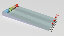
Four objects with identical masses and radii racing down a plane while rolling without slipping.
From back to front:
- spherical shell,
- solid sphere,
- cylindrical ring, and
- solid cylinder.
The time for each object to reach the finishing line depends on their moment of inertia. (OGV version)
The moment of inertia about an axis of a body is calculated by summing for every particle in the body, where is the perpendicular distance to the specified axis. To see how moment of inertia arises in the study of the movement of an extended body, it is convenient to consider a rigid assembly of point masses. (This equation can be used for axes that are not principal axes provided that it is understood that this does not fully describe the moment of inertia.[21])
Consider the kinetic energy of an assembly of  masses
  that lie at the distances
  from the pivot point , which is the nearest point on the axis of rotation. It is the sum of the kinetic energy of the individual masses,[17]: 516–517 [22]: 1084–1085 [22]: 1296–1300

This shows that the moment of inertia of the body is the sum of each of the terms, that is

Thus, moment of inertia is a physical property that combines the mass and distribution of the particles around the rotation axis. Notice that rotation about different axes of the same body yield different moments of inertia.
The moment of inertia of a continuous body rotating about a specified axis is calculated in the same way, except with infinitely many point particles. Thus the limits of summation are removed, and the sum is written as follows:

Another expression replaces the summation with an integral,

Here, the function  gives the mass density at each point
  , is a vector perpendicular to the axis of rotation and extending from a point on the rotation axis to a point in the solid, and the integration is evaluated over the volume
  of the body
  . The moment of inertia of a flat surface is similar with the mass density being replaced by its areal mass density with the integral evaluated over its area.
Note on second moment of area: The moment of inertia of a body moving in a plane and the second moment of area of a beam’s cross-section are often confused. The moment of inertia of a body with the shape of the cross-section is the second moment of this area about the  -axis perpendicular to the cross-section, weighted by its density. This is also called the polar moment of the area, and is the sum of the second moments about the
  — and
— and  -axes.[23] The stresses in a beam are calculated using the second moment of the cross-sectional area around either the -axis or -axis depending on the load.
Examples[edit]
The moment of inertia of a compound pendulum constructed from a thin disc mounted at the end of a thin rod that oscillates around a pivot at the other end of the rod, begins with the calculation of the moment of inertia of the thin rod and thin disc about their respective centers of mass.[22]
A list of moments of inertia formulas for standard body shapes provides a way to obtain the moment of inertia of a complex body as an assembly of simpler shaped bodies. The parallel axis theorem is used to shift the reference point of the individual bodies to the reference point of the assembly.
As one more example, consider the moment of inertia of a solid sphere of constant density about an axis through its center of mass. This is determined by summing the moments of inertia of the thin discs that can form the sphere whose centers are along the axis chosen for consideration. If the surface of the ball is defined by the equation[22]: 1301

then the square of the radius of the disc at the cross-section along the -axis is

Therefore, the moment of inertia of the ball is the sum of the moments of inertia of the discs along the -axis,
![{displaystyle {begin{aligned}I_{C,{text{ball}}}&=int _{-R}^{R}{frac {pi rho }{2}}r(z)^{4},dz=int _{-R}^{R}{frac {pi rho }{2}}left(R^{2}-z^{2}right)^{2},dz\&={frac {pi rho }{2}}left[R^{4}z-{frac {2}{3}}R^{2}z^{3}+{frac {1}{5}}z^{5}right]_{-R}^{R}\&=pi rho left(1-{frac {2}{3}}+{frac {1}{5}}right)R^{5}\&={frac {2}{5}}mR^{2},end{aligned}}}](https://wikimedia.org/api/rest_v1/media/math/render/svg/42e610139e74980c31f979cff68d8cdd3684dd05)
where  is the mass of the sphere.
Rigid body[edit]

The cylinders with higher moment of inertia roll down a slope with a smaller acceleration, as more of their potential energy needs to be converted into the rotational kinetic energy.
If a mechanical system is constrained to move parallel to a fixed plane, then the rotation of a body in the system occurs around an axis parallel to this plane. In this case, the moment of inertia of the mass in this system is a scalar known as the polar moment of inertia. The definition of the polar moment of inertia can be obtained by considering momentum, kinetic energy and Newton’s laws for the planar movement of a rigid system of particles.[14][17][24][25]
If a system of  particles,
  , are assembled into a rigid body, then the momentum of the system can be written in terms of positions relative to a reference point
  , and absolute velocities
  :
:

where is the angular velocity of the system and  is the velocity of .
For planar movement the angular velocity vector is directed along the unit vector  which is perpendicular to the plane of movement. Introduce the unit vectors
  from the reference point to a point
  , and the unit vector
  , so
, so

This defines the relative position vector and the velocity vector for the rigid system of the particles moving in a plane.
Note on the cross product: When a body moves parallel to a ground plane, the trajectories of all the points in the body lie in planes parallel to this ground plane. This means that any rotation that the body undergoes must be around an axis perpendicular to this plane. Planar movement is often presented as projected onto this ground plane so that the axis of rotation appears as a point. In this case, the angular velocity and angular acceleration of the body are scalars and the fact that they are vectors along the rotation axis is ignored. This is usually preferred for introductions to the topic. But in the case of moment of inertia, the combination of mass and geometry benefits from the geometric properties of the cross product. For this reason, in this section on planar movement the angular velocity and accelerations of the body are vectors perpendicular to the ground plane, and the cross product operations are the same as used for the study of spatial rigid body movement.
Angular momentum[edit]
The angular momentum vector for the planar movement of a rigid system of particles is given by[14][17]

Use the center of mass  as the reference point so

and define the moment of inertia relative to the center of mass  as
as

then the equation for angular momentum simplifies to[22]: 1028

The moment of inertia about an axis perpendicular to the movement of the rigid system and through the center of mass is known as the polar moment of inertia. Specifically, it is the second moment of mass with respect to the orthogonal distance from an axis (or pole).
For a given amount of angular momentum, a decrease in the moment of inertia results in an increase in the angular velocity. Figure skaters can change their moment of inertia by pulling in their arms. Thus, the angular velocity achieved by a skater with outstretched arms results in a greater angular velocity when the arms are pulled in, because of the reduced moment of inertia. A figure skater is not, however, a rigid body.
Kinetic energy[edit]

This 1906 rotary shear uses the moment of inertia of two flywheels to store kinetic energy which when released is used to cut metal stock (International Library of Technology, 1906).
The kinetic energy of a rigid system of particles moving in the plane is given by[14][17]

Let the reference point be the center of mass of the system so the second term becomes zero, and introduce the moment of inertia so the kinetic energy is given by[22]: 1084

The moment of inertia is the polar moment of inertia of the body.
Newton’s laws[edit]

A 1920s John Deere tractor with the spoked flywheel on the engine. The large moment of inertia of the flywheel smooths the operation of the tractor.
Newton’s laws for a rigid system of particles, , can be written in terms of a resultant force and torque at a reference point , to yield[14][17]

where denotes the trajectory of each particle.
The kinematics of a rigid body yields the formula for the acceleration of the particle  in terms of the position and acceleration
  of the reference particle as well as the angular velocity vector and angular acceleration vector of the rigid system of particles as,

For systems that are constrained to planar movement, the angular velocity and angular acceleration vectors are directed along perpendicular to the plane of movement, which simplifies this acceleration equation. In this case, the acceleration vectors can be simplified by introducing the unit vectors  from the reference point to a point and the unit vectors , so

This yields the resultant torque on the system as

where  , and
, and  is the unit vector perpendicular to the plane for all of the particles .
Use the center of mass as the reference point and define the moment of inertia relative to the center of mass , then the equation for the resultant torque simplifies to[22]: 1029

Motion in space of a rigid body, and the inertia matrix[edit]
The scalar moments of inertia appear as elements in a matrix when a system of particles is assembled into a rigid body that moves in three-dimensional space. This inertia matrix appears in the calculation of the angular momentum, kinetic energy and resultant torque of the rigid system of particles.[3][4][5][6][26]
Let the system of particles, be located at the coordinates with velocities relative to a fixed reference frame. For a (possibly moving) reference point , the relative positions are

and the (absolute) velocities are

where is the angular velocity of the system, and  is the velocity of .
Angular momentum[edit]
Note that the cross product can be equivalently written as matrix multiplication by combining the first operand and the operator into a skew-symmetric matrix, ![{displaystyle left[mathbf {b} right]}](https://wikimedia.org/api/rest_v1/media/math/render/svg/2ce9643510bd433e0ed612edd5d3a9ed7faecfec) , constructed from the components of
, constructed from the components of  :
:
![{displaystyle {begin{aligned}mathbf {b} times mathbf {y} &equiv left[mathbf {b} right]mathbf {y} \left[mathbf {b} right]&equiv {begin{bmatrix}0&-b_{z}&b_{y}\b_{z}&0&-b_{x}\-b_{y}&b_{x}&0end{bmatrix}}.end{aligned}}}](https://wikimedia.org/api/rest_v1/media/math/render/svg/b4782eb664e98a6d680dd96b77601ff9bc12ab4a)
The inertia matrix is constructed by considering the angular momentum, with the reference point of the body chosen to be the center of mass :[3][6]

where the terms containing ( ) sum to zero by the definition of center of mass.
Then, the skew-symmetric matrix ![{displaystyle [Delta mathbf {r} _{i}]}](https://wikimedia.org/api/rest_v1/media/math/render/svg/3ee5960e77611f673ab2f2050f356dbf0e403132) obtained from the relative position vector
obtained from the relative position vector  , can be used to define,
![{displaystyle mathbf {L} =left(-sum _{i=1}^{n}m_{i}left[Delta mathbf {r} _{i}right]^{2}right){boldsymbol {omega }}=mathbf {I} _{mathbf {C} }{boldsymbol {omega }},}](https://wikimedia.org/api/rest_v1/media/math/render/svg/26ff4f4ab9aa3fff11085b8828fc71a4af7de700)
where  defined by
![{displaystyle mathbf {I} _{mathbf {C} }=-sum _{i=1}^{n}m_{i}left[Delta mathbf {r} _{i}right]^{2},}](https://wikimedia.org/api/rest_v1/media/math/render/svg/6766e8a9ce07ff8f32ec86aaa929f1e5a3ce1a21)
is the symmetric inertia matrix of the rigid system of particles measured relative to the center of mass .
Kinetic energy[edit]
The kinetic energy of a rigid system of particles can be formulated in terms of the center of mass and a matrix of mass moments of inertia of the system. Let the system of particles be located at the coordinates with velocities , then the kinetic energy is[3][6]

where is the position vector of a particle relative to the center of mass.
This equation expands to yield three terms

Since the center of mass is defined by

, the second term in this equation is zero. Introduce the skew-symmetric matrix so the kinetic energy becomes
![{displaystyle {begin{aligned}E_{text{K}}&={frac {1}{2}}left(sum _{i=1}^{n}m_{i}left(left[Delta mathbf {r} _{i}right]{boldsymbol {omega }}right)cdot left(left[Delta mathbf {r} _{i}right]{boldsymbol {omega }}right)right)+{frac {1}{2}}left(sum _{i=1}^{n}m_{i}right)mathbf {V} _{mathbf {C} }cdot mathbf {V} _{mathbf {C} }\&={frac {1}{2}}left(sum _{i=1}^{n}m_{i}left({boldsymbol {omega }}^{mathsf {T}}left[Delta mathbf {r} _{i}right]^{mathsf {T}}left[Delta mathbf {r} _{i}right]{boldsymbol {omega }}right)right)+{frac {1}{2}}left(sum _{i=1}^{n}m_{i}right)mathbf {V} _{mathbf {C} }cdot mathbf {V} _{mathbf {C} }\&={frac {1}{2}}{boldsymbol {omega }}cdot left(-sum _{i=1}^{n}m_{i}left[Delta mathbf {r} _{i}right]^{2}right){boldsymbol {omega }}+{frac {1}{2}}left(sum _{i=1}^{n}m_{i}right)mathbf {V} _{mathbf {C} }cdot mathbf {V} _{mathbf {C} }.end{aligned}}}](https://wikimedia.org/api/rest_v1/media/math/render/svg/2c246c5646e149b67a600084c164f154ec7dda89)
Thus, the kinetic energy of the rigid system of particles is given by

where is the inertia matrix relative to the center of mass and  is the total mass.
Resultant torque[edit]
The inertia matrix appears in the application of Newton’s second law to a rigid assembly of particles. The resultant torque on this system is,[3][6]

where  is the acceleration of the particle . The kinematics of a rigid body yields the formula for the acceleration of the particle in terms of the position and acceleration
  of the reference point, as well as the angular velocity vector and angular acceleration vector of the rigid system as,

Use the center of mass as the reference point, and introduce the skew-symmetric matrix ![{displaystyle left[Delta mathbf {r} _{i}right]=left[mathbf {r} _{i}-mathbf {C} right]}](https://wikimedia.org/api/rest_v1/media/math/render/svg/9b83ab9af0efe0f59204a493b10b5eb453594c19) to represent the cross product
to represent the cross product  , to obtain
![{displaystyle {boldsymbol {tau }}=left(-sum _{i=1}^{n}m_{i}left[Delta mathbf {r} _{i}right]^{2}right){boldsymbol {alpha }}+{boldsymbol {omega }}times left(-sum _{i=1}^{n}m_{i}left[Delta mathbf {r} _{i}right]^{2}right){boldsymbol {omega }}}](https://wikimedia.org/api/rest_v1/media/math/render/svg/b93d7ec560fb15fbaaba36a2fd0869da807fd92e)
The calculation uses the identity

obtained from the Jacobi identity for the triple cross product as shown in the proof below:
Proof
![{displaystyle {begin{aligned}{boldsymbol {tau }}&=sum _{i=1}^{n}(mathbf {r_{i}} -mathbf {R} )times (m_{i}mathbf {a} _{i})\&=sum _{i=1}^{n}{boldsymbol {Delta }}mathbf {r} _{i}times (m_{i}mathbf {a} _{i})\&=sum _{i=1}^{n}m_{i}[{boldsymbol {Delta }}mathbf {r} _{i}times mathbf {a} _{i}];ldots {text{ cross-product scalar multiplication}}\&=sum _{i=1}^{n}m_{i}[{boldsymbol {Delta }}mathbf {r} _{i}times (mathbf {a} _{{text{tangential}},i}+mathbf {a} _{{text{centripetal}},i}+mathbf {A} _{mathbf {R} })]\&=sum _{i=1}^{n}m_{i}[{boldsymbol {Delta }}mathbf {r} _{i}times (mathbf {a} _{{text{tangential}},i}+mathbf {a} _{{text{centripetal}},i}+0)]\&;;;;;ldots ;mathbf {R} {text{ is either at rest or moving at a constant velocity but not accelerated, or }}\&;;;;;;;;;;;{text{the origin of the fixed (world) coordinate reference system is placed at the center of mass }}mathbf {C} \&=sum _{i=1}^{n}m_{i}[{boldsymbol {Delta }}mathbf {r} _{i}times mathbf {a} _{{text{tangential}},i}+{boldsymbol {Delta }}mathbf {r} _{i}times mathbf {a} _{{text{centripetal}},i}];ldots {text{ cross-product distributivity over addition}}\&=sum _{i=1}^{n}m_{i}[{boldsymbol {Delta }}mathbf {r} _{i}times ({boldsymbol {alpha }}times {boldsymbol {Delta }}mathbf {r} _{i})+{boldsymbol {Delta }}mathbf {r} _{i}times ({boldsymbol {omega }}times mathbf {v} _{{text{tangential}},i})]\{boldsymbol {tau }}&=sum _{i=1}^{n}m_{i}[{boldsymbol {Delta }}mathbf {r} _{i}times ({boldsymbol {alpha }}times {boldsymbol {Delta }}mathbf {r} _{i})+{boldsymbol {Delta }}mathbf {r} _{i}times ({boldsymbol {omega }}times ({boldsymbol {omega }}times {boldsymbol {Delta }}mathbf {r} _{i}))]\end{aligned}}}](https://wikimedia.org/api/rest_v1/media/math/render/svg/3a1a1b0804a6cf8a550a81732385fca1083051df)
Then, the following Jacobi identity is used on the last term:
![{displaystyle {begin{aligned}0&={boldsymbol {Delta }}mathbf {r} _{i}times ({boldsymbol {omega }}times ({boldsymbol {omega }}times {boldsymbol {Delta }}mathbf {r} _{i}))+{boldsymbol {omega }}times (({boldsymbol {omega }}times {boldsymbol {Delta }}mathbf {r} _{i})times {boldsymbol {Delta }}mathbf {r} _{i})+({boldsymbol {omega }}times {boldsymbol {Delta }}mathbf {r} _{i})times ({boldsymbol {Delta }}mathbf {r} _{i}times {boldsymbol {omega }})\&={boldsymbol {Delta }}mathbf {r} _{i}times ({boldsymbol {omega }}times ({boldsymbol {omega }}times {boldsymbol {Delta }}mathbf {r} _{i}))+{boldsymbol {omega }}times (({boldsymbol {omega }}times {boldsymbol {Delta }}mathbf {r} _{i})times {boldsymbol {Delta }}mathbf {r} _{i})+({boldsymbol {omega }}times {boldsymbol {Delta }}mathbf {r} _{i})times -({boldsymbol {omega }}times {boldsymbol {Delta }}mathbf {r} _{i});ldots {text{ cross-product anticommutativity}}\&={boldsymbol {Delta }}mathbf {r} _{i}times ({boldsymbol {omega }}times ({boldsymbol {omega }}times {boldsymbol {Delta }}mathbf {r} _{i}))+{boldsymbol {omega }}times (({boldsymbol {omega }}times {boldsymbol {Delta }}mathbf {r} _{i})times {boldsymbol {Delta }}mathbf {r} _{i})+-[({boldsymbol {omega }}times {boldsymbol {Delta }}mathbf {r} _{i})times ({boldsymbol {omega }}times {boldsymbol {Delta }}mathbf {r} _{i})];ldots {text{ cross-product scalar multiplication}}\&={boldsymbol {Delta }}mathbf {r} _{i}times ({boldsymbol {omega }}times ({boldsymbol {omega }}times {boldsymbol {Delta }}mathbf {r} _{i}))+{boldsymbol {omega }}times (({boldsymbol {omega }}times {boldsymbol {Delta }}mathbf {r} _{i})times {boldsymbol {Delta }}mathbf {r} _{i})+-[0];ldots {text{ self cross-product}}\0&={boldsymbol {Delta }}mathbf {r} _{i}times ({boldsymbol {omega }}times ({boldsymbol {omega }}times {boldsymbol {Delta }}mathbf {r} _{i}))+{boldsymbol {omega }}times (({boldsymbol {omega }}times {boldsymbol {Delta }}mathbf {r} _{i})times {boldsymbol {Delta }}mathbf {r} _{i})end{aligned}}}](https://wikimedia.org/api/rest_v1/media/math/render/svg/88ab33d54b34674092a14d55c8ccefb765a2e7ae)
The result of applying Jacobi identity can then be continued as follows:
![{displaystyle {begin{aligned}{boldsymbol {Delta }}mathbf {r} _{i}times ({boldsymbol {omega }}times ({boldsymbol {omega }}times {boldsymbol {Delta }}mathbf {r} _{i}))&=-[{boldsymbol {omega }}times (({boldsymbol {omega }}times {boldsymbol {Delta }}mathbf {r} _{i})times {boldsymbol {Delta }}mathbf {r} _{i})]\&=-[({boldsymbol {omega }}times {boldsymbol {Delta }}mathbf {r} _{i})({boldsymbol {omega }}cdot {boldsymbol {Delta }}mathbf {r} _{i})-{boldsymbol {Delta }}mathbf {r} _{i}({boldsymbol {omega }}cdot ({boldsymbol {omega }}times {boldsymbol {Delta }}mathbf {r} _{i}))];ldots {text{ vector triple product}}\&=-[({boldsymbol {omega }}times {boldsymbol {Delta }}mathbf {r} _{i})({boldsymbol {omega }}cdot {boldsymbol {Delta }}mathbf {r} _{i})-{boldsymbol {Delta }}mathbf {r} _{i}({boldsymbol {Delta }}mathbf {r} _{i}cdot ({boldsymbol {omega }}times {boldsymbol {omega }}))];ldots {text{ scalar triple product}}\&=-[({boldsymbol {omega }}times {boldsymbol {Delta }}mathbf {r} _{i})({boldsymbol {omega }}cdot {boldsymbol {Delta }}mathbf {r} _{i})-{boldsymbol {Delta }}mathbf {r} _{i}({boldsymbol {Delta }}mathbf {r} _{i}cdot (0))];ldots {text{ self cross-product}}\&=-[({boldsymbol {omega }}times {boldsymbol {Delta }}mathbf {r} _{i})({boldsymbol {omega }}cdot {boldsymbol {Delta }}mathbf {r} _{i})]\&=-[{boldsymbol {omega }}times ({boldsymbol {Delta }}mathbf {r} _{i}({boldsymbol {omega }}cdot {boldsymbol {Delta }}mathbf {r} _{i}))];ldots {text{ cross-product scalar multiplication}}\&={boldsymbol {omega }}times -({boldsymbol {Delta }}mathbf {r} _{i}({boldsymbol {omega }}cdot {boldsymbol {Delta }}mathbf {r} _{i}));ldots {text{ cross-product scalar multiplication}}\{boldsymbol {Delta }}mathbf {r} _{i}times ({boldsymbol {omega }}times ({boldsymbol {omega }}times {boldsymbol {Delta }}mathbf {r} _{i}))&={boldsymbol {omega }}times -({boldsymbol {Delta }}mathbf {r} _{i}({boldsymbol {Delta }}mathbf {r} _{i}cdot {boldsymbol {omega }}));ldots {text{ dot-product commutativity}}\end{aligned}}}](https://wikimedia.org/api/rest_v1/media/math/render/svg/bb1ab7d45bf04c0df3101e84282bc6695ddecf68)
The final result can then be substituted to the main proof as follows:
![{displaystyle {begin{aligned}{boldsymbol {tau }}&=sum _{i=1}^{n}m_{i}[{boldsymbol {Delta }}mathbf {r} _{i}times ({boldsymbol {alpha }}times {boldsymbol {Delta }}mathbf {r} _{i})+{boldsymbol {Delta }}mathbf {r} _{i}times ({boldsymbol {omega }}times ({boldsymbol {omega }}times {boldsymbol {Delta }}mathbf {r} _{i}))]\&=sum _{i=1}^{n}m_{i}[{boldsymbol {Delta }}mathbf {r} _{i}times ({boldsymbol {alpha }}times {boldsymbol {Delta }}mathbf {r} _{i})+{boldsymbol {omega }}times -({boldsymbol {Delta }}mathbf {r} _{i}({boldsymbol {Delta }}mathbf {r} _{i}cdot {boldsymbol {omega }}))]\&=sum _{i=1}^{n}m_{i}[{boldsymbol {Delta }}mathbf {r} _{i}times ({boldsymbol {alpha }}times {boldsymbol {Delta }}mathbf {r} _{i})+{boldsymbol {omega }}times {0-{boldsymbol {Delta }}mathbf {r} _{i}({boldsymbol {Delta }}mathbf {r} _{i}cdot {boldsymbol {omega }})}]\&=sum _{i=1}^{n}m_{i}[{boldsymbol {Delta }}mathbf {r} _{i}times ({boldsymbol {alpha }}times {boldsymbol {Delta }}mathbf {r} _{i})+{boldsymbol {omega }}times {[{boldsymbol {omega }}({boldsymbol {Delta }}mathbf {r} _{i}cdot {boldsymbol {Delta }}mathbf {r} _{i})-{boldsymbol {omega }}({boldsymbol {Delta }}mathbf {r} _{i}cdot {boldsymbol {Delta }}mathbf {r} _{i})]-{boldsymbol {Delta }}mathbf {r} _{i}({boldsymbol {Delta }}mathbf {r} _{i}cdot {boldsymbol {omega }})}];ldots ;{boldsymbol {omega }}({boldsymbol {Delta }}mathbf {r} _{i}cdot {boldsymbol {Delta }}mathbf {r} _{i})-{boldsymbol {omega }}({boldsymbol {Delta }}mathbf {r} _{i}cdot {boldsymbol {Delta }}mathbf {r} _{i})=0\&=sum _{i=1}^{n}m_{i}[{boldsymbol {Delta }}mathbf {r} _{i}times ({boldsymbol {alpha }}times {boldsymbol {Delta }}mathbf {r} _{i})+{boldsymbol {omega }}times {[{boldsymbol {omega }}({boldsymbol {Delta }}mathbf {r} _{i}cdot {boldsymbol {Delta }}mathbf {r} _{i})-{boldsymbol {Delta }}mathbf {r} _{i}({boldsymbol {Delta }}mathbf {r} _{i}cdot {boldsymbol {omega }})]-{boldsymbol {omega }}({boldsymbol {Delta }}mathbf {r} _{i}cdot {boldsymbol {Delta }}mathbf {r} _{i})}];ldots {text{ addition associativity}}\end{aligned}}}](https://wikimedia.org/api/rest_v1/media/math/render/svg/66f6f583aacfd008f43218fc24e97547511a6a91)
![{displaystyle {begin{aligned}&=sum _{i=1}^{n}m_{i}[{boldsymbol {Delta }}mathbf {r} _{i}times ({boldsymbol {alpha }}times {boldsymbol {Delta }}mathbf {r} _{i})+{boldsymbol {omega }}times {{boldsymbol {omega }}({boldsymbol {Delta }}mathbf {r} _{i}cdot {boldsymbol {Delta }}mathbf {r} _{i})-{boldsymbol {Delta }}mathbf {r} _{i}({boldsymbol {Delta }}mathbf {r} _{i}cdot {boldsymbol {omega }})}-{boldsymbol {omega }}times {boldsymbol {omega }}({boldsymbol {Delta }}mathbf {r} _{i}cdot {boldsymbol {Delta }}mathbf {r} _{i})];ldots {text{ cross-product distributivity over addition}}\&=sum _{i=1}^{n}m_{i}[{boldsymbol {Delta }}mathbf {r} _{i}times ({boldsymbol {alpha }}times {boldsymbol {Delta }}mathbf {r} _{i})+{boldsymbol {omega }}times {{boldsymbol {omega }}({boldsymbol {Delta }}mathbf {r} _{i}cdot {boldsymbol {Delta }}mathbf {r} _{i})-{boldsymbol {Delta }}mathbf {r} _{i}({boldsymbol {Delta }}mathbf {r} _{i}cdot {boldsymbol {omega }})}-({boldsymbol {Delta }}mathbf {r} _{i}cdot {boldsymbol {Delta }}mathbf {r} _{i})({boldsymbol {omega }}times {boldsymbol {omega }})];ldots {text{ cross-product scalar multiplication}}\&=sum _{i=1}^{n}m_{i}[{boldsymbol {Delta }}mathbf {r} _{i}times ({boldsymbol {alpha }}times {boldsymbol {Delta }}mathbf {r} _{i})+{boldsymbol {omega }}times {{boldsymbol {omega }}({boldsymbol {Delta }}mathbf {r} _{i}cdot {boldsymbol {Delta }}mathbf {r} _{i})-{boldsymbol {Delta }}mathbf {r} _{i}({boldsymbol {Delta }}mathbf {r} _{i}cdot {boldsymbol {omega }})}-({boldsymbol {Delta }}mathbf {r} _{i}cdot {boldsymbol {Delta }}mathbf {r} _{i})(0)];ldots {text{ self cross-product}}\&=sum _{i=1}^{n}m_{i}[{boldsymbol {Delta }}mathbf {r} _{i}times ({boldsymbol {alpha }}times {boldsymbol {Delta }}mathbf {r} _{i})+{boldsymbol {omega }}times {{boldsymbol {omega }}({boldsymbol {Delta }}mathbf {r} _{i}cdot {boldsymbol {Delta }}mathbf {r} _{i})-{boldsymbol {Delta }}mathbf {r} _{i}({boldsymbol {Delta }}mathbf {r} _{i}cdot {boldsymbol {omega }})}]\&=sum _{i=1}^{n}m_{i}[{boldsymbol {Delta }}mathbf {r} _{i}times ({boldsymbol {alpha }}times {boldsymbol {Delta }}mathbf {r} _{i})+{boldsymbol {omega }}times {{boldsymbol {Delta }}mathbf {r} _{i}times ({boldsymbol {omega }}times {boldsymbol {Delta }}mathbf {r} _{i})}];ldots {text{ vector triple product}}\&=sum _{i=1}^{n}m_{i}[{boldsymbol {Delta }}mathbf {r} _{i}times -({boldsymbol {Delta }}mathbf {r} _{i}times {boldsymbol {alpha }})+{boldsymbol {omega }}times {{boldsymbol {Delta }}mathbf {r} _{i}times -({boldsymbol {Delta }}mathbf {r} _{i}times {boldsymbol {omega }})}];ldots {text{ cross-product anticommutativity}}\&=-sum _{i=1}^{n}m_{i}[{boldsymbol {Delta }}mathbf {r} _{i}times ({boldsymbol {Delta }}mathbf {r} _{i}times {boldsymbol {alpha }})+{boldsymbol {omega }}times {{boldsymbol {Delta }}mathbf {r} _{i}times ({boldsymbol {Delta }}mathbf {r} _{i}times {boldsymbol {omega }})}];ldots {text{ cross-product scalar multiplication}}\&=-sum _{i=1}^{n}m_{i}[{boldsymbol {Delta }}mathbf {r} _{i}times ({boldsymbol {Delta }}mathbf {r} _{i}times {boldsymbol {alpha }})]+-sum _{i=1}^{n}m_{i}[{boldsymbol {omega }}times {{boldsymbol {Delta }}mathbf {r} _{i}times ({boldsymbol {Delta }}mathbf {r} _{i}times {boldsymbol {omega }})}];ldots {text{ summation distributivity}}\{boldsymbol {tau }}&=-sum _{i=1}^{n}m_{i}[{boldsymbol {Delta }}mathbf {r} _{i}times ({boldsymbol {Delta }}mathbf {r} _{i}times {boldsymbol {alpha }})]+{boldsymbol {omega }}times -sum _{i=1}^{n}m_{i}[{boldsymbol {Delta }}mathbf {r} _{i}times ({boldsymbol {Delta }}mathbf {r} _{i}times {boldsymbol {omega }})];ldots ;{boldsymbol {omega }}{text{ is not characteristic of particle }}P_{i}end{aligned}}}](https://wikimedia.org/api/rest_v1/media/math/render/svg/adeb5bbad0d607e038f18398c83a2761c4af3102)
Notice that for any vector  , the following holds:
![{displaystyle {begin{aligned}-sum _{i=1}^{n}m_{i}[{boldsymbol {Delta }}mathbf {r} _{i}times ({boldsymbol {Delta }}mathbf {r} _{i}times mathbf {u} )]&=-sum _{i=1}^{n}m_{i}left({begin{bmatrix}0&-Delta r_{3,i}&Delta r_{2,i}\Delta r_{3,i}&0&-Delta r_{1,i}\-Delta r_{2,i}&Delta r_{1,i}&0end{bmatrix}}left({begin{bmatrix}0&-Delta r_{3,i}&Delta r_{2,i}\Delta r_{3,i}&0&-Delta r_{1,i}\-Delta r_{2,i}&Delta r_{1,i}&0end{bmatrix}}{begin{bmatrix}u_{1}\u_{2}\u_{3}end{bmatrix}}right)right);ldots {text{ cross-product as matrix multiplication}}\[6pt]&=-sum _{i=1}^{n}m_{i}left({begin{bmatrix}0&-Delta r_{3,i}&Delta r_{2,i}\Delta r_{3,i}&0&-Delta r_{1,i}\-Delta r_{2,i}&Delta r_{1,i}&0end{bmatrix}}{begin{bmatrix}-Delta r_{3,i},u_{2}+Delta r_{2,i},u_{3}\+Delta r_{3,i},u_{1}-Delta r_{1,i},u_{3}\-Delta r_{2,i},u_{1}+Delta r_{1,i},u_{2}end{bmatrix}}right)\[6pt]&=-sum _{i=1}^{n}m_{i}{begin{bmatrix}-Delta r_{3,i}(+Delta r_{3,i},u_{1}-Delta r_{1,i},u_{3})+Delta r_{2,i}(-Delta r_{2,i},u_{1}+Delta r_{1,i},u_{2})\+Delta r_{3,i}(-Delta r_{3,i},u_{2}+Delta r_{2,i},u_{3})-Delta r_{1,i}(-Delta r_{2,i},u_{1}+Delta r_{1,i},u_{2})\-Delta r_{2,i}(-Delta r_{3,i},u_{2}+Delta r_{2,i},u_{3})+Delta r_{1,i}(+Delta r_{3,i},u_{1}-Delta r_{1,i},u_{3})end{bmatrix}}\[6pt]&=-sum _{i=1}^{n}m_{i}{begin{bmatrix}-Delta r_{3,i}^{2},u_{1}+Delta r_{1,i}Delta r_{3,i},u_{3}-Delta r_{2,i}^{2},u_{1}+Delta r_{1,i}Delta r_{2,i},u_{2}\-Delta r_{3,i}^{2},u_{2}+Delta r_{2,i}Delta r_{3,i},u_{3}+Delta r_{2,i}Delta r_{1,i},u_{1}-Delta r_{1,i}^{2},u_{2}\+Delta r_{3,i}Delta r_{2,i},u_{2}-Delta r_{2,i}^{2},u_{3}+Delta r_{3,i}Delta r_{1,i},u_{1}-Delta r_{1,i}^{2},u_{3}end{bmatrix}}\[6pt]&=-sum _{i=1}^{n}m_{i}{begin{bmatrix}-(Delta r_{2,i}^{2}+Delta r_{3,i}^{2}),u_{1}+Delta r_{1,i}Delta r_{2,i},u_{2}+Delta r_{1,i}Delta r_{3,i},u_{3}\+Delta r_{2,i}Delta r_{1,i},u_{1}-(Delta r_{1,i}^{2}+Delta r_{3,i}^{2}),u_{2}+Delta r_{2,i}Delta r_{3,i},u_{3}\+Delta r_{3,i}Delta r_{1,i},u_{1}+Delta r_{3,i}Delta r_{2,i},u_{2}-(Delta r_{1,i}^{2}+Delta r_{2,i}^{2}),u_{3}end{bmatrix}}\[6pt]&=-sum _{i=1}^{n}m_{i}{begin{bmatrix}-(Delta r_{2,i}^{2}+Delta r_{3,i}^{2})&Delta r_{1,i}Delta r_{2,i}&Delta r_{1,i}Delta r_{3,i}\Delta r_{2,i}Delta r_{1,i}&-(Delta r_{1,i}^{2}+Delta r_{3,i}^{2})&Delta r_{2,i}Delta r_{3,i}\Delta r_{3,i}Delta r_{1,i}&Delta r_{3,i}Delta r_{2,i}&-(Delta r_{1,i}^{2}+Delta r_{2,i}^{2})end{bmatrix}}{begin{bmatrix}u_{1}\u_{2}\u_{3}end{bmatrix}}\&=-sum _{i=1}^{n}m_{i}[Delta r_{i}]^{2}mathbf {u} \[6pt]-sum _{i=1}^{n}m_{i}[{boldsymbol {Delta }}mathbf {r} _{i}times ({boldsymbol {Delta }}mathbf {r} _{i}times mathbf {u} )]&=left(-sum _{i=1}^{n}m_{i}[Delta r_{i}]^{2}right)mathbf {u} ;ldots ;mathbf {u} {text{ is not characteristic of }}P_{i}end{aligned}}}](https://wikimedia.org/api/rest_v1/media/math/render/svg/059812b4501e0672712b5b7adff834e79c3b4bff)
Finally, the result is used to complete the main proof as follows:
![{displaystyle {begin{aligned}{boldsymbol {tau }}&=-sum _{i=1}^{n}m_{i}[{boldsymbol {Delta }}mathbf {r} _{i}times ({boldsymbol {Delta }}mathbf {r} _{i}times {boldsymbol {alpha }})]+{boldsymbol {omega }}times -sum _{i=1}^{n}m_{i}{boldsymbol {Delta }}mathbf {r} _{i}times ({boldsymbol {Delta }}mathbf {r} _{i}times {boldsymbol {omega }})]\&=left(-sum _{i=1}^{n}m_{i}[Delta r_{i}]^{2}right){boldsymbol {alpha }}+{boldsymbol {omega }}times left(-sum _{i=1}^{n}m_{i}[Delta r_{i}]^{2}right){boldsymbol {omega }}end{aligned}}}](https://wikimedia.org/api/rest_v1/media/math/render/svg/0971bbc71e7ceb3c810afa1043b08aca54608486)
Thus, the resultant torque on the rigid system of particles is given by

where is the inertia matrix relative to the center of mass.
Parallel axis theorem[edit]
The inertia matrix of a body depends on the choice of the reference point. There is a useful relationship between the inertia matrix relative to the center of mass and the inertia matrix relative to another point . This relationship is called the parallel axis theorem.[3][6]
Consider the inertia matrix  obtained for a rigid system of particles measured relative to a reference point , given by
![{displaystyle mathbf {I} _{mathbf {R} }=-sum _{i=1}^{n}m_{i}left[mathbf {r} _{i}-mathbf {R} right]^{2}.}](https://wikimedia.org/api/rest_v1/media/math/render/svg/93e62233b3acff4fc919fc24e8d6241551543087)
Let be the center of mass of the rigid system, then

where  is the vector from the center of mass to the reference point . Use this equation to compute the inertia matrix,
![{displaystyle mathbf {I} _{mathbf {R} }=-sum _{i=1}^{n}m_{i}[mathbf {r} _{i}-left(mathbf {C} +mathbf {d} right)]^{2}=-sum _{i=1}^{n}m_{i}[left(mathbf {r} _{i}-mathbf {C} right)-mathbf {d} ]^{2}.}](https://wikimedia.org/api/rest_v1/media/math/render/svg/0063409d605348215928372e62f294287f06fb98)
Distribute over the cross product to obtain
![{displaystyle mathbf {I} _{mathbf {R} }=-left(sum _{i=1}^{n}m_{i}[mathbf {r} _{i}-mathbf {C} ]^{2}right)+left(sum _{i=1}^{n}m_{i}[mathbf {r} _{i}-mathbf {C} ]right)[mathbf {d} ]+[mathbf {d} ]left(sum _{i=1}^{n}m_{i}[mathbf {r} _{i}-mathbf {C} ]right)-left(sum _{i=1}^{n}m_{i}right)[mathbf {d} ]^{2}.}](https://wikimedia.org/api/rest_v1/media/math/render/svg/68eee7fefe0e716823fd5d80384303b8aef58b99)
The first term is the inertia matrix relative to the center of mass. The second and third terms are zero by definition of the center of mass . And the last term is the total mass of the system multiplied by the square of the skew-symmetric matrix ![{displaystyle [mathbf {d} ]}](https://wikimedia.org/api/rest_v1/media/math/render/svg/a5785dcf9605fb6ace7c1a8c8b4d6b365af48366) constructed from .
constructed from .
The result is the parallel axis theorem,
![{displaystyle mathbf {I} _{mathbf {R} }=mathbf {I} _{mathbf {C} }-M[mathbf {d} ]^{2},}](https://wikimedia.org/api/rest_v1/media/math/render/svg/1c59b0848c4b1d69fff75c4257005225cd42c74d)
where is the vector from the center of mass to the reference point .
Note on the minus sign: By using the skew symmetric matrix of position vectors relative to the reference point, the inertia matrix of each particle has the form ![{displaystyle -mleft[mathbf {r} right]^{2}}](https://wikimedia.org/api/rest_v1/media/math/render/svg/6b3ed54432828b43d6ae23e9a2e9c009c7336024) , which is similar to the that appears in planar movement. However, to make this to work out correctly a minus sign is needed. This minus sign can be absorbed into the term
, which is similar to the that appears in planar movement. However, to make this to work out correctly a minus sign is needed. This minus sign can be absorbed into the term ![{displaystyle mleft[mathbf {r} right]^{mathsf {T}}left[mathbf {r} right]}](https://wikimedia.org/api/rest_v1/media/math/render/svg/27fed5e06e85cd3d74847c333b7a32cbd6a31fe7) , if desired, by using the skew-symmetry property of
, if desired, by using the skew-symmetry property of ![{displaystyle [mathbf {r} ]}](https://wikimedia.org/api/rest_v1/media/math/render/svg/ba4c4e0b7a62e35392117d1331b60c9e3276b5c9) .
.
Scalar moment of inertia in a plane[edit]
The scalar moment of inertia,  , of a body about a specified axis whose direction is specified by the unit vector and passes through the body at a point is as follows:[6]
![{displaystyle I_{L}=mathbf {hat {k}} cdot left(-sum _{i=1}^{N}m_{i}left[Delta mathbf {r} _{i}right]^{2}right)mathbf {hat {k}} =mathbf {hat {k}} cdot mathbf {I} _{mathbf {R} }mathbf {hat {k}} =mathbf {hat {k}} ^{mathsf {T}}mathbf {I} _{mathbf {R} }mathbf {hat {k}} ,}](https://wikimedia.org/api/rest_v1/media/math/render/svg/78bb7c062959fd615347939341b32bf66de221c6)
where is the moment of inertia matrix of the system relative to the reference point , and is the skew symmetric matrix obtained from the vector .
This is derived as follows. Let a rigid assembly of particles, , have coordinates . Choose as a reference point and compute the moment of inertia around a line L defined by the unit vector through the reference point ,  . The perpendicular vector from this line to the particle is obtained from
  by removing the component that projects onto .

where  is the identity matrix, so as to avoid confusion with the inertia matrix, and
  is the outer product matrix formed from the unit vector along the line .
To relate this scalar moment of inertia to the inertia matrix of the body, introduce the skew-symmetric matrix ![{displaystyle left[mathbf {hat {k}} right]}](https://wikimedia.org/api/rest_v1/media/math/render/svg/a515c7495954477be07dee4f29d4c4c4ec50cf98) such that
such that ![{displaystyle left[mathbf {hat {k}} right]mathbf {y} =mathbf {hat {k}} times mathbf {y} }](https://wikimedia.org/api/rest_v1/media/math/render/svg/10d1281a399f50084c4d71e516f5d56b1cf5426f) , then we have the identity
, then we have the identity
![{displaystyle -left[mathbf {hat {k}} right]^{2}equiv left|mathbf {hat {k}} right|^{2}left(mathbf {E} -mathbf {hat {k}} mathbf {hat {k}} ^{mathsf {T}}right)=mathbf {E} -mathbf {hat {k}} mathbf {hat {k}} ^{mathsf {T}},}](https://wikimedia.org/api/rest_v1/media/math/render/svg/d92be0b3adbb50fbe61b31dc0237f0fc102476a0)
noting that is a unit vector.
The magnitude squared of the perpendicular vector is
![{displaystyle {begin{aligned}left|Delta mathbf {r} _{i}^{perp }right|^{2}&=left(-left[mathbf {hat {k}} right]^{2}Delta mathbf {r} _{i}right)cdot left(-left[mathbf {hat {k}} right]^{2}Delta mathbf {r} _{i}right)\&=left(mathbf {hat {k}} times left(mathbf {hat {k}} times Delta mathbf {r} _{i}right)right)cdot left(mathbf {hat {k}} times left(mathbf {hat {k}} times Delta mathbf {r} _{i}right)right)end{aligned}}}](https://wikimedia.org/api/rest_v1/media/math/render/svg/9d205a6da935ecfa8f5e13feb1a930f1d032022a)
The simplification of this equation uses the triple scalar product identity

where the dot and the cross products have been interchanged. Exchanging products, and simplifying by noting that and are orthogonal:
![{displaystyle {begin{aligned}&left(mathbf {hat {k}} times left(mathbf {hat {k}} times Delta mathbf {r} _{i}right)right)cdot left(mathbf {hat {k}} times left(mathbf {hat {k}} times Delta mathbf {r} _{i}right)right)\={}&left(left(mathbf {hat {k}} times left(mathbf {hat {k}} times Delta mathbf {r} _{i}right)right)times mathbf {hat {k}} right)cdot left(mathbf {hat {k}} times Delta mathbf {r} _{i}right)\={}&left(mathbf {hat {k}} times Delta mathbf {r} _{i}right)cdot left(-Delta mathbf {r} _{i}times mathbf {hat {k}} right)\={}&-mathbf {hat {k}} cdot left(Delta mathbf {r} _{i}times Delta mathbf {r} _{i}times mathbf {hat {k}} right)\={}&-mathbf {hat {k}} cdot left[Delta mathbf {r} _{i}right]^{2}mathbf {hat {k}} .end{aligned}}}](https://wikimedia.org/api/rest_v1/media/math/render/svg/62111ff66a6922e2705a7eb60478088077b7d9bf)
Thus, the moment of inertia around the line through in the direction is obtained from the calculation
![{displaystyle {begin{aligned}I_{L}&=sum _{i=1}^{N}m_{i}left|Delta mathbf {r} _{i}^{perp }right|^{2}\&=-sum _{i=1}^{N}m_{i}mathbf {hat {k}} cdot left[Delta mathbf {r} _{i}right]^{2}mathbf {hat {k}} =mathbf {hat {k}} cdot left(-sum _{i=1}^{N}m_{i}left[Delta mathbf {r} _{i}right]^{2}right)mathbf {hat {k}} \&=mathbf {hat {k}} cdot mathbf {I} _{mathbf {R} }mathbf {hat {k}} =mathbf {hat {k}} ^{mathsf {T}}mathbf {I} _{mathbf {R} }mathbf {hat {k}} ,end{aligned}}}](https://wikimedia.org/api/rest_v1/media/math/render/svg/1f4a4a61db87467a4b76294e68bba221a2810cdf)
where is the moment of inertia matrix of the system relative to the reference point .
This shows that the inertia matrix can be used to calculate the moment of inertia of a body around any specified rotation axis in the body.
Inertia tensor[edit]
For the same object, different axes of rotation will have different moments of inertia about those axes. In general, the moments of inertia are not equal unless the object is symmetric about all axes. The moment of inertia tensor is a convenient way to summarize all moments of inertia of an object with one quantity. It may be calculated with respect to any point in space, although for practical purposes the center of mass is most commonly used.
Definition[edit]
For a rigid object of point masses  , the moment of inertia tensor is given by

Its components are defined as

where
Note that, by the definition,  is a symmetric tensor.
The diagonal elements are more succinctly written as

while the off-diagonal elements, also called the products of inertia, are

Here denotes the moment of inertia around the -axis when the objects are rotated around the x-axis,  denotes the moment of inertia around the -axis when the objects are rotated around the -axis, and so on.
These quantities can be generalized to an object with distributed mass, described by a mass density function, in a similar fashion to the scalar moment of inertia. One then has

where  is their outer product, E3 is the 3×3 identity matrix, and V is a region of space completely containing the object.
Alternatively it can also be written in terms of the angular momentum operator ![{displaystyle [mathbf {r} ]mathbf {x} =mathbf {r} times mathbf {x} }](https://wikimedia.org/api/rest_v1/media/math/render/svg/0f32ba1c18fa5966e4dcd2275a7f7e3bc21f6dc0) :
:
![{displaystyle mathbf {I} =iiint _{V}rho (mathbf {r} )[mathbf {r} ]^{textsf {T}}[mathbf {r} ],dV=-iiint _{Q}rho (mathbf {r} )[mathbf {r} ]^{2},dV}](https://wikimedia.org/api/rest_v1/media/math/render/svg/3f468dc8f2e4246bf78b1916390083f90998be5c)
The inertia tensor can be used in the same way as the inertia matrix to compute the scalar moment of inertia about an arbitrary axis in the direction  ,
,

where the dot product is taken with the corresponding elements in the component tensors. A product of inertia term such as  is obtained by the computation

and can be interpreted as the moment of inertia around the -axis when the object rotates around the -axis.
The components of tensors of degree two can be assembled into a matrix. For the inertia tensor this matrix is given by,

It is common in rigid body mechanics to use notation that explicitly identifies the , , and -axes, such as and , for the components of the inertia tensor.
Alternate inertia convention[edit]
There are some CAD and CAE applications such as SolidWorks, Unigraphics NX/Siemens NX and MSC Adams that use an alternate convention for the products of inertia. According to this convention, the minus sign is removed from the product of inertia formulas and instead inserted in the inertia matrix:
![{displaystyle {begin{aligned}I_{xy}=I_{yx} &{stackrel {mathrm {def} }{=}} sum _{k=1}^{N}m_{k}x_{k}y_{k},\I_{xz}=I_{zx} &{stackrel {mathrm {def} }{=}} sum _{k=1}^{N}m_{k}x_{k}z_{k},\I_{yz}=I_{zy} &{stackrel {mathrm {def} }{=}} sum _{k=1}^{N}m_{k}y_{k}z_{k},\[3pt]mathbf {I} ={begin{bmatrix}I_{11}&I_{12}&I_{13}\I_{21}&I_{22}&I_{23}\I_{31}&I_{32}&I_{33}end{bmatrix}}&={begin{bmatrix}I_{xx}&-I_{xy}&-I_{xz}\-I_{yx}&I_{yy}&-I_{yz}\-I_{zx}&-I_{zy}&I_{zz}end{bmatrix}}={begin{bmatrix}sum _{k=1}^{N}m_{k}left(y_{k}^{2}+z_{k}^{2}right)&-sum _{k=1}^{N}m_{k}x_{k}y_{k}&-sum _{k=1}^{N}m_{k}x_{k}z_{k}\-sum _{k=1}^{N}m_{k}x_{k}y_{k}&sum _{k=1}^{N}m_{k}left(x_{k}^{2}+z_{k}^{2}right)&-sum _{k=1}^{N}m_{k}y_{k}z_{k}\-sum _{k=1}^{N}m_{k}x_{k}z_{k}&-sum _{k=1}^{N}m_{k}y_{k}z_{k}&sum _{k=1}^{N}m_{k}left(x_{k}^{2}+y_{k}^{2}right)end{bmatrix}}.end{aligned}}}](https://wikimedia.org/api/rest_v1/media/math/render/svg/8a01acaa1d453d5d3f4c7faf8a74da5b2637bb01)
Determine inertia convention (Principal axes method)[edit]
If one has the inertia data  without knowing which inertia convention that has been used, it can be determined if one also has the principal axes. With the principal axes method, one makes inertia matrices from the following two assumptions:
- The standard inertia convention has been used .
- The alternate inertia convention has been used .


Next, one calculates the eigenvectors for the two matrices. The matrix whose eigenvectors are parallel to the principal axes corresponds to the inertia convention that has been used.
Derivation of the tensor components[edit]
The distance of a particle at  from the axis of rotation passing through the origin in the
  direction is
  , where is unit vector. The moment of inertia on the axis is

Rewrite the equation using matrix transpose:

where E3 is the 3×3 identity matrix.
This leads to a tensor formula for the moment of inertia

For multiple particles, we need only recall that the moment of inertia is additive in order to see that this formula is correct.
Inertia tensor of translation[edit]
Let  be the inertia tensor of a body calculated at its center of mass, and be the displacement vector of the body. The inertia tensor of the translated body respect to its original center of mass is given by:
![{displaystyle mathbf {I} =mathbf {I} _{0}+m[(mathbf {R} cdot mathbf {R} )mathbf {E} _{3}-mathbf {R} otimes mathbf {R} ]}](https://wikimedia.org/api/rest_v1/media/math/render/svg/22568fa28674e243955b8fdddced7496b8e6487d)
where is the body’s mass, E3 is the 3 × 3 identity matrix, and  is the outer product.
Inertia tensor of rotation[edit]
Let be the matrix that represents a body’s rotation. The inertia tensor of the rotated body is given by:[27]

Inertia matrix in different reference frames[edit]
The use of the inertia matrix in Newton’s second law assumes its components are computed relative to axes parallel to the inertial frame and not relative to a body-fixed reference frame.[6][24] This means that as the body moves the components of the inertia matrix change with time. In contrast, the components of the inertia matrix measured in a body-fixed frame are constant.
Body frame[edit]
Let the body frame inertia matrix relative to the center of mass be denoted  , and define the orientation of the body frame relative to the inertial frame by the rotation matrix , such that,

where vectors  in the body fixed coordinate frame have coordinates in the inertial frame. Then, the inertia matrix of the body measured in the inertial frame is given by

Notice that changes as the body moves, while remains constant.
Principal axes[edit]
Measured in the body frame, the inertia matrix is a constant real symmetric matrix. A real symmetric matrix has the eigendecomposition into the product of a rotation matrix  and a diagonal matrix
  , given by

where

The columns of the rotation matrix define the directions of the principal axes of the body, and the constants  ,
,  , and
, and  are called the principal moments of inertia. This result was first shown by J. J. Sylvester (1852), and is a form of Sylvester’s law of inertia.[28][29] The principal axis with the highest moment of inertia is sometimes called the figure axis or axis of figure.
A toy top is an example of a rotating rigid body, and the word top is used in names the types of types of rigid bodies. When all principal moments of inertia are distinct, the principal axes through center of mass are uniquely specified and the rigid body is called an asymmetric top. If two principal moments are the same, the rigid body is called a symmetric top and there is no unique choice for the two corresponding principal axes. If all three principal moments are the same, the rigid body is called a spherical top (although it need not be spherical) and any axis can be considered a principal axis, meaning that the moment of inertia is the same about any axis.
The principal axes are often aligned with the object’s symmetry axes. If a rigid body has an axis of symmetry of order , meaning it is symmetrical under rotations of 360°/m about the given axis, that axis is a principal axis. When  , the rigid body is a symmetric top. If a rigid body has at least two symmetry axes that are not parallel or perpendicular to each other, it is a spherical top, for example, a cube or any other Platonic solid.
The motion of vehicles is often described in terms of yaw, pitch, and roll which usually correspond approximately to rotations about the three principal axes. If the vehicle has bilateral symmetry then one of the principal axes will correspond exactly to the transverse (pitch) axis.
A practical example of this mathematical phenomenon is the routine automotive task of balancing a tire, which basically means adjusting the distribution of mass of a car wheel such that its principal axis of inertia is aligned with the axle so the wheel does not wobble.
Rotating molecules are also classified as asymmetric, symmetric, or spherical tops, and the structure of their rotational spectra is different for each type.
Ellipsoid[edit]
An ellipsoid with the semi-principal diameters labelled  ,
,  , and
, and  .
.
The moment of inertia matrix in body-frame coordinates is a quadratic form that defines a surface in the body called Poinsot’s ellipsoid.[30] Let be the inertia matrix relative to the center of mass aligned with the principal axes, then the surface

or

defines an ellipsoid in the body frame. Write this equation in the form,

to see that the semi-principal diameters of this ellipsoid are given by

Let a point on this ellipsoid be defined in terms of its magnitude and direction,  , where is a unit vector. Then the relationship presented above, between the inertia matrix and the scalar moment of inertia
  around an axis in the direction , yields

Thus, the magnitude of a point in the direction on the inertia ellipsoid is

See also[edit]
- Central moment
- List of moments of inertia
- Planar lamina
- Rotational energy
- Moment of inertia factor
References[edit]
- ^ a b Mach, Ernst (1919). The Science of Mechanics. pp. 173–187. Retrieved November 21, 2014.
- ^ Euler, Leonhard (1765). Theoria motus corporum solidorum seu rigidorum: Ex primis nostrae cognitionis principiis stabilita et ad omnes motus, qui in huiusmodi corpora cadere possunt, accommodata [The theory of motion of solid or rigid bodies: established from first principles of our knowledge and appropriate for all motions which can occur in such bodies.] (in Latin). Rostock and Greifswald (Germany): A. F. Röse. p. 166. ISBN 978-1-4297-4281-8. From page 166: «Definitio 7. 422. Momentum inertiae corporis respectu eujuspiam axis est summa omnium productorum, quae oriuntur, si singula corporis elementa per quadrata distantiarum suarum ab axe multiplicentur.» (Definition 7. 422. A body’s moment of inertia with respect to any axis is the sum of all of the products, which arise, if the individual elements of the body are multiplied by the square of their distances from the axis.)
- ^ a b c d e f Marion, JB; Thornton, ST (1995). Classical dynamics of particles & systems (4th ed.). Thomson. ISBN 0-03-097302-3.
- ^ a b Symon, KR (1971). Mechanics (3rd ed.). Addison-Wesley. ISBN 0-201-07392-7.
- ^ a b Tenenbaum, RA (2004). Fundamentals of Applied Dynamics. Springer. ISBN 0-387-00887-X.
- ^ a b c d e f g h
Kane, T. R.; Levinson, D. A. (1985). Dynamics, Theory and Applications. New York: McGraw-Hill. - ^ a b Winn, Will (2010). Introduction to Understandable Physics: Volume I — Mechanics. AuthorHouse. p. 10.10. ISBN 978-1449063337.
- ^ a b Fullerton, Dan (2011). Honors Physics Essentials. Silly Beagle Productions. pp. 142–143. ISBN 978-0983563334.
- ^ Wolfram, Stephen (2014). «Spinning Ice Skater». Wolfram Demonstrations Project. Mathematica, Inc. Retrieved September 30, 2014.
- ^ Hokin, Samuel (2014). «Figure Skating Spins». The Physics of Everyday Stuff. Retrieved September 30, 2014.
- ^ Breithaupt, Jim (2000). New Understanding Physics for Advanced Level. Nelson Thomas. p. 64. ISBN 0748743146.
- ^ Crowell, Benjamin (2003). Conservation Laws. Light and Matter. pp. 107. ISBN 0970467028.
ice skater conservation of angular momentum.
- ^ Tipler, Paul A. (1999). Physics for Scientists and Engineers, Vol. 1: Mechanics, Oscillations and Waves, Thermodynamics. Macmillan. p. 304. ISBN 1572594918.
- ^ a b c d e
Paul, Burton (June 1979). Kinematics and Dynamics of Planar Machinery. Prentice Hall. ISBN 978-0135160626. - ^
Halliday, David; Resnick, Robert; Walker, Jearl (2005). Fundamentals of physics (7th ed.). Hoboken, NJ: Wiley. ISBN 9780471216438. - ^
French, A.P. (1971). Vibrations and waves. Boca Raton, FL: CRC Press. ISBN 9780748744473. - ^ a b c d e f
Uicker, John J.; Pennock, Gordon R.; Shigley, Joseph E. (2010). Theory of Machines and Mechanisms (4th ed.). Oxford University Press. ISBN 978-0195371239. - ^ C. Couch and J. Mayes, Trifilar Pendulum for MOI, Happresearch.com, 2016.
- ^ Gracey, William, The experimental determination of the moments of inertia of airplanes by a simplified compound-pendulum method, NACA Technical Note No. 1629, 1948
- ^ Morrow, H. W.; Kokernak, Robert (2011). Statics and Strengths of Materials (7 ed.). New Jersey: Prentice Hall. pp. 192–196. ISBN 978-0135034521.
- ^ In that situation this moment of inertia only describes how a torque applied along that axis causes a rotation about that axis. But, torques not aligned along a principal axis will also cause rotations about other axes.
- ^ a b c d e f g h i Ferdinand P. Beer; E. Russell Johnston; Jr., Phillip J. Cornwell (2010). Vector mechanics for engineers: Dynamics (9th ed.). Boston: McGraw-Hill. ISBN 978-0077295493.
- ^ Walter D. Pilkey, Analysis and Design of Elastic Beams: Computational Methods, John Wiley, 2002.
- ^ a b Goldstein, H. (1980). Classical Mechanics (2nd ed.). Addison-Wesley. ISBN 0-201-02918-9.
- ^ L. D. Landau and E. M. Lifshitz, Mechanics, Vol 1. 2nd Ed., Pergamon Press, 1969.
- ^ L. W. Tsai, Robot Analysis: The mechanics of serial and parallel manipulators, John-Wiley, NY, 1999.
- ^ David, Baraff. «Physically Based Modeling — Rigid Body Simulation» (PDF). Pixar Graphics Technologies.
- ^ Sylvester, J J (1852). «A demonstration of the theorem that every homogeneous quadratic polynomial is reducible by real orthogonal substitutions to the form of a sum of positive and negative squares» (PDF). Philosophical Magazine. 4th Series. 4 (23): 138–142. doi:10.1080/14786445208647087. Retrieved June 27, 2008.
- ^ Norman, C.W. (1986). Undergraduate algebra. Oxford University Press. pp. 360–361. ISBN 0-19-853248-2.
- ^ Mason, Matthew T. (2001). Mechanics of Robotics Manipulation. MIT Press. ISBN 978-0-262-13396-8. Retrieved November 21, 2014.
External links[edit]
- Angular momentum and rigid-body rotation in two and three dimensions
- Lecture notes on rigid-body rotation and moments of inertia
- The moment of inertia tensor
- An introductory lesson on moment of inertia: keeping a vertical pole not falling down (Java simulation)
- Tutorial on finding moments of inertia, with problems and solutions on various basic shapes
- Notes on mechanics of manipulation: the angular inertia tensor
- Easy to use and Free Moment of Inertia Calculator online
Свойство любого объекта, который может вращаться.
Это скалярная величина, которая показывает, насколько трудно изменить скорость вращения объекта вокруг текущей оси вращения. Иными словами, во вращательном движении тело вращается вокруг фиксированной оси. Каждая частица в теле движется по кругу с линейной скоростью, то есть каждая частица движется с угловым ускорением.
Это свойство тела, благодаря чему оно сопротивляется угловому ускорению, которое представляет собой сумму произведений массы каждой частицы в теле на квадрат ее расстояния от оси вращения.
Обозначается момент инерции символом II (альтернативно обозначается JJ).
I=mr2I=mr^2,
где mm – масса тела, rr – расстояние от тела до оси вращения.
Момент инерции играет похожую роль в механике вращения с массой в обычной линейной механике. Действительно, момент инерции напрямую зависит от массы, а также от распределения этой массы относительно оси вращения.
Чем вращение массы тела происходит дальше от оси, тем труднее изменить скорость вращение этой системы.
Момент инерции в системе СИ измеряется в кг·м2 (килограмм умноженный на квадратный метр).
Связь момента инерции со вторым законом Ньютона
Момент инерции занимает место массы во «вращательной» версии второго закона Ньютона. Если рассмотреть массу mm, прикрепленную к одному концу стержня (для простоты объяснения массу стержня приравняем к 0). Другой конец стрежня прикреплен так, что вся система может вращаться вокруг центральной точки.
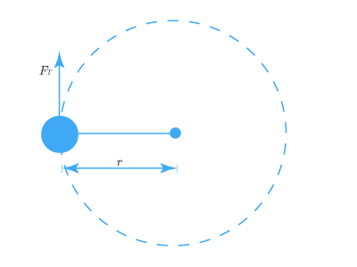
Далее система приводится во вращения, в результате действия тангенциальной силы FTFT на тело. Из второго закона Ньютона:
FT=maT или FT=m(rα)F_T = ma_T ~ или ~ F_T = m(rα)
В механике вращения крутящий момент τ=F⋅rτ = F·r занимает место силы. Умножив на rr последнее выражение, получим:
FTr=m(rα)rF_T r= m(rα) r, отсюда
τ=mr2ατ = mr^2α,
τ=Iατ = Iα
Это выражение можно использовать для определения поведения массы в ответ на действующий крутящий момент.
Момент инерции сложных фигур
Для более сложных фигур, чтобы найти момент инерции необходимо сделать несколько промежуточных вычислений. Для многих геометрических фигур существуют таблицы с уравнениями для моментов инерции. Более трудоемким будет вычисление момента инерции сложного тела, если представить его как сумму более простых тел.
Полученные моменты вращений каждого тела, объединяются в инерцию составного объекта.
Проблема, которая может возникнуть, состоит в том, что ось вращения для каждого тела будет отличаться и не будет совпадать с моментом инерции главного тела. Уравнение ниже позволяет связать момент инерции одного тела относительно момента инерции всего составного объекта:
I0=Ic+md2I_0 = I_c +md^2,
I0I_0 — момент инерции относительно точки OO (например, точка вокруг которой вращается составной главный объект), IcI_c — момент инерции относительно точки СС (например, точка вокруг которой вращается часть объекта), mm – масса части объекта, dd – расстояние между точками OO и CC.
Момент инерции важен почти во всех физических задачах, связанных с массой во вращательном движении. Он используется для расчета момента импульса и позволяет объяснить (посредством сохранения момента импульса), как изменяется вращательное движение при изменении распределения массы. А также при необходимости поиска энергии, которая хранится в виде вращательной кинетической энергии во вращающемся маховике.
Тест по теме «Момент инерции»
Когда тело продолжает двигаться при отсутствии на него воздействия каких-либо сил, говорят о проявлении инерции. Именно ею объясняются трудности удержаться на ногах при резком торможении автобуса или усидеть в седле велосипеда, когда под колеса резко выбегает кот. Кроме инерции, проявляющейся при движении тел по прямой, аналогичное явление бывает при вращении вокруг оси. В таком случае в физике говорят о моменте инерции – скалярной величине, измеряющей инертность тела при осевом вращении.
Момент инерции и его физический смысл
Обеспечить поступательное движение предмета при его толкании будет тем тяжелее, чем больше он весит. Аналогичные эксперименты предусматривались школьной программой и относились к прямо направленному действию.
Было понятно, что именно масса тела характеризует степень его инертности и является ее мерой.
При совершении предметом вращательных движений наблюдается иной вид зависимости. В данном случае мерой инертности выступает момент инерции.
Момент инерции – скалярная измеряемая характеристика инертности тела в момент совершения осевого вращения.
Задачи по определению величины момента инерции решаются с помощью теоремы Гюйгенса-Штейнера, смысл которой заключается в следующем:
МИ для тела, вращающегося вокруг какой-либо оси, равна сумме слагаемых единиц: момент инерции предмета, который вращается вокруг оси, параллельной данной, и проходящей через центр масс, а также произведения массы на расстояние между осями, возведенное в квадрат.
В приведенной формуле используются следующие обозначения: d – расстояние между осями, m – масса тела, Iz – момент инерции относительно рассматриваемой оси, а Ic – относительно оси, которая проходит через центр масс. В профильной литературе и учебниках буква I может заменяться J.
Формулировка способа количественного измерения момента инерции при осевом вращении предмета стала возможной в результате работы двух ученых-математиков: Гюйгенса и Штейнера. Теорема дает возможность быстрого решения задач на определение инерции предмета любой формы, для которого уже просчитана центробежная сила. Формула Штейнера позволяет вычислить момент инерции этого предмета относительно выбранной оси, проходящей параллельно прямой, следующей через центр фигуры.
Единицы измерения в системе СИ
Единицей измерения момента инерции, принятой в системе СИ, является кг, умноженный на метр в квадрате — кг·м². В еще одной системе измерения (СГС) единицей измерения является грамм на квадратный сантиметр — г·см².
Как рассчитать момент инерции, формула
Измерение значения момента инерции можно произвести теоретически, согласно формуле. Для этого условно движущийся предмет разбивается на мелкие составляющие, масса которых обозначается dm. В конечном итоге момент инерции (МИ) равняется сумме произведений всех образовавшихся масс на расстояние до оси, возведенное в квадрат.
Исходя из этой формулы, момент инерции, кроме массы тела, определяется положением оси, вокруг которой предмет вращается, а также его формой и габаритами.
Возможность рассчитать моменты инерции полезна, к примеру, при исследованиях свойств и структуры элементов Солнечной системы. Это так называемый безразмерный момент инерции. Высчитанная по формуле величина дает представление о распределении массы по глубине.
Виды моментов инерции
Кроме безразмерного момента инерции, в физике существуют понятия:
- центробежный МИ;
- главный МИ;
- геометрический МИ;
- МИ относительно плоскости;
- центральный МИ;
- тензор инерции;
- эллипсоид инерции.
Центробежными МИ относительно прямоугольных осей координат (декартовой системы) считаются Jxy, Jxz, Jyz. Ось ОХ является главной, когда центробежные моменты инерций Jxy и Jxz равняются нулям.
Любая точка тела может являться центром трех главных осей инерции. Они характеризуются взаимной перпендикулярностью. МИ относительно них считается главным для данного предмета. Главные оси, которые пролегают через центр масс, — являются главными центральными осями инерции предмета. МИ относительно них – главные центральные МИ. Для однородного тела ось симметрии всегда является главной центральной осью инерции.
Для геометрических МИ существуют формулы, основывающиеся на объеме относительно оси и площади относительно оси.
Твердое тело может иметь МИ относительно плоскости. Тогда это – скалярная величина, которая рассчитывается суммированием произведений массы каждой точки предмета и расстояния от нее до плоскости, возведенного в квадрат.
Понятие «Центрального МИ» связано с точкой О, МИ относительно полюса либо полярным МИ.
Момент инерции тела относительно оси вращения
МИ служит единицей измерения инерции тела, которое вращается вокруг оси, подобно тому, как масса является мерой при поступательном движении.
Определить МИ предметов касательно оси вращения позволяет формула Штейнера.
Пример:
Наглядное подтверждение применения формулы Штейнера – расчет МИ стержня, ось вращения которого проходит через конец.
Моменты инерции простейших объектов
Момент инерции некоторых однородных тел, имеющих простую форму, в зависимости от характеристик осей вращения можно определить по следующим формулам:
- МИ точечного предмета либо полого цилиндра с тонкими стенками (с массой m и радиусом r) = mr2
- МИ диска или сплошного цилиндра = 1/2 mr2
- МИ цилиндра с толстыми стенками, у которого внешний радиус обозначен r2, а внутренний – r1, :
- МИ сплошного цилиндра с осью вращения, перпендикулярной образующей цилиндра, расположенной по центру масс:
- МИ полого цилиндра с тонкими стенками и осью, перпендикулярной к цилиндру и проходящей через центр масс:
- МИ прямого тонкого стержня с осью, перпендикулярной к нему и проходящей через центр масс:
- МИ сферы с тонкими стенками и осью по центру = 2/3 mr2
- МИ шара с осью по центру = 2/5 mr2
- МИ равнобедренного треугольника с осью, перпендикулярной его плоскости и проходящей через вершину:
Примеры решения задач
Применение на практике приведенных формул происходит, например, для решения следующих задач.
Пример №1
Задано найти МИ однородного диска с известными массой и радиусом. Из дополнительных сведений: ось вращения – через центр диска.
Для решения диск разбивается на тонкие кольца, радиусы которых равняются от 0 до R. Взяв одно из них и обозначив его радиус буквой (r), а массу – (dm), формула для расчета МИ (согласно теореме Гюйгенса-Штейнера) выглядит следующим образом: (dJ=dmr2.)
С учетом подстановки в конечную формулу для определения МИ формулы для массы кольца получаем:
Пример № 2
Задано найти у того же диска МИ относительно оси, которая проходит через середину радиуса.
Из предшествующего задания используем найденную величину МИ относительно оси, которая проходит через центр масс. Используя формулу Штейнера, решаем задачу.
Если решать аналогичные задачи нет желания или времени, а контрольную работу нужно сдать в срок, на помощь придут сотрудники Феникс.Хелп.