В этой статье мы собираемся обдумать взаимосвязь энергии и длины волны вместе с примерами и решить некоторые задачи, чтобы проиллюстрировать то же самое.
Энергия находится в прямой зависимости от частоты электромагнитных излучений. Если длина волны увеличивается, это означает, что повторяемость волны будет уменьшаться, что непосредственно влияет на энергию частицы в волне.
Формула соотношения энергии и длины волны
Энергия частицы может быть связана с ее скоростью во время распространения. Скорость частицы дает представление о частоте и длине волны. Если длина волны мала, то частота и, следовательно, энергия частицы будут увеличиваться.
Если колебания частицы больше в траектории пути, то возвратность частицы в волну больше и длина волны мала, это означает, что энергия, которой обладает частица, больше.
Энергия любого тела связана с его длиной волны уравнением
E=hc/λ
Где «h» — постоянная Планка h = 6.626 * 10-34Js
C — скорость света c=3 *108 м/с и
λ — длина волны света
Энергия обратно пропорциональна длине волны света. Чем меньше длина волны, тем больше энергия частицы в волне.
Задача 1: Рассчитать энергию фотонов, испускающих красный свет. Считайте длину волны луча красного света равной 698 нм. Какова будет энергия, если длина волны уменьшится до 500 нм, то есть если источник излучает зеленый свет?
Данный:λ1=698нм
λ2=500 нм
ч = 6.626 * 10-34 Js
с=3 * 108 м/с
У нас есть,
E=hc/λ1
E = 6.626 * 10-34 Дж* 3 * 108 м/с/698* 10-9m
=0.028* 10-17=28* 10-20Дж
Энергия красной длины волны 28* 10-20Джоули.
Если длина волны λ2=500 нм
Тогда энергия, связанная с зеленым светом, равна
E=hc/λ2
E = 6.626 * 10-34 Дж* 3 * 108 м/с / 500* 10-9m
= 0.03910-17=39* 10-20Дж
Мы видим, что энергия увеличилась до 39*10-20 Джоулей при уменьшении длины волны.
Подробнее о Влияние преломления на длину волны: как, почему, подробные факты.
График взаимосвязи энергии и длины волны
По мере увеличения длины волны частота волны падает, тем самым уменьшая энергию, которой обладает волна. Если мы построим график зависимости энергии от длины волны появляющейся частицы, то график будет выглядеть так, как показано ниже.

Приведенный выше график ясно показывает, что по мере увеличения длины волны энергия, связанная с частицей, уменьшается экспоненциально.
Связь кинетической энергии и длины волны
Если скорость частицы больше, то очевидно, что кинетическая энергия частицы велика. Кинетическая энергия определяется уравнением
КЭ=1/2мВ2
Где m — масса объекта или частицы
V — скорость массы
Мы можем записать приведенное выше уравнение как
2E=мв2
Умножение «m» в обеих частях уравнения
2mE=(мВ)2
Импульс объекта определяется как произведение массы объекта на скорость, с которой он движется.
p = mv
Следовательно, приведенное выше уравнение становится
P2=2 мВ
P=√2mE
Согласно де Бройлю,
λ =h/p
Подставляя приведенное выше уравнение, мы имеем
λ =h/ √2mE
Приведенное выше уравнение дает связь между энергией и длиной волны частицы.
Подробнее о Что такое кинетическая энергия света: подробные факты.
Задача 2. Вычислить кинетическую энергию частицы массой 9.1 × 10⁻³¹ кг с длиной волны 293 нм. Кроме того, найдите скорость частицы.
Данный: λ = 293 нм
м = 9.1 × 10⁻³¹ kg
ч = 6.626 * 10-34Js
с=3 *108 м/с
У нас есть,
λ =h/ √2mE
λ2=h2/ 2мЕ
Е = ч2/ 2мλ2
=(6.626 * 10-34 Дж)2/2* 9.1* 10-31* (293*10-9) 2
= 0.28 * 10-23
Кинетическая энергия, связанная с частицей, равна 0.28*10-23 Джоули.
Теперь, чтобы вычислить скорость частицы, выведем формулу скорости из кинетической энергии:
КЕ=1/2 мВ2
2E= мв2
v=√(2Е/м)
= √(2(0.28*10-23)/(9.8*10-31))
= 0.24 * 104= 2400 м / с
Скорость частицы с длиной волны 298 нм составляет 2400 м/с.
Связь энергии электрона и длины волны
Энергия электрона определяется простым уравнением:
Е=чню
Где «h» — постоянная Планка, а
nu — частота появления электрона
Частота электрона определяется как
ню = v / λ
Где v — скорость электрона и
λ — длина волны электронной волны
Следовательно, энергия связана с длиной волны электрона как
E=hv/λ
Это соотношение позволяет найти энергию, связанную с распространением одиночного электрона с определенной длиной волны, скоростью и частотой. Энергия обратно пропорциональна длине волны. Если длина волны электрона уменьшается, энергия волны должна быть больше.

Изображение Фото: Pixabay
Получив энергию в той или иной форме, электрон переходит из более низкого энергетического состояния в более высокое энергетическое состояние. Для перехода электронов из одного состояния в другое энергия электрона определяется уравнением
Э=РE(1/нf– 1/нi)
Где RE=-2.18* 10-18m-1 является константой Ридберга
nf это конечное состояние электрона
ni это начальное состояние электрона
Мы можем далее переписать приведенное выше уравнение как
ч ню = RE(1/нf– 1/нi)
hc/λ =RE(1/нf– 1/нi)
1/λ =REhc(1/nf– 1/нi)
1/λ =R(1/nf– 1/нi)
Где,
Р=РEчс=1.097* 107
По мере того, как электрон получает энергию, электрон переходит и перескакивает в более высокое состояние энергетического уровня и высвобождает энергию электронам, присутствующим в этом состоянии, и либо становится стабильным, либо высвобождает количество энергии и возвращается в более низкие энергетические состояния.
Подробнее о 16+ Пример амплитуды волны: подробные пояснения.
Задача 3: Если электрон переходит из состояния ni=1, чтобы указать nf=2, затем рассчитайте длину волны электрона.
Данный:
ni=1
nf=2
1/λ =RE(1/нf– 1/нi)
1/λ=-1.097*107 * ( 1/2-1/1 )
1/λ=0.5485* 107
Следовательно,
λ = 1/0.5485* 107
λ =1.823*10-7
λ =182.3*10-9=182.3нм
Длина волны света, излучаемого при переходе электрона с одного энергетического уровня на другой, равна 182.3 нм.
Связь лучистой энергии и длины волны
Каждый объект поглощает световые лучи в дневное время в зависимости от его формы, размера и состава. Если температура поверхности объекта достигает температуры выше абсолютного нуля, объект будет излучать излучения в виде волн.
Это испускаемое излучение пропорционально четвертой степени абсолютной температуры объекта и определяется уравнением
U=ɛΣ Т4A
Где U — излучаемая энергия
ɛ — коэффициент излучения излучения от объекта
Σ — постоянная Стефана-Больцмана, равная Σ=5.67*10-8Вт / м2K4
T — абсолютная температура
А — площадь объекта
Объект с высокой температурой излучает излучение с короткими длинами волн, а более холодные поверхности излучают волны с большей длиной волны. В зависимости от испускаемого излучения и длины волны испускаемого излучения волны классифицируются в соответствии с приведенной ниже таблицей.
| Имя и фамилия | Радиоволны | Микроволны | Инфракрасный порт | Видимый | Ультрафиолетовое | рентген | Гамма излучение |
| Длина волны | > 1м | 1mm-1m | 700нм-1мм | 400nm-700nm | 10nm-380nm | 0.01nm-10nm | <0.01 нм |
| частота | <300 МГц | 300MHz-300GHz | 300ГГц-430ТГц | 430ТГц-750ТГц | 750ТГц-30ФГц | 30PHz-30EHz | >30 Гц |
По мере уменьшения длины волны излучения частота волны возрастает. Длина волны напрямую связана с температурой, поэтому, если частота испускаемого излучения больше, это означает, что энергия объекта высока.
Гамма-лучи, рентгеновские лучи и ультрафиолетовые лучи имеют очень короткую длину волны, поэтому энергия этих волн очень высока по сравнению с видимым, инфракрасным, микроволнами или радиоволнами. Кроме того, чем выше излучение, полученное объектом, тем больше он будет излучать в зависимости от коэффициента излучения объекта.
Ниже приведен график зависимости энергии от длины волны в секунду для разных температур. График показывает, что по мере повышения температуры системы энергия испускаемого излучения также увеличивается с температурой.

Для длины волны в видимой области эмиссия излучения максимальна. Это связано с тем, что Солнце излучает УФ-лучи вместе с инфракрасными лучами и видимыми лучами, а эти лучи представляют собой электромагнитные волны дальнего действия. Озоновый слой Земли защищает земную атмосферу от этого вредного излучения и либо отражается обратно, либо задерживается в облаках.
В видимом диапазоне в дневное время излучается больше излучений, поскольку в дневное время от Солнца поступает все больше и больше излучений, а испускается меньше ИК-лучей по сравнению с видимым спектром. Ночью температура снижается, длина волны излучения увеличивается, и объект излучает больше ИК-лучей.
Подробнее о Свойства преломления: волна, физические свойства, исчерпывающие факты.
Задача 4: Коробка длиной 11 см, шириной 2 см и воздухом 7 см нагревается до температуры 1200 Кельвинов. Если коэффициент излучения ящика равен 0.5, то рассчитайте скорость излучения энергии из ящика.
Данный:л=11см
ч=2см
б = 7cm
е =0.5
Σ=5.67* 10-8Вт / м2K4
Т=1200 К
Общая площадь ящика составляет
A=2(фунт+чб+гл)
=2(11*7+7*s 2+2*11)
=2 (77+14+22)
=0.0226 кв.м
Энергия, излучаемая коробкой, равна
U=ɛ Σ T4A
=0.5* 5.67* 10-8* 12004* 0.0226
=1328.6 Вт
Связь частоты энергии и длины волны
Чем больше частота волны, тем больше энергия, связанная с частицей. Энергия связана с частотой волны как
E=ч/ню
Где «h» — постоянная Планка.
nu — частота волны
Частота волны определяется как скорость волны в среде и длина волны.
ню = v / λ
Где v — скорость волны
λ — длина волны
Следовательно,
λ=v/ну
Это дает связь между частотой и длиной волны волны. Это говорит о том, что длина волны и частота обратно пропорциональны друг другу. Если длина волны увеличивается, частота волны уменьшится.
Подробнее о Влияние преломления на частоту: как, почему нет, подробные факты.
Задача 5. Скорость луча света, испускаемого источником, равна 1.9 × 10⁸ РС. Частота возникновения излучаемой волны составляет 450ТГц. Найдите длину волны испускаемого излучения.
Данный: v=1.9*108 м/с
F=450ТГц=450*1012Hz
Длина волны луча света равна
λ = v/f
=1.9* 108/ 450* 1012
= 0.004222 * 10-4
=422.2* 10-9=422.2нм
Луч света имеет длину волны 422.2 нм.
Связь энергии фотона и длины волны
Энергия, которой обладает фотон, называется энергией фотона и обратно пропорциональна электромагнитной волне фотона по соотношению
E=hc/λ
Где «h» — постоянная Планка.
С — скорость света
λ — длина волны фотона
Частота фотона определяется уравнением
f=с/λ
Где f — частота
Следовательно, фотон с большей длиной волны обладает небольшой единицей энергии, тогда как фотон с меньшей длиной волны дает большое количество энергии.
Подробнее о Какова длина волны фотона: как найти, несколько идей и фактов.
Задача 6: Рассчитать энергию фотона, распространяющегося в электромагнитной волне с длиной волны 620 нм.
Данный: Длина волныλ =620 нм
ч = 6.626 * 10-34 js
с=3 *108 м/с
У нас есть,
E=hc/λ
Е=6.626 * 10-34 Дж*3 * 108 м/с/620* 10-9m
= 0.032 * 10-17= 32 * 10-20 Дж
Энергия, связанная с фотоном, равна 32* 10-20Джоули.
Часто задаваемые вопросы
Q1. Вычислите длину волны электрона, движущегося со скоростью 6.35 × 10⁶ м/с
Данный: v=6.35*106м/с
м=9.1*10-31kg
ч=6.62* 10-34 Js
Кинетическая энергия электрона равна
КЕ=1/2 мВ2
=1/2 * 9.1*10-31* (6.35* 106)2
=1.83* 10-17Дж
Импульс электрона равен
P=√2mE
=√2* 9.1* 10-31* 1.83 * 10-17
= 5.7 * 10-24кг.м / с
Теперь длина волны электрона
λ =h/√2mE
= 6.62 * 10-34/ 5.7 * 10-24
= 4.8 * 10-10m
=48нм
Длина волны электрона, движущегося со скоростью 6.35*106м/с составляет 48 нм.
Q2. Черный объект площадью 180 кв.м находится при температуре 550К. Какова скорость излучения энергии от объекта?
Данный: А=180 кв.м
Т=550К
Поскольку объект имеет черный цвет, коэффициент излучения равен 1.
е =1
У нас есть,
U=ɛΣT4A
=1*с 5.67* 10-8* 5504* 180
= 0.93 * 106МОЩНОСТЬ
Мощность излучения от выброса излучения от объекта составляет 0.93*106Вт.
Какова абсолютная температура системы?
Это неизменное и совершенное значение температуры системы.
Абсолютная температура системы измеряется по шкале градусов Цельсия, Фаренгейта или Кельвина, которые измеряют ноль как абсолютный ноль градусов.
Как длина волны фотона зависит от температуры?
Температура системы определяет подвижность частиц системы.
Чем больше излучений получает система при более высоких температурах, тем больше излучения будет излучаться системой. При более высоких температурах излучаются более короткие волны, а при более низких температурах излучаются более длинные волны.
Условие задачи:
Мощность излучения лазера 100 Вт, длина волны излучения 1,2·10-6 м. Определите число фотонов, испускаемых лазером в единицу времени.
Задача №11.1.23 из «Сборника задач для подготовки к вступительным экзаменам по физике УГНТУ»
Дано:
(P=100) Вт, (lambda=1,2 cdot 10^{-6}) м, (t=1) с, (N-?)
Решение задачи:
Мощность лазера (P) – это общая энергия всех фотонов (E), которые излучаются лазером за единицу времени, поэтому справедливо записать:
[P = frac{E}{t};;;;(1)]
Очевидно, что общая энергия всех фотонов (E) равна произведению энергии одного фотона ({E_0}) на количество этих фотонов (N):
[E = N{E_0};;;;(2)]
Согласно формуле Планка, энергия фотона (E) пропорциональна частоте колебаний (nu) и определяется следующим образом:
[{E_0} = hnu ;;;;(3)]
В этой формуле (h) – это постоянная Планка, равная 6,62·10-34 Дж·с.
Известно, что частоту колебаний (nu) можно выразить через скорость света (c), которая равна 3·108 м/с, и длину волны (lambda) по следующей формуле:
[nu = frac{c}{lambda };;;;(4)]
Подставим сначала (4) в (3), полученное – в (2), и полученное после этого – в формулу (1), тогда получим:
[P = frac{{Nhc}}{{lambda t}}]
Выразим из этой формулы число фотонов (N):
[N = frac{{Plambda t}}{{hc}}]
Мы получили решение задачи в общем виде, подставим численные данные задачи в формулу и посчитаем численный ответ задачи:
[N = frac{{100 cdot 1,2 cdot {{10}^{ – 6}} cdot 1}}{{6,62 cdot {{10}^{ – 34}} cdot 3 cdot {{10}^8}}} = 6 cdot {10^{20}}]
Ответ: 6·1020.
Если Вы не поняли решение и у Вас есть какой-то вопрос или Вы нашли ошибку, то смело оставляйте ниже комментарий.
Смотрите также задачи:
11.1.22 Рубиновый лазер излучает импульс из 10^20 фотонов с длиной волны 693 нм. Длительность
11.1.24 Пучок лазерного излучения с длиной волны 3,3*10^(-7) м используется для нагревания 1 кг
11.1.25 Вычислить энергию фотона в среде с показателем преломления 1,33, если в вакууме длина
Страница 9 из 32
Рассмотрим методику определения предельной и допустимой мощностей, переносимых волнами основного и высшего типов вдоль волновода прямоугольного сечения. Мощность, переносимая волнами по волноводу, будет определяться поперечными компонентами поля. Продольные компоненты поля характеризуют лишь последовательные отражения энергии в плоскости поперечного сечения.
Поперечные компоненты поля для основной волны волновода прямоугольного сечения с учетом зависимости по времени в соответствии с формулами (2.14) и (2.15) можно записать так:

Тогда уравнение (2.94) можно переписать так:
![]()
(2.97)
Используя выражения (2.21) и (2.96), формулу (2.95) можно записать так:
![]()
(2.98)
Беря действительную часть выражений (2.97) и (2.98), получаем

(2.99)
В этих формулах Еут является максимальным значением комплексной величины Ёут, при этом аргумент Ёут принят равным нулю.

Рис. 2.26. К определению мощности, переносимой по волноводу
Плотность потока энергии в направлении оси z в произвольной точке поперечного сечения волновода в соответствии с теоремой Пойнтинга будет равна
![]()
Для определения передаваемой мощности по площади всего поперечного сечения волновода (рис. 2.26) необходимо вычислить следующий интеграл:
![]() (2.100)
(2.100)
Подставляя значение Sz, можно написать

Тогда получим следующее выражение для мощности, переносимой бегущей волной Н10:
![]() (2.101)
(2.101)
Данное выражение позволяет определить передаваемую мощность по заданной амплитуде Еут электрического поля в режиме бегущей волны. Из него же легко получить формулу для определения амплитуды напряженности электрического поля бегущей волны основного типа Еут по заданной величине передаваемой мощности Р:
![]() г(2.102)
г(2.102)
Используя формулу (2.21), выражение (2.101) можно записать следующим образом:
![]() (2.103)
(2.103)
При наличии отраженной волны мощность, передаваемая по волноводу без потерь, будет равна разности мощностей падающей и отраженной волн:

В технике волноводов часто пользуются понятиями предельной и допустимой мощностей. Предельная мощность волновода — эта такая мощность, которая может быть передана по нему без электрического пробоя. Для случая бегущей волны (КСВН-1) предельная мощность будет равна
![]()
(2.105)
где Eпред — предельная напряженность электрического поля (для воздуха при нормальных условиях равна около 30 кВ/см).
Допустимая или рабочая мощность должна быть значительно меньше предельной мощности в режиме бегущей волны. При определении допустимой мощности необходимо учитывать запас электрической прочности, так как неоднородности могут вызвать местные концентрации электрического поля и отраженные волны (значение коэффициента стоячей волны обычно допускается не более 1,5). Учитывая эти факторы, значение допустимой мощности принимают обычно не более 20—30% предельной, определяемой по формуле (2.105).
Формула (2.105) показывает, что предельная мощность, передаваемая по волноводу, изменяется в диапазоне рабочих частот. При длине волны λ=2а мощность, переносимая по волноводу, обращается в нуль.

Рис. 2.27. Изменение предельной мощности в завися мости от λ/λκρ=λ/2α
На рис. 2.27 показана зависимость предельной мощности по отношению λ/λκρ=λ/2α. На этом рисунке показана рабочая область (не заштриховано) с точки зрения передаваемой мощности. При (λ/2α)<0,5 возможно распространение высших типов волн. Поэтому предельная мощность, соответствующая λ/2α=0,5, принята за 100%. Верхней границей λ/2α принято значение, соответствующее уменьшению мощности вдвое по сравнению со значением на границе области высших типов волн. Таким образом, рабочей областью считают область
![]()
(2.106)
Для определения мощности, передаваемой в круглом волноводе, следует воспользоваться формулой (2.100). При этом необходимо взять поперечные компоненты поля. Для электрических волн типа Е поперечные компоненты поля определяются выражениями (2.51) — (2.54), а для магнитных волн типа Н — выражениями (2.57) — (2.60). Производя необходимые преобразования, для волн типа Е в круглом волноводе без потерь, включенном на согласованную нагрузку, можно получить следующую формулу полной мощности [3]:
![]()
(2.107)
где η0 — величина, обратная волновому сопротивлению среды.
Из электрических волн типа Е волна Ε01 для круглого волновода является основной. Этот тип волны аксиально симметричен, т. е. величины компонентов электрического и магнитного полей не зависят от угловой координаты φ. При волне типа Ε01 токи в стенках волновода текут только в продольном направлении, и вследствие аксиальной симметрии плотность тока одинакова во всех точках вдоль окружности. Абсолютное значение плотности тока I А/см, в стенке при переносе вдоль волновода мощности Р (в ваттах) может быть определено по формуле [4]
![]() (2.108)
(2.108)
где а — радиус волновода, см.
По волноводам круглого сечения может быть передана значительная мощность. Так, например, если принять, что электрическая прочность воздуха при нормальном атмосферном давлении составляет 30 кВ/см, то при волне типа Ε01 на 1 см2 площади поперечного сечения волновода можно пропустить мощность порядка 500 кВт при условии, что рабочая частота отстоит достаточно далеко от критической частоты и волновод нагружен на согласованную нагрузку.
Для волн типа Н полная средняя мощность, переносимая бегущей волной в круглом волноводе без потерь, определяется по формуле
![]() (2.109).
(2.109).
Волна типа Н11 является основной магнитной волной в волноводе круглого сечения. Электрическое поле волны Н11 максимально на оси волновода и равно по величине
![]() (2.110)
(2.110)
Максимальная средняя мощность, переносимая волной типа E11, выражается через Емакс формулой
![]() (2.111)
(2.111)
Полная кинетическая
энергия на единицу ширины волнового
фронта и единицу длины вдоль направления
распространения волны равна:
Ек
= ρ*а2*g/4
= Еп, (11.17.)
Еп —
потенциальная энергия.
Полная энергия на
единицу площади поверхности волны:
Е = Ек
+Еп
= ρа2g/2. (11.18.)
Кинетическая и
потенциальная энергии равны между
собой.
Выражение для
энергии на единицу ширины волнового
фронта и на единицу длины волны вдоль
направления его распространения запишем
в виде:
Еλ
= Е*λ = ρ*а2*g*λ/2. (11.19)
Но λ = 2πg/ω2,так
что
Еλ
= π*ρ*а2*g2/ω2 , (11.20.)
или, так как Т =
2π/ω
Еλ
= ρ*а2*g2*Т2/4π (11.21.)
11.6. Отбор мощности от волн.
uф
= λ/Т – фазовая скорость волны.
Выражение для
мощности, переносимой в направлении
распространения волны на единицу ширины
волнового фронта имеет вид:
Р′
=
ρ*g*a2*uф/4
= ρ*g*a2*λ/4T. (11.22.)
Мощность Р′ равна
полной энергии (кинетическая +
потенциальная) Е в волне на единицу
площади поверхности, умноженной на
величину u
= uф/2
– групповую скорость волн на глубокой
воде, с которой волны переносят энергию:
Р′= Е*u
= E*uф/2. (11.23.)
uф
= ω/к = g/ω
= g/(2πT),
k
= ω2/g,
H
= 2a.
P′
= ρ*g2*a2*T/8π
= ρ*g2*H2*T/32π.
(11.24.)
Мощность, переносимая
волнами, увеличивается прямо пропорционально
квадрату амплитуды и периоду. Именно
поэтому особенно привлекательны
длиннопериодные волны океанской зыби,
обладающие значительной амплитудой.
11.7. Утка Солтера.
Утка Солтера
является устройством, обладающим весьма
высокой эффективностью преобразования
энергии волн. Форма её обеспечивает
максимальное извлечение мощности.
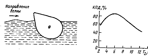
Рис. 11.7. Утка Солтера
и её эффективность. Тz
– продолжительность промежутка времени
между минимумами волн.
Волны, поступающие
слева, заставляют утку колебаться.
Цилиндрическая форма противоположной
поверхности обеспечивает отсутствие
распространения волны направо. Теряется
примерно 5% мощности волн Размер реальной
утки 10 – 15м.
11.8. Преобразование тепловой энергии океана.
В океане между
поверхностными и донными водами
достигается разность температур до
200С.
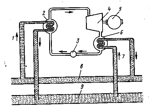
Рис. 11.8. Схема
преобразования тепловой энергии океана.
Тепловая машина использует перепад
температур между поверхностными и
глубинными водами океана. 1 – подача
тёплой воды; 2 – испаритель; 3 – насос
подачи рабочего тела; 4 – турбина; 5 –
генератор; 6 – конденсатор; 7 – подача
холодной воды;
8 – поверхность
океана; 9 – океанские глубины.
Поток тёплой воды
с объёмным расходом Q
поступает в систему при температуре Тh
= Tc
+ ΔT,
забранной с поверхности океана и покидает
её при температуре Тс
(температура холодных глубинных вод).
При определении Ро
делаем предположение об идеальном
теплообменнике. При этом ΔТ=Тh
— Тс.
Ро =
ρ*с*Q*ΔТ. (11.25.)
Механическая
мощность:
Рм
= ηк*Ро, (11.26.)
где ηк = ΔТ/Тh
— КПД идеальной машины Карно, работающей
при перепаде температур между Тh
и Тс
= Тh
– ΔT.
Идеальная
механическая выходная мощность
преобразователя тепловой энергии равна:
Рм
= (Q*c*ρ/Th)*(ΔT)2. (11.27.)
Ввиду того, что Рм
зависит от (ΔТ)2,
экономическую привлекательность имеют
районы, где ΔТ≈ 150С.
Такие районы лежат в тропиках.
Теплообменники
передают тепло от одной жидкости к
другой, не позволяя им смешиваться. В
таком теплообменнике поток воды движется
по трубам, омываемом рабочим телом.
Основные неприятности возникают из-за
низкой теплопроводности самой морской
воды. Для преодоления всех термических
сопротивлений при теплопередаче
необходим определённый перепад температур
σТ.
Пусть Рвф
– тепловой поток от морской воды (в) к
рабочему телу жидкости
(ф). Тогда
Рвф
= σT/Rвф (11.28.)
где Rвф
– сопротивление теплопередаче от воды
к рабочему телу.
Аналогичное падение
температуры σТ будет наблюдаться и во
втором теплообменнике при передаче
тепла от рабочего тела к морской воде,
то действительный перепад температур,
приводящий в действие тепловую машину,
будет равен не ΔТ, а
Rвф
(в)
Δ2Т
= ΔТ — 2σТ. (11.29.)
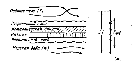
Рис. 11.9. Кожухотрубный
теплообменник.
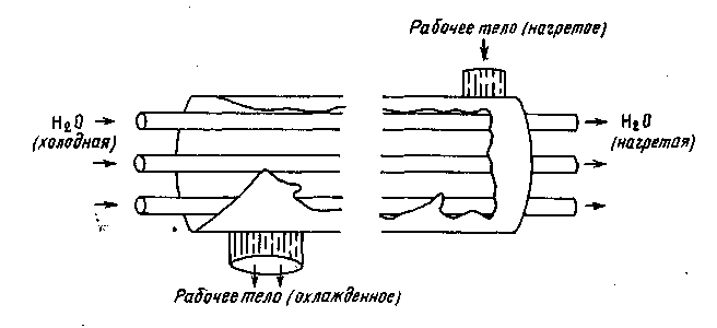
Рис. 11.10. Сопротивление
теплопередаче через стенку теплообменника.
Для идеальной
тепловой машины Карно выходная мощность
равна:
Р2
= [(ΔТ — 2σТ)/Тh]*(σT/Rвф). (11.30.)
Трубы теплообменника
должны быть сделаны из, хорошо проводящего
тепло, металла и их должно быть достаточно
много, чтобы они могли обеспечить
необходимую площадь рабочей поверхности.
Полное термическое сопротивление можно
выразить через удельное термическое
сопротивление rвф
и общую площадь стенок Авф^
Rвф
= rвф/Aвф. (11.31.)
Необходимый расход
воды через теплообменник определяется
отбираемой от него мощностью, теплопередачей
и абсолютными значениями температур.
Мощность, отдаваемая
горячей водой, равна:
Рhв=
ρ*c*Q*(Thвin
— Thвout). (11.32/)
при падении
температуры
Тhвin
— Thвout
= ΔT
– 2σT. (11.33.)
Внутренние
поверхности трубок теплообменников
уязвимы для оседания морских организмов,
что увеличивает сопротивление
теплопередаче. Биообрастание – одна
из главных проблем при проектировании
таких станций.
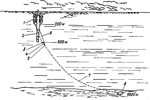
Рис. 11.11. Подводная
платформа для ОТЭС электрической
мощностью 400 МВт. Платформа может быть
установлена на якоре при любой глубине
моря. 1 – платформа; 2 – трубопровод
холодной воды; 3 – распорка; 4 — бридель;
5 – шарнир; 6 – трапеция; 7 – якорный
трос; 8 – якорь.
В качестве рабочего
тела аммиак, фреоны или воду. При
использовании воды, её температуру
кипения необходимо понизить до температуры
поверхностных вод за счёт вакуумирования.
Соседние файлы в предмете [НЕСОРТИРОВАННОЕ]
- #
- #
- #
- #
- #
- #
- #
- #
- #
- #
- #
This article is about transport and capture of energy in ocean waves. For other aspects of waves in the ocean, see Wind wave. For other uses of wave or waves, see Wave (disambiguation).
Wave power is the capture of energy of wind waves to do useful work – for example, electricity generation, water desalination, or pumping water. A machine that exploits wave power is a wave energy converter (WEC).
Waves are generated by wind passing over the sea’s surface. As long as the waves propagate slower than the wind speed just above, energy is transferred from the wind to the waves. Air pressure differences between the windward and leeward sides of a wave crest and surface friction from the wind cause shear stress and wave growth.[1]
Wave power is distinct from tidal power, which captures the energy of the current caused by the gravitational pull of the Sun and Moon. Other forces can create currents, including breaking waves, wind, the Coriolis effect, cabbeling, and temperature and salinity differences.
As of 2022, wave power is not widely employed for commercial applications, after a long series of trial projects. Attempts to use this energy began in 1890 or earlier,[2] mainly due to its high power density. Just below the ocean’s water surface the wave energy flow, in time-average, is typically five times denser than the wind energy flow 20 m above the sea surface, and 10 to 30 times denser than the solar energy flow.[3]
In 2000 the world’s first commercial wave power device, the Islay LIMPET was installed on the coast of Islay in Scotland and connected to the UK national grid.[4] In 2008, the first experimental multi-generator wave farm was opened in Portugal at the Aguçadoura wave park.[5] Both projects have since ended.
Wave energy converters can be classified based on their working principle as either:[6][7]
- oscillating water columns (with air turbine)
- oscillating bodies (with hydroelectric motor, hydraulic turbine, linear electrical generator)
- overtopping devices (with low-head hydraulic turbine)
History[edit]
The first known patent to extract energy from ocean waves was in 1799, filed in Paris by Pierre-Simon Girard and his son.[8] An early device was constructed around 1910 by Bochaux-Praceique to power his house in Royan, France.[9] It appears that this was the first oscillating water-column type of wave-energy device.[10] From 1855 to 1973 there were 340 patents filed in the UK alone.[8]
Modern pursuit of wave energy was pioneered by Yoshio Masuda’s 1940s experiments.[11] He tested various concepts, constructing hundreds of units used to power navigation lights. Among these was the concept of extracting power from the angular motion at the joints of an articulated raft, which Masuda proposed in the 1950s.[12]
The oil crisis in 1973 renewed interest in wave energy. Substantial wave-energy development programmes were launched by governments in several countries, in particular in the UK, Norway and Sweden.[3] Researchers re-examined waves’ potential to extract energy, notably Stephen Salter, Johannes Falnes, Kjell Budal, Michael E. McCormick, David Evans, Michael French, Nick Newman, and C. C. Mei.
Salter’s 1974 invention became known as Salter’s duck or nodding duck, officially the Edinburgh Duck. In small scale tests, the Duck’s curved cam-like body can stop 90% of wave motion and can convert 90% of that to electricity, giving 81% efficiency.[13] In the 1980s, several other first-generation prototypes were tested, but as oil prices ebbed, wave-energy funding shrank. Climate change later reenergized the field.[14][3]
The world’s first wave energy test facility was established in Orkney, Scotland in 2003 to kick-start the development of a wave and tidal energy industry. The European Marine Energy Centre(EMEC) has supported the deployment of more wave and tidal energy devices than any other single site.[15] Subsequent to its establishment test facilities occurred also in many other countries around the world, providing services and infrastructure for device testing.[16]
The £10 million Saltire prize challenge was to be awarded to the first to be able to generate 100 GWh from wave power over a continuous two-year period by 2017 (about 5.7 MW average).[17] The prize was never awarded. A 2017 study by Strathclyde University and Imperial College focused on the failure to develop «market ready» wave energy devices – despite a UK government investment of over £200 million over 15 years.[18]
Public bodies have continued and in many countries stepped up the research and development funding for wave energy during the 2010s. This includes both EU, US and UK where the annual allocation has typically been in the range 5-50 million USD.[19][20][21][22][23] Combined with private funding, this has led to a large number of ongoing wave energy projects (see List of wave power projects).
Physical concepts[edit]
Like most fluid motion, the interaction between ocean waves and energy converters is a high-order nonlinear phenomenon. It is described using the incompressible Navier-Stokes equations

where  is the fluid velocity,
  is the pressure,
  the density,
  the viscosity, and
  the net external force on each fluid particle (typically gravity). Under typical conditions, however, the movement of waves is described by Airy wave theory, which posits that
- fluid motion is roughly irrotational,
- pressure is approximately constant at the water surface, and
- the seabed depth is approximately constant.
In situations relevant for energy harvesting from ocean waves these assumptions are usually valid.
Airy equations[edit]
The first condition implies that the motion can be described by a velocity potential  :[24]
:[24]

which must satisfy the Laplace equation,

In an ideal flow, the viscosity is negligible and the only external force acting on the fluid is the earth gravity  . In those circumstances, the Navier-Stokes equations reduces to

which integrates (spatially) to the Bernoulli conservation law:

Linear potential flow theory[edit]

Motion of a particle in an ocean wave.
A = At deep water. The circular motion magnitude of fluid particles decreases exponentially with increasing depth below the surface.
B = At shallow water (ocean floor is now at B). The elliptical movement of a fluid particle flattens with decreasing depth.
1 = Propagation direction.
2 = Wave crest.
3 = Wave trough.
When considering small amplitude waves and motions, the quadratic term  can be neglected, giving the linear Bernoulli equation,

and third Airy assumptions then imply

These constraints entirely determine sinusoidal wave solutions of the form

where  determines the wavenumber of the solution and
  and
and  are determined by the boundary constraints (and ). Specifically,

The surface elevation  can then be simply derived as

a plane wave progressing along the x-axis direction.
Consequences[edit]
Oscillatory motion is highest at the surface and diminishes exponentially with depth. However, for standing waves (clapotis) near a reflecting coast, wave energy is also present as pressure oscillations at great depth, producing microseisms.[1] Pressure fluctuations at greater depth are too small to be interesting for wave power conversion.
The behavior of Airy waves offers two interesting regimes: water deeper than half the wavelength, as is common in the sea and ocean, and shallow water, with wavelengths larger than about twenty times the water depth. Deep waves are dispersionful: Waves of long wavelengths propagate faster and tend to outpace those with shorter wavelengths. Deep-water group velocity is half the phase velocity. Shallow water waves are dispersionless: group velocity is equal to phase velocity, and wavetrains propagate undisturbed.[1][25][26]
The following table summarizes the behavior of waves in the various regimes:
| quantity | symbol | units | deep water (h > 1⁄2 λ) |
shallow water (h < 0.05 λ) |
intermediate depth (all λ and h) |
|---|---|---|---|---|---|
| phase velocity | 
|
m / s | 
|

|

|
| group velocity[a] | 
|
m / s | 
|
|

|
| ratio | 
|
– | 
|

|

|
| wavelength | 
|
m | 
|

|
for given period T, the solution of:
|
| general | |||||
| wave energy density | 
|
J / m2 | 
|
||
| wave energy flux | 
|
W / m | 
|
||
| angular frequency |
|
rad / s | 
|
||
| wavenumber |
|
rad / m | 
|

Wave power formula[edit]

Photograph of the elliptical trajectories of water particles under a – progressive and periodic – surface gravity wave in a wave flume. The wave conditions are: mean water depth d = 2.50 ft (0.76 m), wave height H = 0.339 ft (0.103 m), wavelength λ = 6.42 ft (1.96 m), period T = 1.12 s.[27]
In deep water where the water depth is larger than half the wavelength, the wave energy flux is[b]

with P the wave energy flux per unit of wave-crest length, Hm0 the significant wave height, Te the wave energy period, ρ the water density and g the acceleration by gravity. The above formula states that wave power is proportional to the wave energy period and to the square of the wave height. When the significant wave height is given in metres, and the wave period in seconds, the result is the wave power in kilowatts (kW) per metre of wavefront length.[28][29][30][31]
For example, consider moderate ocean swells, in deep water, a few km off a coastline, with a wave height of 3 m and a wave energy period of 8 s. Solving for power produces

or 36 kilowatts of power potential per meter of wave crest.
In major storms, the largest offshore sea states have significant wave height of about 15 meters and energy period of about 15 seconds. According to the above formula, such waves carry about 1.7 MW of power across each meter of wavefront.
An effective wave power device captures a significant portion of the wave energy flux. As a result, wave heights diminish in the region behind the device.
Energy and energy flux[edit]
In a sea state, the mean energy density per unit area of gravity waves on the water surface is proportional to the wave height squared, according to linear wave theory:[1][26]
 [c][32]

where E is the mean wave energy density per unit horizontal area (J/m2), the sum of kinetic and potential energy density per unit horizontal area. The potential energy density is equal to the kinetic energy,[1] both contributing half to the wave energy density E, as can be expected from the equipartition theorem.
The waves propagate on the surface, where crests travel with the phase velocity while the energy is transported horizontally with the group velocity. The mean transport rate of the wave energy through a vertical plane of unit width, parallel to a wave crest, is the energy flux (or wave power, not to be confused with the output produced by a device), and is equal to:[33][1]
- with cg the group velocity (m/s).

Due to the dispersion relation for waves under gravity, the group velocity depends on the wavelength λ, or equivalently, on the wave period T.
Wave height is determined by wind speed, the length of time the wind has been blowing, fetch (the distance over which the wind excites the waves) and by the bathymetry (which can focus or disperse the energy of the waves). A given wind speed has a matching practical limit over which time or distance do not increase wave size. At this limit the waves are said to be «fully developed». In general, larger waves are more powerful but wave power is also determined by wavelength, water density, water depth and acceleration of gravity.
Wave energy converters[edit]
Wave energy converters (WECs) are generally categorized by the method, by location and by the power take-off system. Locations are shoreline, nearshore and offshore. Types of power take-off include: hydraulic ram, elastomeric hose pump, pump-to-shore, hydroelectric turbine, air turbine,[34] and linear electrical generator.

Different conversion routes from wave energy to useful energy in terms or electricity or direct use.
The four most common approaches are:
- point absorber buoys
- surface attenuators
- oscillating water columns
- overtopping devices

Generic wave energy concepts: 1. Point absorber, 2. Attenuator, 3. Oscillating wave surge converter, 4. Oscillating water column, 5. Overtopping device, 6. Submerged pressure differential, 7. Floating in-air converters.
Point absorber buoy[edit]
This device floats on the surface, held in place by cables connected to the seabed. The point-absorber has a device width much smaller than the incoming wavelength λ. Energy is absorbed by radiating a wave with destructive interference to the incoming waves. Buoys use the swells’ rise and fall to generate electricity directly via linear generators,[35] generators driven by mechanical linear-to-rotary converters,[36] or hydraulic pumps.[37] Energy extracted from waves may affect the shoreline, implying that sites should remain well offshore.[38]
Surface attenuator[edit]
These devices use multiple floating segments connected to one another. They are oriented perpendicular to incoming waves. A flexing motion is created by swells, and that motion drives hydraulic pumps to generate electricity.
Oscillating wave surge converter[edit]
These devices typically have one end fixed to a structure or the seabed while the other end is free to move. Energy is collected from the relative motion of the body compared to the fixed point. Converters often come in the form of floats, flaps, or membranes. Some designs incorporate parabolic reflectors to focus energy at the point of capture. These systems capture energy from the rise and fall of waves.[39]
Oscillating water column[edit]
Oscillating water column devices can be located onshore or offshore. Swells compress air in an internal chamber, forcing air through a turbine to create electricity.[40] Significant noise is produced as air flows through the turbines, potentially affecting nearby birds and marine organisms. Marine life could possibly become trapped or entangled within the air chamber.[38] It draws energy from the entire water column.[41]
Overtopping device[edit]
Overtopping devices are long structures that use wave velocity to fill a reservoir to a greater water level than the surrounding ocean. The potential energy in the reservoir height is captured with low-head turbines. Devices can be on- or offshore.
Submerged pressure differential[edit]
Submerged pressure differential based converters[42] use flexible (typically reinforced rubber) membranes to extract wave energy. These converters use the difference in pressure at different locations below a wave to produce a pressure difference within a closed power take-off hydraulic system. This pressure difference is usually used to produce flow, which drives a turbine and electrical generator. Submerged pressure differential converters typically use flexible membranes as the working surface between the water and the power take-off. Membranes are pliant and low mass, which can strengthen coupling with the wave’s energy. Their pliancy allows large changes in the geometry of the working surface, which can be used to tune the converter for specific wave conditions and to protect it from excessive loads in extreme conditions.
A submerged converter may be positioned either on the seafloor or in midwater. In both cases, the converter is protected from water impact loads which can occur at the free surface. Wave loads also diminish in non-linear proportion to the distance below the free surface. This means that by optimizing depth, protection from extreme loads and access to wave energy can be balanced.
Floating in-air converters[edit]

Wave Power Station using a pneumatic Chamber

Simplified design of Wave Power Station
Floating in-air converters potentially offer increased reliability because the device is located above the water, which also eases inspection and maintenance. Examples of different concepts of floating in-air converters include:
- roll damping energy extraction systems with turbines in compartments containing sloshing water
- horizontal axis pendulum systems
- vertical axis pendulum systems
Environmental effects[edit]
Common environmental concerns associated with marine energy include:[43][38]
- The effects of electromagnetic fields and underwater noise;
- Physical presence’s potential to alter the behavior of marine mammals, fish, and seabirds with attraction, avoidance, entanglement
- Potential effect on marine processes such as sediment transport and water quality.
- Foundation/mooring systems can affect benthic organisms via entanglement/entrapment
- Electromotive force effects produced from subsea power cables.
- Minor collision risk
- Artificial reef accumulation near fixed installations
- Potential disuption to roosting sites
Potential[edit]
Wave energy’s worldwide theoretical potential has been estimated to be greater than 2 TW.[44] Locations with the most potential for wave power include the western seaboard of Europe, the northern coast of the UK, and the Pacific coastlines of North and South America, Southern Africa, Australia, and New Zealand. The north and south temperate zones have the best sites for capturing wave power. The prevailing westerlies in these zones blow strongest in winter.
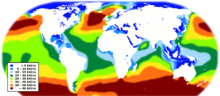
World wave energy resource map
The National Renewable Energy Laboratory (NREL) estimated the theoretical wave energy potential for various countries. It estimated that the US’ potential was equivalent to 1170 TWh per year or almost 1/3 of the country’s electricity consumption.[45] The Alaska coastline accounted for ~50% of the total.
Note that the technical and economical potential will be lower than the given values for the theoretical potential.[46][47]
Challenges[edit]
|
This section needs expansion with: what are the main technical difficulties?. You can help by adding to it. (February 2023) |
Environmental impacts must be addressed.[30][48] Socio-economic challenges include the displacement of commercial and recreational fishermen, and may present navigation hazards.[49] Supporting infrastructure, such as grid connections, must be provided.[50] Commercial WECs have not always been successful. In 2019, for example, Seabased Industries AB in Sweden was liquidated due to «extensive challenges in recent years, both practical and financial».[51]
Current wave power generation technology is subject to many technical limitations.[52] These limitations stem from the complex and dynamic nature of ocean waves, which require robust and efficient technology to capture the energy. Challenges include designing and building wave energy devices that can withstand the corrosive effects of saltwater, harsh weather conditions, and extreme wave forces.[53] Additionally, optimizing the performance and efficiency of wave energy converters, such as oscillating water column (OWC) devices, point absorbers, and overtopping devices, requires overcoming engineering complexities related to the dynamic and variable nature of waves.[54] Furthermore, developing effective mooring and anchoring systems to keep wave energy devices in place in the harsh ocean environment, and developing reliable and efficient power take-off mechanisms to convert the captured wave energy into electricity, are also technical challenges in wave power generation.[55]
Wave farms[edit]
A wave farm (wave power farm or wave energy park) is a group of colocated wave energy devices. The devices interact hydrodynamically and electrically, according to the number of machines, spacing and layout, wave climate, coastal and benthic geometry, and control strategies. The design process is a multi-optimization problem seeking high power production, low costs and limited power fluctuations.[56]
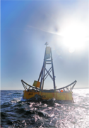
Gallery of wave energy installations[edit]
-

-

Azura at the US Navy’s Wave Energy Test Site (WETS) on Oahu.
-

The AMOG Wave Energy Converter (WEC), in operation off SW England (2019).
-

The mWave converter by Bombora Wave Power.
-

CalWave Power Technologies, Inc. wave energy converter in California.


Patents[edit]
- WIPO patent application WO2016032360 — 2016 Pumped-storage system – «Pressure buffering hydro power» patent application
- U.S. Patent 8,806,865 — 2011 Ocean wave energy harnessing device – Pelamis/Salter’s Duck Hybrid patent
- U.S. Patent 3,928,967 — 1974 Apparatus and method of extracting wave energy – The original «Salter’s Duck» patent
- U.S. Patent 4,134,023 — 1977 Apparatus for use in the extraction of energy from waves on water – Salter’s method for improving «duck» efficiency
- U.S. Patent 6,194,815 — 1999 Piezoelectric rotary electrical energy generator
- U.S. Patent 1,930,958 — 1932 Wave Motor — Parsons Ocean Power Plant — Herring Cove Nova Scotia — March 1925. The world’s first commercial plant to convert ocean wave energy into electrical power. Designer — Osborne Havelock Parsons — born in 1873 Petitcodiac, New Brunswick.
- Wave energy converters utilizing pressure differences US 20040217597 A1 — 2004 Wave energy converters utilizing pressure differences[57]
A UK-based company has developed a Waveline Magnet that can achieve a levelized cost of electricity of £0.01/kWh with minimal levels of maintenance.[58]
See also[edit]
- List of wave power stations
- List of wave power projects
- Wave power in Australia
- Wave power in New Zealand
- Wave power in Scotland
- Wave power in the United States
- Marine energy
- Ocean thermal energy conversion
- Office of Energy Efficiency and Renewable Energy (OEERE)
- World energy consumption
Notes[edit]
- ^ For determining the group velocity the angular frequency ω is considered as a function of the wavenumber k, or equivalently, the period T as a function of the wavelength λ.
- ^ The energy flux is with the group velocity, see Herbich, John B. (2000). Handbook of coastal engineering. McGraw-Hill Professional. A.117, Eq. (12). ISBN 978-0-07-134402-9. The group velocity is , see the collapsed table «Properties of gravity waves on the surface of deep water, shallow water and at intermediate depth, according to linear wave theory» in the section «Wave energy and wave energy flux» below.
- ^ Here, the factor for random waves is 1⁄16, as opposed to 1⁄8 for periodic waves – as explained hereafter. For a small-amplitude sinusoidal wave with wave amplitude the wave energy density per unit horizontal area is or using the wave height for sinusoidal waves. In terms of the variance of the surface elevation the energy density is . Turning to random waves, the last formulation of the wave energy equation in terms of is also valid (Holthuijsen, 2007, p. 40), due to Parseval’s theorem. Further, the significant wave height is defined as , leading to the factor 1⁄16 in the wave energy density per unit horizontal area.


References[edit]
- ^ a b c d e f Phillips, O.M. (1977). The dynamics of the upper ocean (2nd ed.). Cambridge University Press. ISBN 978-0-521-29801-8.
- ^ Christine Miller (August 2004). «Wave and Tidal Energy Experiments in San Francisco and Santa Cruz». Archived from the original on October 2, 2008. Retrieved August 16, 2008.
- ^ a b c «Wave energy and its utilization». Slideshare. June 1, 1999. Retrieved April 28, 2023.
- ^ «World’s first commercial wave power station activated in Scotland». Archived from the original on August 5, 2018. Retrieved June 5, 2018.
- ^ Joao Lima. Babcock, EDP and Efacec to Collaborate on Wave Energy projects Archived September 24, 2015, at the Wayback Machine Bloomberg, September 23, 2008.
- ^ Falcão, António F. de O. (April 1, 2010). «Wave energy utilization: A review of the technologies». Renewable and Sustainable Energy Reviews. 14 (3): 899–918. doi:10.1016/j.rser.2009.11.003. ISSN 1364-0321.
- ^ Madan, D.; Rathnakumar, P.; Marichamy, S.; Ganesan, P.; Vinothbabu, K.; Stalin, B. (October 21, 2020), «A Technological Assessment of the Ocean Wave Energy Converters», Lecture Notes in Mechanical Engineering, Singapore: Springer Singapore, pp. 1057–1072, doi:10.1007/978-981-15-4739-3_91, ISBN 978-981-15-4738-6, S2CID 226322561, retrieved June 2, 2022
- ^ a b Clément; et al. (2002). «Wave energy in Europe: current status and perspectives». Renewable and Sustainable Energy Reviews. 6 (5): 405–431. doi:10.1016/S1364-0321(02)00009-6.
- ^ «The Development of Wave Power» (PDF). Archived from the original (PDF) on July 27, 2011. Retrieved December 18, 2009.
- ^ Morris-Thomas; Irvin, Rohan J.; Thiagarajan, Krish P.; et al. (2007). «An Investigation Into the Hydrodynamic Efficiency of an Oscillating Water Column». Journal of Offshore Mechanics and Arctic Engineering. 129 (4): 273–278. doi:10.1115/1.2426992.
- ^ «Wave Energy Research and Development at JAMSTEC». Archived from the original on July 1, 2008. Retrieved December 18, 2009.
- ^ Farley, F. J. M. & Rainey, R. C. T. (2006). «Radical design options for wave-profiling wave energy converters» (PDF). International Workshop on Water Waves and Floating Bodies. Loughborough. Archived (PDF) from the original on July 26, 2011. Retrieved December 18, 2009.
- ^ «Edinburgh Wave Energy Project» (PDF). University of Edinburgh. Archived from the original (PDF) on October 1, 2006. Retrieved October 22, 2008.
- ^ Falnes, J. (2007). «A review of wave-energy extraction». Marine Structures. 20 (4): 185–201. doi:10.1016/j.marstruc.2007.09.001.
- ^ «Our history». Retrieved April 28, 2023.
- ^ Aderinto, Tunde and Li, Hua (2019). «Review on power performance and efficiency of wave energy converters». Energie. 12 (22). doi:10.3390/en12224329.
{{cite journal}}: CS1 maint: multiple names: authors list (link) - ^ «Ocean Energy Teams Compete for $16 Million Scotland Prize». National geographic. September 7, 2012.
- ^ Scott Macnab (November 2, 2017). «Government’s £200m wave energy plan undermined by failures». The Scotsman. Archived from the original on December 5, 2017. Retrieved December 5, 2017.
- ^ Wave Energy Bill Approved by U.S. House Science Committee http://www.renewableenergyworld.com/articles/2007/06/wave-energy-bill-approved-by-u-s-house-science-committee-48984.html June 18, 2007
- ^ DOE announces first marine renewable energy grants http://uaelp.pennnet.com/Articles/Article_Display.cfm?Section=ONART&PUBLICATION_ID=22&ARTICLE_ID=341078&C=ENVIR&dcmp=rss Archived 2004-07-27 at the Wayback Machine September 30, 2008
- ^ «Ocean energy». Retrieved April 28, 2023.
- ^ «Projects to unlock the potential of marine wave energy». Retrieved April 28, 2023.
- ^ «Wave energy Scotland». Retrieved April 28, 2023.
- ^ Numerical modelling of wave energy converters : state-of-the-art techniques for single devices and arrays. Matt Folley. London, UK. 2016. ISBN 978-0-12-803211-4. OCLC 952708484.
{{cite book}}: CS1 maint: others (link) - ^ R. G. Dean & R. A. Dalrymple (1991). Water wave mechanics for engineers and scientists. Advanced Series on Ocean Engineering. Vol. 2. World Scientific, Singapore. ISBN 978-981-02-0420-4. See page 64–65.
- ^ a b Goda, Y. (2000). Random Seas and Design of Maritime Structures. World Scientific. ISBN 978-981-02-3256-6.
- ^ Figure 6 from: Wiegel, R.L.; Johnson, J.W. (1950), «Elements of wave theory», Proceedings 1st International Conference on Coastal Engineering, Long Beach, California: ASCE, pp. 5–21
- ^ Tucker, M.J.; Pitt, E.G. (2001). «2». In Bhattacharyya, R.; McCormick, M.E. (eds.). Waves in ocean engineering (1st ed.). Oxford: Elsevier. pp. 35–36. ISBN 978-0080435664.
- ^ «Wave Power». University of Strathclyde. Archived from the original on December 26, 2008. Retrieved November 2, 2008.
- ^ a b «Wave Energy Potential on the U.S. Outer Continental Shelf» (PDF). United States Department of the Interior. Archived from the original (PDF) on July 11, 2009. Retrieved October 17, 2008.
- ^ Academic Study: Matching Renewable Electricity Generation with Demand: Full Report Archived November 14, 2011, at the Wayback Machine. Scotland.gov.uk.
- ^ Holthuijsen, Leo H. (2007). Waves in oceanic and coastal waters. Cambridge: Cambridge University Press. ISBN 978-0-521-86028-4.
- ^ Reynolds, O. (1877). «On the rate of progression of groups of waves and the rate at which energy is transmitted by waves». Nature. 16 (408): 343–44. Bibcode:1877Natur..16R.341.. doi:10.1038/016341c0.
Lord Rayleigh (J. W. Strutt) (1877). «On progressive waves». Proceedings of the London Mathematical Society. 9 (1): 21–26. doi:10.1112/plms/s1-9.1.21. Reprinted as Appendix in: Theory of Sound 1, MacMillan, 2nd revised edition, 1894. - ^ Embedded Shoreline Devices and Uses as Power Generation Sources Kimball, Kelly, November 2003
- ^ «Seabased AB wave energy technology». Archived from the original on October 10, 2017. Retrieved October 10, 2017.
- ^ «PowerBuoy Technology — Ocean Power Technologies». Archived from the original on October 10, 2017. Retrieved October 10, 2017.
- ^ «Perth Wave Energy Project – Carnegie’s CETO Wave Energy technology». Archived from the original on October 11, 2017. Retrieved October 10, 2017.
- ^ a b c «Tethys». Archived from the original on May 20, 2014. Retrieved April 21, 2014.
- ^ McCormick, Michael E.; Ertekin, R. Cengiz (2009). «Renewable sea power: Waves, tides, and thermals – new research funding seeks to put them to work for us». Mechanical Engineering. ASME. 131 (5): 36–39. doi:10.1115/1.2009-MAY-4.
- ^ «Extracting Energy From Ocean Waves». Archived from the original on August 15, 2015. Retrieved April 23, 2015.
- ^ Blain, Loz (August 1, 2022). «Blowhole wave energy generator exceeds expectations in 12-month test». New Atlas. Retrieved August 8, 2022.
- ^ Kurniawan, Adi; Greaves, Deborah; Chaplin, John (December 8, 2014). «Wave energy devices with compressible volumes». Proceedings of the Royal Society of London A: Mathematical, Physical and Engineering Sciences. 470 (2172): 20140559. Bibcode:2014RSPSA.47040559K. doi:10.1098/rspa.2014.0559. ISSN 1364-5021. PMC 4241014. PMID 25484609.
- ^ «Tethys». Archived from the original on November 10, 2014.
- ^ Gunn, Kester; Stock-Williams, Clym (August 2012). «Quantifying the global wave power resource». Renewable Energy. Elsevier. 44: 296–304. doi:10.1016/j.renene.2012.01.101.
- ^ «Ocean Wave Energy | BOEM». www.boem.gov. Archived from the original on March 26, 2019. Retrieved March 10, 2019.
- ^ «Renewable Energy Economic Potential». www.nrel.gov. Retrieved May 2, 2023.
- ^ Teske, S.; Nagrath, K.; Morris, T.; Dooley, K. (2019). «Renewable Energy Resource Assessment». In Teske, S. (ed.). Achieving the Paris Climate Agreement Goals. Springer. doi:10.1007/978-3-030-05843-2_7.
- ^ Marine Renewable Energy Programme Archived August 3, 2011, at the Wayback Machine, NERC Retrieved August 1, 2011
- ^ Steven Hackett:Economic and Social Considerations for Wave Energy Development in California CEC Report Nov 2008 Archived May 26, 2009, at the Wayback Machine Ch2, pp22-44 California Energy Commission|Retrieved December 14, 2008
- ^ Gallucci, M. (December 2019). «At last, wave energy tech plugs into the grid — [News]». IEEE Spectrum. 56 (12): 8–9. doi:10.1109/MSPEC.2019.8913821. ISSN 1939-9340.
- ^ «Seabased Closes Production Facility in Sweden». marineenergy.biz. January 2019. Retrieved December 12, 2019.
- ^ Singh, Rajesh; Kumar, Suresh; Gehlot, Anita; Pachauri, Rupendra (February 2018). «An imperative role of sun trackers in photovoltaic technology: A review». Renewable and Sustainable Energy Reviews. 82: 3263–3278. doi:10.1016/j.rser.2017.10.018.
- ^ Felix, Angélica; V. Hernández-Fontes, Jassiel; Lithgow, Débora; Mendoza, Edgar; Posada, Gregorio; Ring, Michael; Silva, Rodolfo (July 2019). «Wave Energy in Tropical Regions: Deployment Challenges, Environmental and Social Perspectives». Journal of Marine Science and Engineering. 7 (7): 219. doi:10.3390/jmse7070219. ISSN 2077-1312.
- ^ Xamán, J.; Rodriguez-Ake, A.; Zavala-Guillén, I.; Hernández-Pérez, I.; Arce, J.; Sauceda, D. (April 2020). «Thermal performance analysis of a roof with a PCM-layer under Mexican weather conditions». Renewable Energy. 149: 773–785. doi:10.1016/j.renene.2019.12.084.
- ^ Røe, Oluf Dimitri; Stella, Giulia Maria (2017), Testa, Joseph R. (ed.), «Malignant Pleural Mesothelioma: History, Controversy, and Future of a Man-Made Epidemic», Asbestos and Mesothelioma, Cham: Springer International Publishing, pp. 73–101, doi:10.1007/978-3-319-53560-9_4, ISBN 978-3-319-53558-6, retrieved April 18, 2023
- ^ Giassi, Marianna; Göteman, Malin (April 2018). «Layout design of wave energy parks by a genetic algorithm». Ocean Engineering. 154: 252–261. doi:10.1016/j.oceaneng.2018.01.096. ISSN 0029-8018. S2CID 96429721.
- ^ FreePatentsOnline.com Wave energy converters utilizing pressure differences Archived October 31, 2014, at the Wayback Machine, April 11, 2004
- ^ «Wave magnets offer ‘cheapest clean energy ever’«. The Independent. August 31, 2022.
Further reading[edit]
- Cruz, Joao (2008). Ocean Wave Energy – Current Status and Future Prospects. Springer. ISBN 978-3-540-74894-6., 431 pp.
- Falnes, Johannes (2002). Ocean Waves and Oscillating Systems. Cambridge University Press. ISBN 978-0-521-01749-7., 288 pp.
- McCormick, Michael (2007). Ocean Wave Energy Conversion. Dover. ISBN 978-0-486-46245-5., 256 pp.
- Twidell, John; Weir, Anthony D.; Weir, Tony (2006). Renewable Energy Resources. Taylor & Francis. ISBN 978-0-419-25330-3., 601 pp.
External links[edit]
![]()
Wikimedia Commons has media related to Wave power.
- Kate Galbraith (September 22, 2008). «Power From the Restless Sea Stirs the Imagination». The New York Times. Retrieved October 9, 2008.
- «Wave Power: The Coming Wave» from the Economist, June 5, 2008
- Tethys – the Tethys database from the Pacific Northwest National Laboratory
- Wave Swell Energy video on YouTube