Как найти норму числа

Вычисление нормы и чисел обусловленности матрицы

1
норма матрицы представляет из себя
максимальное из чисел, полученных при
сложении всех элементов каждого столбца,
взятых по модулю. Не путайте со сложением
матриц!

Р
ассмотрим
на примере: пусть дана матрица размера
3х2. В первом столбце стоят элементы: 8,
3, 8. Все элементы положительные. Найдем
их сумму: 8+3+8=19. В втором столбце стоят
элементы: 8, -2, -8. Два элемента — отрицательные,
поэтому при сложении этих чисел,
необходимо подставлять модуль этих
чисел (т.е. без знаков «минус»).
Найдем их сумму: 8+2+8=18. Максимальное из
этих двух чисел — это 19. Значит первая
норма матрицы равна 19.

2
норма матрицы представляет из себя
квадратный корень из суммы квадратов
всех элементов матрицы. А это значит мы
возводим в квадрат все элементы матрицы,
затем складываем полученные значения
и из результата извлекаем квадратный
корень.

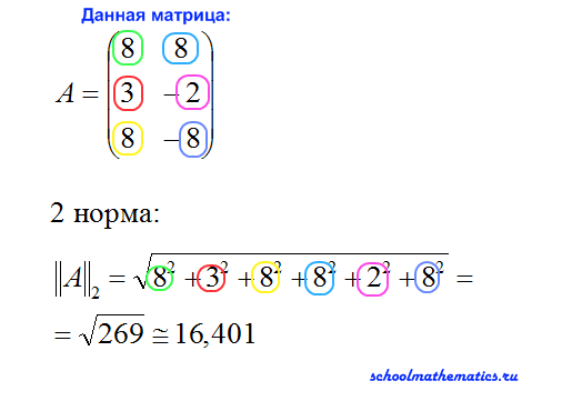
В
нашем случае, 2 норма матрицы получилась
равна квадратному корню из 269. На схеме,
я приближенно извлекла квадратный
корень из 269 и в результате получила
приблизительно около 16,401. Хотя более
правильно не извлекать корень.

3
норма матрицы представляет из себя
максимальное из чисел, полученных при
сложении всех элементов каждой строки,
взятых по модулю.

В

нашем примере: в первой строке стоят
элементы: 8, 8. Все элементы положительные.
Найдем их сумму: 8+8=16. В второй строке
стоят элементы: 3, -2. Один из элементов
отрицательный, поэтому при сложении
этих чисел, необходимо подставлять
модуль этого числа. Найдем их сумму:
3+2=5. В третьей строке стоят элементы 8,
и -8. Один из элементов отрицательный,
поэтому при сложении этих чисел,
необходимо подставлять модуль этого
числа. Найдем их сумму: 8+8=16. Максимальное
из этих трех чисел — это 16. Значит третья
норма матрицы равна 16.

Число
обусловленности квадратной матрицы A
определяется, как

k(A)
= ||A||·||A -1||

Число
обусловленности имеет следующее
значение: если машинная точность, с
которой совершаются все операции с
вещественными числами, равна ε, то при
решении системы линейных уравнений Ax
= b результат будет получен с относительной
погрешностью порядка ε·k(A). Хотя число
обусловленности матрицы зависит от
выбора нормы, если матрица хорошо
обусловлена, то её число обусловленности
будет мало при любом выборе нормы, а
если она плохо обусловлена, то её число
обусловленности будет велико при любом
выборе нормы. Таким образом, обычно
норму выбирают исходя из соображений
удобства. На практике наиболее широко
используют 1-норму, 2-норму и ∞-норму,
задающиеся формулами:

В
Matlab
используется следующие функции поиска
нормы:

Пусть
А —матрица. Тогда n=norm(A) эквивалентно
п=погп(А,2) и возвращает вторую норму, т.
е. самое большое сингулярное число А.
Функция n=norm(A, 1) возвращает первую норму,
т. е. самую большую из сумм абсолютных
значений элементов матрицы по столбцам.
Норма неопределенности n=norm(A, inf) возвращает
самую большую из сумм абсолютных значений
элементов матрицы по рядам. Норма
Фробениуса
(Frobenius) norm(A, ‘fro’) = sqrt(sum(diag(A’A))).

Пример:

»
A=[2,3,1;1,9,4;2,6,7]

A
=

2
3 1

1
9 4

2
6 7

»
norm(A,1)

ans
=

18

Числа
обусловленности матрицы определяют
чувствительность решения системы
линейных уравнений к погрешностям
исходных данных. Следующие функции
позволяют найти числа обусловленности
матриц.

cond(X)
— возвращает число обусловленности,
основанное на второй норме, то есть
отношение самого большого сингулярного
числа X к самому малому. Значение cond(X),
близкое к 1, указывает на хорошо
обусловленную матрицу;

с
= cond(X,p) — возвращает число обусловленности
матрицы, основанное на р-норме:
norm(X,p)*norm(inv(X),p), где р определяет способ
расчета:

р=1
— число обусловленности матрицы,
основанное на первой норме;

р=2
— число обусловленности матрицы,
основанное на второй норме;

p=
‘fro’ — число обусловленности матрицы,
основанное на норме Фробе-ниуса
(Frobenius);

р=’inf’
— число обусловленности матрицы,
основанное на норме неопределенности.

с
= cond(X) — возвращает число обусловленности
матрицы, основанное на второй норме.

Пример:

»
d=cond(hilb(4))

d
=

1.5514е+004

condeig(A)
— возвращает вектор чисел обусловленности
для собственных значений А. Эти числа
обусловленности — обратные величины
косинусов углов между левыми и правыми
собственными векторами;

[V.D.s]
= condeig(A) — эквивалентно
[V,D] = eig(A): s = condeig(A);.

Большие
числа обусловленности означают, что
матрица А близка к матрице с кратными
собственными значениями.

Пример:

»
d=condeig(rand(4))

d
=

1.0766

1.2298

1.5862

1.7540

rcond(A)
— возвращает обратную величину
обусловленности матрицы А по первой
норме, используя оценивающий обусловленность
метод LAPACK. Если А — хорошо обусловленная
матрица, то rcond(A) около 1.00, если плохо
обусловленная, то около 0.00. По сравнению
с cond функция rcond реализует более
эффективный в плане затрат машинного
времени, но менее достоверный метод
оценки обусловленности матрицы.

Пример:

»
s=rcond(hilb(4))

s
=

4.6461е-005

Соседние файлы в предмете [НЕСОРТИРОВАННОЕ]

• #
• #
• #
• #
• #
• #
• #
• #
• #
• #
• #

Линейная алгебра для исследователей данных

«Наша [Ирвинга Капланского и Пола Халмоша] общая философия в отношении линейной алгебры такова: мы думаем в безбазисных терминах, пишем в безбазисных терминах, но когда доходит до серьезного дела, мы запираемся в офисе и вовсю считаем с помощью матриц».

Ирвинг Капланский

Для многих начинающих исследователей данных линейная алгебра становится камнем преткновения на пути к достижению мастерства в выбранной ими профессии.

В этой статье я попытался собрать основы линейной алгебры, необходимые в повседневной работе специалистам по машинному обучению и анализу данных.

Произведения векторов 

Для двух векторов x, y ∈ ℝⁿ их скалярным или внутренним произведением xᵀy

называется следующее вещественное число:

Как можно видеть, скалярное произведение является особым частным случаем произведения матриц. Также заметим, что всегда справедливо тождество

.

Для двух векторов x ∈ ℝᵐ, y ∈ ℝⁿ (не обязательно одной размерности) также можно определить внешнее произведение xyᵀ ∈ ℝᵐˣⁿ. Это матрица, значения элементов которой определяются следующим образом: (xyᵀ)ᵢⱼ = xᵢyⱼ, то есть

След 

Следом квадратной матрицы A ∈ ℝⁿˣⁿ, обозначаемым tr(A) (или просто trA), называют сумму элементов на ее главной диагонали: 

След обладает следующими свойствами:

• Для любой матрицы A ∈ ℝⁿˣⁿ: trA = trAᵀ.

• Для любых матриц A,B ∈ ℝⁿˣⁿ: tr(A + B) = trA + trB.

• Для любой матрицы A ∈ ℝⁿˣⁿ и любого числа t ∈ ℝ: tr(tA) = t trA.

• Для любых матриц A,B, таких, что их произведение AB является квадратной матрицей: trAB = trBA.

• Для любых матриц A,B,C, таких, что их произведение ABC является квадратной матрицей: trABC = trBCA = trCAB (и так далее — данное свойство справедливо для любого числа матриц).

Нормы

Норму ∥x∥ вектора x можно неформально определить как меру «длины» вектора. Например, часто используется евклидова норма, или норма l₂:

Заметим, что ‖x‖₂²=xᵀx.

Более формальное определение таково: нормой называется любая функция f : ℝn → ℝ, удовлетворяющая четырем условиям:

1. Для всех векторов x ∈ ℝⁿ: f(x) ≥ 0 (неотрицательность).

2. f(x) = 0 тогда и только тогда, когда x = 0 (положительная определенность).

3. Для любых вектора x ∈ ℝⁿ и числа t ∈ ℝ: f(tx) = |t|f(x) (однородность).

4. Для любых векторов x, y ∈ ℝⁿ: f(x + y) ≤ f(x) + f(y) (неравенство треугольника)

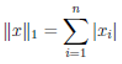
Другими примерами норм являются норма l₁

и норма l∞

Все три представленные выше нормы являются примерами норм семейства lp, параметризуемых вещественным числом p ≥ 1 и определяемых как

Нормы также могут быть определены для матриц, например норма Фробениуса:

Линейная независимость и ранг 

Множество векторов {x₁, x₂, …, xₙ} ⊂ ℝₘ называют линейно независимым, если никакой из этих векторов не может быть представлен в виде линейной комбинации других векторов этого множества. Если же такое представление какого-либо из векторов множества возможно, эти векторы называют линейно зависимыми. То есть, если выполняется равенство

для некоторых скалярных значений α₁,…, αₙ-₁ ∈ ℝ, то мы говорим, что векторы x₁, …, xₙ линейно зависимы; в противном случае они линейно независимы. Например, векторы

линейно зависимы, так как x₃ = −2xₙ + x₂.

Столбцовым рангом матрицы A ∈ ℝᵐˣⁿ называют число элементов в максимальном подмножестве ее столбцов, являющемся линейно независимым. Упрощая, говорят, что столбцовый ранг — это число линейно независимых столбцов A. Аналогично строчным рангом матрицы является число ее строк, составляющих максимальное линейно независимое множество.

Оказывается (здесь мы не будем это доказывать), что для любой матрицы A ∈ ℝᵐˣⁿ столбцовый ранг равен строчному, поэтому оба этих числа называют просто рангом A и обозначают rank(A) или rk(A); встречаются также обозначения rang(A), rg(A) и просто r(A). Вот некоторые основные свойства ранга:

• Для любой матрицы A ∈ ℝᵐˣⁿ: rank(A) ≤ min(m,n). Если rank(A) = min(m,n), то A называют матрицей полного ранга.

• Для любой матрицы A ∈ ℝᵐˣⁿ: rank(A) = rank(Aᵀ).

• Для любых матриц A ∈ ℝᵐˣⁿ, B ∈ ℝn×p: rank(AB) ≤ min(rank(A),rank(B)).

• Для любых матриц A,B ∈ ℝᵐˣⁿ: rank(A + B) ≤ rank(A) + rank(B).

Ортогональные матрицы 

Два вектора x, y ∈ ℝⁿ называются ортогональными, если xᵀy = 0. Вектор x ∈ ℝⁿ называется нормированным, если ||x||₂ = 1. Квадратная м

атрица U ∈ ℝⁿˣⁿ называется ортогональной, если все ее столбцы ортогональны друг другу и нормированы (в этом случае столбцы называют ортонормированными). Заметим, что понятие ортогональности имеет разный смысл для векторов и матриц.

Непосредственно из определений ортогональности и нормированности следует, что

Другими словами, результатом транспонирования ортогональной матрицы является матрица, обратная исходной. Заметим, что если U не является квадратной матрицей (U ∈ ℝᵐˣⁿ, n < m), но ее столбцы являются ортонормированными, то UᵀU = I, но UUᵀ ≠ I. Поэтому, говоря об ортогональных матрицах, мы будем по умолчанию подразумевать квадратные матрицы.

Еще одно удобное свойство ортогональных матриц состоит в том, что умножение вектора на ортогональную матрицу не меняет его евклидову норму, то есть

для любых вектора x ∈ ℝⁿ и ортогональной матрицы U ∈ ℝⁿˣⁿ.

Область значений и нуль-пространство матрицы

Линейной оболочкой множества векторов {x₁, x₂, …, xₙ} является множество всех векторов, которые могут быть представлены в виде линейной комбинации векторов {x₁, …, xₙ}, то есть

Областью значений R(A) (или пространством столбцов) матрицы A ∈ ℝᵐˣⁿ называется линейная оболочка ее столбцов. Другими словами,

 Нуль-пространством, или ядром матрицы A ∈ ℝᵐˣⁿ (обозначаемым N(A) или ker A), называют множество всех векторов, которые при умножении на A обращаются в нуль, то есть

Квадратичные формы и положительно полуопределенные матрицы 

Для квадратной матрицы A ∈ ℝⁿˣⁿ и вектора x ∈ ℝⁿ квадратичной формой называется скалярное значение xᵀ Ax. Распишем это выражение подробно:

Заметим, что

• Симметричная матрица A ∈ 𝕊ⁿ называется положительно определенной, если для всех ненулевых векторов x ∈ ℝⁿ справедливо неравенство xᵀAx > 0. Обычно это обозначается как

  

  (или просто A > 0), а множество всех положительно определенных матриц часто обозначают

  

  .

• Симметричная матрица A ∈ 𝕊ⁿ называется положительно полуопределенной, если для всех векторов справедливо неравенство xᵀ Ax ≥ 0. Это записывается как

  

  (или просто A ≥ 0), а множество всех положительно полуопределенных матриц часто обозначают

  

  .

• Аналогично симметричная матрица A ∈ 𝕊ⁿ называется отрицательно определенной

  

• , если для всех ненулевых векторов x ∈ ℝⁿ справедливо неравенство xᵀAx < 0.

• Далее, симметричная матрица A ∈ 𝕊ⁿ называется отрицательно полуопределенной (

  

  ), если для всех ненулевых векторов x ∈ ℝⁿ справедливо неравенство xᵀAx ≤ 0.

• Наконец, симметричная матрица A ∈ 𝕊ⁿ называется неопределенной, если она не является ни положительно полуопределенной, ни отрицательно полуопределенной, то есть если существуют векторы x₁, x₂ ∈ ℝⁿ такие, что

  

  и

  

  .

Собственные значения и собственные векторы 

Для квадратной матрицы A ∈ ℝⁿˣⁿ комплексное значение λ ∈ ℂ и вектор x ∈ ℂⁿ будут соответственно являться собственным значением и собственным вектором, если выполняется равенство

На интуитивном уровне это определение означает, что при умножении на матрицу A вектор x сохраняет направление, но масштабируется с коэффициентом λ. Заметим, что для любого собственного вектора x ∈ ℂⁿ и скалярного значения с ∈ ℂ справедливо равенство A(cx) = cAx = cλx = λ(cx). Таким образом, cx тоже является собственным вектором. Поэтому, говоря о собственном векторе, соответствующем собственному значению λ, мы обычно имеем в виду нормализованный вектор с длиной 1 (при таком определении все равно сохраняется некоторая неоднозначность, так как собственными векторами будут как x, так и –x, но тут уж ничего не поделаешь).

---

Перевод статьи был подготовлен в преддверии старта курса «Математика для Data Science». Также приглашаем всех желающих посетить бесплатный демоурок, в рамках которого рассмотрим понятие линейного пространства на примерах, поговорим о линейных отображениях, их роли в анализе данных и порешаем задачи.

• ЗАПИСАТЬСЯ НА ДЕМОУРОК

In mathematics, a norm is a function from a real or complex vector space to the non-negative real numbers that behaves in certain ways like the distance from the origin: it commutes with scaling, obeys a form of the triangle inequality, and is zero only at the origin. In particular, the Euclidean distance in a Euclidean space is defined by a norm on the associated Euclidean vector space, called the Euclidean norm, the 2-norm, or, sometimes, the magnitude of the vector. This norm can be defined as the square root of the inner product of a vector with itself.

A seminorm satisfies the first two properties of a norm, but may be zero for vectors other than the origin.^[1] A vector space with a specified norm is called a normed vector space. In a similar manner, a vector space with a seminorm is called a seminormed vector space.

The term pseudonorm has been used for several related meanings. It may be a synonym of «seminorm».^[1]
A pseudonorm may satisfy the same axioms as a norm, with the equality replaced by an inequality «» in the homogeneity axiom.^[2]
It can also refer to a norm that can take infinite values,^[3] or to certain functions parametrised by a directed set.^[4]

Definition[edit]

Given a vector space over a subfield of the complex numbers a norm on is a real-valued function with the following properties, where denotes the usual absolute value of a scalar :^[5]

1. Subadditivity/Triangle inequality: for all
2. Absolute homogeneity: for all and all scalars
3. Positive definiteness/positiveness^[6]/Point-separating: for all if then

A seminorm on is a function that has properties (1.) and (2.)^[7] so that in particular, every norm is also a seminorm (and thus also a sublinear functional). However, there exist seminorms that are not norms. Properties (1.) and (2.) imply that if is a norm (or more generally, a seminorm) then and that also has the following property:

2. Non-negativity:^[6] for all

Some authors include non-negativity as part of the definition of «norm», although this is not necessary.
Although this article defined «positive» to be a synonym of «positive definite», some authors instead define «positive» to be a synonym of «non-negative»;^[8] these definitions are not equivalent.

Equivalent norms[edit]

Suppose that and are two norms (or seminorms) on a vector space Then and are called equivalent, if there exist two positive real constants and with such that for every vector

The relation « is equivalent to » is reflexive, symmetric ( implies ), and transitive and thus defines an equivalence relation on the set of all norms on
The norms and are equivalent if and only if they induce the same topology on ^[9] Any two norms on a finite-dimensional space are equivalent but this does not extend to infinite-dimensional spaces.^[9]

Notation[edit]

If a norm is given on a vector space then the norm of a vector is usually denoted by enclosing it within double vertical lines: Such notation is also sometimes used if is only a seminorm. For the length of a vector in Euclidean space (which is an example of a norm, as explained below), the notation with single vertical lines is also widespread.

Examples[edit]

Every (real or complex) vector space admits a norm: If is a Hamel basis for a vector space then the real-valued map that sends (where all but finitely many of the scalars are ) to is a norm on ^[10] There are also a large number of norms that exhibit additional properties that make them useful for specific problems.

Absolute-value norm[edit]

The absolute value

is a norm on the one-dimensional vector spaces formed by the real or complex numbers.

Any norm on a one-dimensional vector space is equivalent (up to scaling) to the absolute value norm, meaning that there is a norm-preserving isomorphism of vector spaces where is either or and norm-preserving means that
This isomorphism is given by sending to a vector of norm which exists since such a vector is obtained by multiplying any non-zero vector by the inverse of its norm.

Euclidean norm[edit]

On the -dimensional Euclidean space the intuitive notion of length of the vector is captured by the formula^[11]

This is the Euclidean norm, which gives the ordinary distance from the origin to the point X—a consequence of the Pythagorean theorem.
This operation may also be referred to as «SRSS», which is an acronym for the square root of the sum of squares.^[12]

The Euclidean norm is by far the most commonly used norm on ^[11] but there are other norms on this vector space as will be shown below.
However, all these norms are equivalent in the sense that they all define the same topology.

The inner product of two vectors of a Euclidean vector space is the dot product of their coordinate vectors over an orthonormal basis.
Hence, the Euclidean norm can be written in a coordinate-free way as

The Euclidean norm is also called the norm,^[13] norm, 2-norm, or square norm; see space.
It defines a distance function called the Euclidean length, distance, or distance.

The set of vectors in whose Euclidean norm is a given positive constant forms an -sphere.

Euclidean norm of complex numbers[edit]

The Euclidean norm of a complex number is the absolute value (also called the modulus) of it, if the complex plane is identified with the Euclidean plane This identification of the complex number as a vector in the Euclidean plane, makes the quantity (as first suggested by Euler) the Euclidean norm associated with the complex number.

Quaternions and octonions[edit]

There are exactly four Euclidean Hurwitz algebras over the real numbers. These are the real numbers the complex numbers the quaternions and lastly the octonions where the dimensions of these spaces over the real numbers are respectively.
The canonical norms on and are their absolute value functions, as discussed previously.

The canonical norm on of quaternions is defined by

for every quaternion in This is the same as the Euclidean norm on considered as the vector space Similarly, the canonical norm on the octonions is just the Euclidean norm on

Finite-dimensional complex normed spaces[edit]

On an -dimensional complex space the most common norm is

In this case, the norm can be expressed as the square root of the inner product of the vector and itself:

where is represented as a column vector and denotes its conjugate transpose.

This formula is valid for any inner product space, including Euclidean and complex spaces. For complex spaces, the inner product is equivalent to the complex dot product. Hence the formula in this case can also be written using the following notation:

Taxicab norm or Manhattan norm[edit]

The name relates to the distance a taxi has to drive in a rectangular street grid (like that of the New York borough of Manhattan) to get from the origin to the point

The set of vectors whose 1-norm is a given constant forms the surface of a cross polytope of dimension equivalent to that of the norm minus 1.
The Taxicab norm is also called the norm. The distance derived from this norm is called the Manhattan distance or distance.

The 1-norm is simply the sum of the absolute values of the columns.

In contrast,

is not a norm because it may yield negative results.

p-norm[edit]

Let be a real number.
The -norm (also called -norm) of vector is^[11]

For we get the taxicab norm, for we get the Euclidean norm, and as approaches the -norm approaches the infinity norm or maximum norm:

The -norm is related to the generalized mean or power mean.

For the -norm is even induced by a canonical inner product meaning that for all vectors This inner product can be expressed in terms of the norm by using the polarization identity.
On this inner product is the Euclidean inner product defined by

while for the space associated with a measure space which consists of all square-integrable functions, this inner product is

This definition is still of some interest for but the resulting function does not define a norm,^[14] because it violates the triangle inequality.
What is true for this case of even in the measurable analog, is that the corresponding class is a vector space, and it is also true that the function

(without th root) defines a distance that makes into a complete metric topological vector space. These spaces are of great interest in functional analysis, probability theory and harmonic analysis.
However, aside from trivial cases, this topological vector space is not locally convex, and has no continuous non-zero linear forms. Thus the topological dual space contains only the zero functional.

The partial derivative of the -norm is given by

The derivative with respect to therefore, is

where denotes Hadamard product and is used for absolute value of each component of the vector.

For the special case of this becomes

or

Maximum norm (special case of: infinity norm, uniform norm, or supremum norm)[edit]

If is some vector such that then:

The set of vectors whose infinity norm is a given constant, forms the surface of a hypercube with edge length

Zero norm[edit]

In probability and functional analysis, the zero norm induces a complete metric topology for the space of measurable functions and for the F-space of sequences with F–norm ^[15]
Here we mean by F-norm some real-valued function on an F-space with distance such that The F-norm described above is not a norm in the usual sense because it lacks the required homogeneity property.

Hamming distance of a vector from zero[edit]

In metric geometry, the discrete metric takes the value one for distinct points and zero otherwise. When applied coordinate-wise to the elements of a vector space, the discrete distance defines the Hamming distance, which is important in coding and information theory.
In the field of real or complex numbers, the distance of the discrete metric from zero is not homogeneous in the non-zero point; indeed, the distance from zero remains one as its non-zero argument approaches zero.
However, the discrete distance of a number from zero does satisfy the other properties of a norm, namely the triangle inequality and positive definiteness.
When applied component-wise to vectors, the discrete distance from zero behaves like a non-homogeneous «norm», which counts the number of non-zero components in its vector argument; again, this non-homogeneous «norm» is discontinuous.

In signal processing and statistics, David Donoho referred to the zero «norm« with quotation marks.
Following Donoho’s notation, the zero «norm» of is simply the number of non-zero coordinates of or the Hamming distance of the vector from zero.
When this «norm» is localized to a bounded set, it is the limit of -norms as approaches 0.
Of course, the zero «norm» is not truly a norm, because it is not positive homogeneous.
Indeed, it is not even an F-norm in the sense described above, since it is discontinuous, jointly and severally, with respect to the scalar argument in scalar–vector multiplication and with respect to its vector argument.
Abusing terminology, some engineers^[who?] omit Donoho’s quotation marks and inappropriately call the number-of-non-zeros function the norm, echoing the notation for the Lebesgue space of measurable functions.

Infinite dimensions[edit]

The generalization of the above norms to an infinite number of components leads to and spaces, with norms

for complex-valued sequences and functions on respectively, which can be further generalized (see Haar measure).

Any inner product induces in a natural way the norm

Other examples of infinite-dimensional normed vector spaces can be found in the Banach space article.

Composite norms[edit]

Other norms on can be constructed by combining the above; for example

is a norm on

For any norm and any injective linear transformation we can define a new norm of equal to

In 2D, with a rotation by 45° and a suitable scaling, this changes the taxicab norm into the maximum norm. Each applied to the taxicab norm, up to inversion and interchanging of axes, gives a different unit ball: a parallelogram of a particular shape, size, and orientation.

In 3D, this is similar but different for the 1-norm (octahedrons) and the maximum norm (prisms with parallelogram base).

There are examples of norms that are not defined by «entrywise» formulas. For instance, the Minkowski functional of a centrally-symmetric convex body in (centered at zero) defines a norm on (see § Classification of seminorms: absolutely convex absorbing sets below).

All the above formulas also yield norms on without modification.

There are also norms on spaces of matrices (with real or complex entries), the so-called matrix norms.

In abstract algebra[edit]

Let be a finite extension of a field of inseparable degree and let have algebraic closure If the distinct embeddings of are then the Galois-theoretic norm of an element is the value As that function is homogeneous of degree , the Galois-theoretic norm is not a norm in the sense of this article. However, the -th root of the norm (assuming that concept makes sense) is a norm.^[16]

Composition algebras[edit]

The concept of norm in composition algebras does not share the usual properties of a norm as it may be negative or zero for A composition algebra consists of an algebra over a field an involution and a quadratic form called the «norm».

The characteristic feature of composition algebras is the homomorphism property of : for the product of two elements and of the composition algebra, its norm satisfies For and O the composition algebra norm is the square of the norm discussed above. In those cases the norm is a definite quadratic form. In other composition algebras the norm is an isotropic quadratic form.

Properties[edit]

For any norm on a vector space the reverse triangle inequality holds:

If is a continuous linear map between normed spaces, then the norm of and the norm of the transpose of are equal.^[17]

For the norms, we have Hölder’s inequality^[18]

A special case of this is the Cauchy–Schwarz inequality:^[18]

Every norm is a seminorm and thus satisfies all properties of the latter. In turn, every seminorm is a sublinear function and thus satisfies all properties of the latter. In particular, every norm is a convex function.

Equivalence[edit]

The concept of unit circle (the set of all vectors of norm 1) is different in different norms: for the 1-norm, the unit circle is a square, for the 2-norm (Euclidean norm), it is the well-known unit circle, while for the infinity norm, it is a different square. For any -norm, it is a superellipse with congruent axes (see the accompanying illustration). Due to the definition of the norm, the unit circle must be convex and centrally symmetric (therefore, for example, the unit ball may be a rectangle but cannot be a triangle, and for a -norm).

In terms of the vector space, the seminorm defines a topology on the space, and this is a Hausdorff topology precisely when the seminorm can distinguish between distinct vectors, which is again equivalent to the seminorm being a norm. The topology thus defined (by either a norm or a seminorm) can be understood either in terms of sequences or open sets. A sequence of vectors is said to converge in norm to if as Equivalently, the topology consists of all sets that can be represented as a union of open balls. If is a normed space then^[19]

Two norms and on a vector space are called equivalent if they induce the same topology,^[9] which happens if and only if there exist positive real numbers and such that for all

For instance, if on then^[20]

In particular,

That is,

If the vector space is a finite-dimensional real or complex one, all norms are equivalent. On the other hand, in the case of infinite-dimensional vector spaces, not all norms are equivalent.

Equivalent norms define the same notions of continuity and convergence and for many purposes do not need to be distinguished. To be more precise the uniform structure defined by equivalent norms on the vector space is uniformly isomorphic.

Classification of seminorms: absolutely convex absorbing sets[edit]

All seminorms on a vector space can be classified in terms of absolutely convex absorbing subsets of To each such subset corresponds a seminorm called the gauge of defined as

where is the infimum, with the property that

Conversely:

Any locally convex topological vector space has a local basis consisting of absolutely convex sets. A common method to construct such a basis is to use a family of seminorms that separates points: the collection of all finite intersections of sets turns the space into a locally convex topological vector space so that every p is continuous.

Such a method is used to design weak and weak* topologies.

norm case:

Suppose now that contains a single since is separating, is a norm, and is its open unit ball. Then is an absolutely convex bounded neighbourhood of 0, and is continuous.

The converse is due to Andrey Kolmogorov: any locally convex and locally bounded topological vector space is normable. Precisely:

If is an absolutely convex bounded neighbourhood of 0, the gauge (so that is a norm.

See also[edit]

• Asymmetric norm – Generalization of the concept of a norm
• F-seminorm – A topological vector space whose topology can be defined by a metric
• Gowers norm
• Kadec norm – All infinite-dimensional, separable Banach spaces are homeomorphic
• Least-squares spectral analysis – Periodicity computation method
• Mahalanobis distance – Statistical distance measure
• Magnitude (mathematics) – mathematical concept related to comparison and ordering
• Matrix norm – Norm on a vector space of matrices
• Minkowski distance – distance between vectors or points computed as the pth root of the sum of pth powers of coordinate differences
• Minkowski functional
• Operator norm – Measure of the «size» of linear operators
• Paranorm – A topological vector space whose topology can be defined by a metric
• Relation of norms and metrics – Mathematical space with a notion of distance
• Seminorm – nonnegative-real-valued function on a real or complex vector space that satisfies the triangle inequality and is absolutely homogenous
• Sublinear function

References[edit]

Bibliography[edit]

• Bourbaki, Nicolas (1987) [1981]. Topological Vector Spaces: Chapters 1–5. Éléments de mathématique. Translated by Eggleston, H.G.; Madan, S. Berlin New York: Springer-Verlag. ISBN 3-540-13627-4. OCLC 17499190.
• Khaleelulla, S. M. (1982). Counterexamples in Topological Vector Spaces. Lecture Notes in Mathematics. Vol. 936. Berlin, Heidelberg, New York: Springer-Verlag. ISBN 978-3-540-11565-6. OCLC 8588370.
• Kubrusly, Carlos S. (2011). The Elements of Operator Theory (Second ed.). Boston: Birkhäuser Basel. ISBN 978-0-8176-4998-2. OCLC 710154895.
• Narici, Lawrence; Beckenstein, Edward (2011). Topological Vector Spaces. Pure and applied mathematics (Second ed.). Boca Raton, FL: CRC Press. ISBN 978-1584888666. OCLC 144216834.
• Schaefer, Helmut H.; Wolff, Manfred P. (1999). Topological Vector Spaces. GTM. Vol. 8 (Second ed.). New York, NY: Springer New York Imprint Springer. ISBN 978-1-4612-7155-0. OCLC 840278135.
• Trèves, François (2006) [1967]. Topological Vector Spaces, Distributions and Kernels. Mineola, N.Y.: Dover Publications. ISBN 978-0-486-45352-1. OCLC 853623322.
• Wilansky, Albert (2013). Modern Methods in Topological Vector Spaces. Mineola, New York: Dover Publications, Inc. ISBN 978-0-486-49353-4. OCLC 849801114.

У этого термина существуют и другие значения, см. норма.

Норма — понятие, обобщающее абсолютную величину (модуль) числа, а также длину вектора на случай элементов (векторов) линейного пространства.

Норма в векторном линейном пространстве над полем вещественных или комплексных чисел есть функция , удовлетворяющая следующим условиям:

1. , причём только при ;
2. для всех (неравенство треугольника);
3. для каждого скаляра .

Норма обычно обозначается . Линейное пространство с нормой называется нормированным пространством.

Примеры норм в линейных пространствах

Топология пространства и норма

Норма задаёт на пространстве топологию, базой которой являются всевозможные открытые шары, то есть множества вида . Понятия сходимости, определённой на языке теоретико-множественной топологии в такой топологии и определённой на языке нормы, при этом совпадают.

Эквивалентность норм

Две нормы и на пространстве называются эквивалентными, если существует две положительные константы и такие, что для любого выполняется . Эквивалентные нормы задают на пространстве одинаковую топологию. В конечномерном пространстве все нормы эквивалентны.

Операторная норма

Норма оператора — число, которое определяется, как:

.

где — оператор, действующий из нормированного пространства в нормированное пространство .

• Свойства операторных норм:

1. , причём только при ;
2. ;
3. ;
4. .

Матричная норма

Нормой матрицы называется действительное число , удовлетворяющее первым трём из следующих условий:

1. , причём только при ;
2. ;
3. ;
4. .

Если выполняется также и четвёртое свойство, норма называется мультипликативной. Матричная норма, составленная как операторная, называется подчинённой по отношению к норме, использованной в пространствах векторов. Очевидно, что все подчинённые матричные нормы мультипликативны. Немультипликативные нормы для матриц являются простыми нормами, заданными в линейных пространствах матриц.

Виды матричных норм

1. m-норма:
2. l-норма:
3. Евклидова норма:
4. Сингулярная норма (подчинена евклидовой норме векторов):

ca:Norma (matemàtiques)
da:Norm (matematik)
he:נורמה (מתמטיקה)
nl:Norm (wiskunde)
pl:Norma (matematyka)
sv:Norm (matematik)
ur:امثولہ (ریاضی)

Норма алгебраического числа — теоретико-числовая функция, норма, определённая в конечном алгебраическом расширении поля. Норма алгебраического числа равна произведению всех корней минимального многочлена данного числа. Норма отображает кольцо целых элементов расширения поля в кольцо целых элементов поля. Часто в качестве поля берется поле рациональных чисел , а значит в качестве кольца его целых элементов берется кольцо целых чисел .

Свойства

• Норма — мультипликативная функция.
• Норма отображает обратимые элементы кольца в обратимые элементы кольца.
• Норма сохраняет отношение делимости элементов кольца, в частности, норма простого элемента кольца равна простому элементу кольца

Примеры

Норма в кольце гауссовых целых чисел

Поле — расширение поля рациональных чисел, кольцо его целых элементов — это кольцо гауссовых целых чисел чисел вида . Норма определяется как . Для данной нормы — простое число в тогда и только тогда, когда — простой элемент кольца . Таким образом, в 2 и все простые числа вида разложимы в , а простые вида — неразложимы, поэтому .

Множество обратимых элементов кольца состоит из 4-х элементов: , норма только этих элементов равна 1.

Норма в действительном квадратичной расширении кольца целых чисел

Если — натуральное число, свободное от квадратов, то — действительное квадратичное расширение кольца степени 2, его элементы имеют вид . Норма в определяется как . Множество обратимых элементов кольца состоит из бесконечного множества элементов — всех решений уравнения Пелля .

Применение

Норма применяется для решения диофантовых уравнений. Если уравнение имеет вид , где F — норма N некоторого кольца алгебраических чисел K, а — элемент кольца, определенный энкой , то для решения уравнения достаточно найти хотя бы одно решение уравнения и все обратимые элементы кольца . Так могут быть решены обобщенные уравнения Пелля вида .

Норма может применятся для исследования простых элементов колец алгебраических чисел и простых элементов кольца .

Литература

• Боревич З.И. Шафаревич И.Р. Теория чисел. — ФизМатЛит, 1985.
• Постников М.М. Высшая геометрия. — ФизМатЛит, 1982.