Как найти объемное смещение - Исправление недочетов и поиск решений вместе с Examum.ru

Смещенный объем

Смещенный объем – прибавленный или
удаленный в процессе деформации объем
в направлении одной из осей. Если
рассматривать деформацию по высоте,
смещенный объем – произведение начальной
площади поперечного сечения на абсолютное
обжатие.

Для более точных расчетов необходимо
интегрировать по всему

диапазону изменений высоты:

— истинный смещенный объем

V_dh
+ V_db
+ V_dL
= V
(ln

+ ln

+ ln

)
= 0, т.е. сумма истинных смещенных
объемов по трем главным осям равна нулю.

Если по некоторой оси происходит
уменьшение размеров тела, то истинный
смещенный объем меньше нуля, если
увеличение – больше нуля. Смещенный
объем может быть равен, больше или меньше
реального объема тела. Поскольку по
высоте происходит уменьшение размера,
т.е. h₁<h₀, то

будет
отрицательным. Смещенный объем по
величине равен истинному объему тела,
если

,
т.е.

,
или если

,
т.е.

.
Таким образом, истинный смещенный объем
будет больше объема тела, когда h<0.368
или

>2.718
(т.е.

>0.632
или

<1.718).

Общий случай деформации

общем случае деформация нелинейная, а
значит, кроме растяжения или сжатия в
металле имеется и угловая деформация,
т.е. кручение. А значит, в общем виде
деформированное состояние в точке
определяется не только линейными
деформациями, но и деформациями сдвига.

Рассмотрим деформацию элемента
прямоугольной формы, расположенного в
окрестностях произвольной точки (см.
рисунок). Растяжение элемента вдоль
трех осей определяется тремя линейными
деформациями

где u – проекция
перемещения точки на ось x,
v – на ось y, w – на ось z.

Изгиб элемента определяется шестью
деформациями сдвига

:

Относительная деформация сдвига
определяется углом между направлениями
ребер в исходном состоянии и после
деформации (при линейной деформации
углы и деформации сдвига равны нулю),
т.е.

.

Таким образом,
напряженное состояние в точке определяется
тензором деформаций:

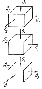
каждой точке тела существуют оси
деформации, которые называют главными
осями деформации. Эти оси обладают
тем свойством, что волокна в теле, им
перпендикулярные, испытывают только
линейные деформации (укорачиваются или
удлиняются), но не поворачиваются, т.е.
сдвиги в главных осях деформации равны
нулю. Деформации вдоль главных осей
называются главными деформациями и
обозначаются

.
Тензор деформаций в главных осях имеет
вид:

Существуют 3 схемы главных деформаций:
две объемные (растяжение-растяжение-сжатие
и растяжение-сжатие-сжатие) и одна
плоская (растяжение-сжатие, по третьей
оси деформации нет). Из закона постоянства
объема следует, что все главные деформации
не могу быть одного знака, т.е. растяжение
или сжатие не может быть по всем осям
осям одновременно.

Скорость деформации

Скорость деформации – изменение
степени деформации в единицу времени.
Совокупность всех скоростей деформации
описывается тензором скоростей
деформации:

,
где

Из формул
видно, что размерность скорости деформации
– c^-1.

Скорость
деформирования – скорость хода
инструмента. Единица измерения – м/с.
Скорость деформации зависит от скорости
деформирования и размера тела в
направлении деформации.

,
где V_h
– скорость деформирования.

Даже если
скорость движения инструмента постоянна,
скорость деформации изменяется из-за
изменения размеров заготовки. Средняя
скорость деформации за время обработки:

Скорости
деформации, соответствующие главным
направлениям, называются главными
скоростями деформации.

Соседние файлы в предмете [НЕСОРТИРОВАННОЕ]

Источник

Теоретическое объемное смещение с учетом площади поршня и длины хода Решение

ШАГ 0: Сводка предварительного расчета

ШАГ 1. Преобразование входов в базовый блок

Количество поршней: 5 —> Конверсия не требуется
Площадь поршня: 0.02 Квадратный метр —> 0.02 Квадратный метр Конверсия не требуется
Длина хода поршневого насоса: 0.2 метр —> 0.2 метр Конверсия не требуется

ШАГ 2: Оцените формулу

ШАГ 3: Преобразуйте результат в единицу вывода

0.02 Кубический метр на оборот —> Конверсия не требуется

19 Поршневые насосы Калькуляторы

Теоретическое объемное смещение с учетом площади поршня и длины хода формула

Теоретическое объемное смещение = Количество поршней*Площадь поршня*Длина хода поршневого насоса

V_D = n*A_p*SL

Каковы применения поршневых насосов?

Поршневые насосы используются в водяной и масляной гидравлике, промышленном технологическом оборудовании, очистке под высоким давлением и перекачивании жидкостей.

Источник

Просто щелкните объект решения правой кнопкой мыши и выберите «Вставить — Деформация — Всего». Это позволит рассчитать деформацию и смещение для всех тел в системе. Вы также можете рассчитать отклонения по определенным осям и для определенных тел или элементов.

Как найти узловое смещение в ANSYS Workbench?

Вы должны выбрать инструмент выбора узла и выбрать узлы из созданной структуры сетки.

Выберите необходимые узлы для именованного выбора.
Нажмите «Узловое смещение».
Выберите необходимый именованный выбор для «Узлового смещения».
Задайте величины узлового смещения.

Что такое поддержка смещения в ANSYS?

Опоры смещения используются для применения вынужденных перемещений и свободных перемещений в соответствующем направлении (X, Y и Z) в соответствии с условиями поддержки. Смещение такое же, как у фиксированной опоры, когда все поступательные движения равны нулю.

Что такое дистанционное смещение в ANSYS Workbench?

С помощью граничного условия Удаленное смещение можно указать управляемое смещение грани или объема с удаленной точкой.

Что такое поддержка только сжатия в Ansys Workbench?

Опора только на сжатие создает контакт без трения с жесткой поверхностью. Это как засунуть булавку в дырку. Нагрузка на подшипник создает силу в узлах, где максимальная сила находится под углом 0 градусов, а нулевая сила находится под углом 90 градусов с каждой стороны, а распределение силы является синусоидальным.

Что такое датчик деформации Ansys?

Ansys Mechanical Workbench поддерживает датчики деформации, которые на твердых телах могут измерять UX, UY, UZ и USUM геометрии или удаленных точек. Они не измеряют вращение. В этой статье показано, как использовать команды APDL для ссылки на существующую удаленную точку и измерения смещения и поворота в этой точке.

Как рассчитать узловое смещение?

Вкратце процедура в классе такова:

Удалите строки и столбцы, соответствующие степеням свободы с заданным смещением/поворотом (bc задано смещение=0) из матрицы жесткости.
Удалите строки, соответствующие заданному вектору нагрузки степеней свободы.
Решите редуцированную систему уравнений, чтобы получить неизвестные перемещения.

Что такое узловое смещение?

Узлы будут иметь узловые (векторные) смещения или степени свободы, которые могут включать перемещения, повороты и, для специальных приложений, производные перемещений более высокого порядка. Когда узлы смещаются, они будут тянуть элементы определенным образом, продиктованным формулировкой элемента.

Грубый. Подобно настройке без трения, эта настройка моделирует совершенно грубый фрикционный контакт, в котором отсутствует скольжение. Он применяется только к областям граней (для 3D-тел) или ребер (для 2D-пластин). По умолчанию автоматическое закрытие гэпов не выполняется.

Как добавить фиксированную поддержку в Ansys?

Чтобы добавить фиксированную поддержку в ANSYS® Mechanical, щелкните грани, вершины или ребра, которым вы хотите назначить фиксированную поддержку, затем нажмите «Применить к разделу геометрии», как показано красной стрелкой выше. Назначается фиксированная поддержка.

Что такое поддержка без трения в Ansys?

Это тип поддержки, используемый для ограниченных степеней свободы в нормальных направлениях. Это опорное или граничное условие используется для предотвращения перемещения или деформации одной или нескольких плоских или изогнутых граней в нормальном направлении.

Как сделать удаленное смещение в Ansys?

Нажмите «Удаленное смещение». Чтобы определить удаленное смещение, щелкните правой кнопкой мыши анализ, как показано выше. Затем наведите курсор на «Вставить» и нажмите «Удаленное смещение», чтобы определить его в ANSYS® Mechanical. Выберите геометрические особенности для «Удаленного смещения».

В чем разница между смещением и удаленным смещением в Ansys?

Лучшие ответы. См. документацию по смещению и удаленному смещению — вкратце смещение применяется к узлам на этом ребре (выходит как команда D в файле ds.dat), при этом удаленное смещение не обязательно должно быть на ребре, оно может быть точкой вне модели.

Что дает дистанционное перемещение?

Дистанционное смещение позволяет передать в систему эффекты известного смещения любого удаленного элемента конструкции, связанного с конструкцией жесткой связью.

Источник

Плотность тока проводимости, смещения, насыщения: определение и формулы

В данной статье мы рассмотрим плотность тока и формулы для нахождения различных видов плотности тока: проводимости, смещения, насыщения.

Плотность тока – это векторная физическая величина, характеризующая насколько плотно друг к другу располагаются электрические заряды.

Плотность тока проводимости

Ток проводимости – это упорядоченное движение электрических зарядов, то есть обыкновенный электрический ток, который возникает в проводнике. В большинстве случаев, когда речь заходит о токе, имеют ввиду именно ток проводимости.

В данном случае плотность тока – это векторная характеристика тока равная отношению силы тока I в проводнике к площади S поперечного сечения проводника (перпендикулярному по отношению к направлению тока). Эта величина показывает насколько плотно заряды располагаются на всей площади поперечного сечения проводника. Она обозначается латинской буквой j. Модуль плотности электрического тока пропорционален электрическому заряду, который протекает за определенное время через определенную площадь сечения, расположенную перпендикулярно по отношению к его направлению.

Если рассмотреть идеализированной проводник, в котором электрический ток равномерно распределен по всему сечению проводника, то модуль плотности тока проводимости можно вычислить по следующей формуле:

j – Плотность тока [A/м 2 ]

S – Площадь поперечного сечения проводника [м 2 ]

Исходя из этого мы можем представить силу тока I как поток вектора плотности тока j, проходящий через поперечное сечение проводникаS. То есть для вычисления силы тока, текущей через определенное поперечное сечение нужно проинтегрировать (сложить) произведения плотности тока в каждой точке проводника j_n на площадь поверхности этой точки dS:

j_n — составляющая вектора плотности тока в направлении течения тока (по оси OX) [A/м 2 ]

dS — элемент поверхности площади [м 2 ]

Исходя из предположения, что все заряженные частицы двигаются с одинаковым вектором скорости v, имеют одинаковые по величине заряды e и их концентрация n в каждой точке одинаковая, получаем, что плотность тока проводимости j равна:

j – плотность тока [А/м 2 ]

n – концентрация зарядов [м -3 ]

e – величина заряда [Кл]

v – скорость, с которой движутся частицы [м/с]

Плотность тока смещения

В классической электродинамике существует понятие тока смещения, который пропорционально равен быстроте изменения индукции электрического поля. Он не связан с перемещением каких-либо частиц поэтому, по сути, не является электрическим током. Несмотря на то, что природа этих токов разная, единица измерения плотности у них одинаковая — A/м 2 .

Ток смещения – это поток вектора быстроты изменения электрического поля ∂E/∂t через S — некоторую поверхность. Формула тока смещения выглядит так:

ε₀ – электрическая постоянная, равная 8,85·10 -12 Кл 2 /(H·м 2 )

∂E/∂t — скорость изменения электрического поля [Н/(Кл·с)]

ds – площадь поверхности [м 2 ]

Плотность тока смещения определяется по следующей формуле:

ε₀ – электрическая постоянная, равная 8,85·10 -12 Кл 2 /(H·м 2 )

∂E/∂t — скорость изменения электрического поля [Н/(Кл·с)]

∂D/∂t — скорость изменения вектора эл. индукции [Кл/м 2 ·с)]

Плотность тока насыщения

В физической электронике используют понятие плотности тока насыщения. Эта величина характеризует эмиссионную способность металла, из которого сделан катод, и зависит от его вида и температуры.

Плотность тока насыщения выражается формулой, которая была выведена на основе квантовой статистики Ричардсоном и Дешманом:

j – плотность тока насыщения[А/м 2 ]

R — среднее значение коэффициента отражения электронов от потенциального барьера

A — термоэлектрическая постоянная со значением 120,4 А/(K 2 ·см 2 )

T— температура [К]

qφ — значение работы выхода из катода электронов [эВ], q – электронный заряд [Кл]

k — постоянная Больцмана, которая равна 1,38·10 -23 Дж/К

Понравилась статья, расскажите о ней друзьям:

Ток смещения

Вы будете перенаправлены на Автор24

Физическое содержание тока смещения

Мы знаем, что постоянный ток в цепи с конденсатором не течет, переменный — протекает. Сила квазистационарного тока во всех элементах цепи, если они соединяются последовательно, одинакова. В конденсаторе, обкладки которого разделяет диэлектрик, ток проводимости, вызванный перемещением электронов, идти не может. Значит, если ток переменный (присутствует переменное электрическое поле), происходит некоторый процесс, который замыкает ток проводимости без переноса заряда между обкладками конденсатора. Этот процесс называют током смещения.

Любое переменное магнитное поле порождает вихревое электрическое поле. Исследуя разные электромагнитные процессы, Максвелл сделал вывод о том, что существует обратное явление: изменение электрического поля вызывает появление вихревого магнитного поля. Это одно из основных утверждений в теории Максвелла.

Так как магнитное поле — обязательный признак любого тока, Максвелл назвал переменное электрическое поле током смещения. Ток смещения следует отличать от тока проводимости, который вызван движением заряженных частиц (электронов и ионов). Токи смещения появляются только в том случае, если электрическое смещение ($overrightarrow$) переменно. Объемная плотность тока смещения определяется как:

Именно вследствие этого физическое содержание предположения Максвелла о токах смещения сводится к утверждению о том, что переменные электрические поля — источники переменных магнитных полей.

Следует заметить, что плотность тока смещения определена производной вектора $overrightarrow$, а не самим вектором.

Готовые работы на аналогичную тему

Ток смещения в диэлектрике

По определению вектора электрической индукции ($overrightarrow$):

где $<varepsilon >_0$ — электрическая постоянная, $overrightarrow$ — вектор напряженность, $overrightarrow

$ — вектор поляризации. Следовательно, ток смещения можно записать как:

где величина $frac<partial overrightarrow

><partial t>$ — плотность тока поляризации. Токи поляризации — токи, которые вызваны движением связанных зарядов, которые принципиально не отличаются от свободных зарядов. Поэтому нет ни чего странного, что токи поляризации порождают магнитное поле. Принципиальная новизна содержится в утверждении, что вторая часть тока смещения ($<varepsilon >_0frac<partial overrightarrow><partial t>$), не связанная с движением зарядов, также порождает магнитное поле. Получается, что в вакууме, любое изменение электрического поля по времени вызывает магнитное поле.

Однако, надо заметить, что сам термин «ток смещения» для диэлектриков имеет какое-то обоснование, так как в них действительно происходит смещение зарядов в атомах и молекулах. Но этот термин применяется и к вакууму, где зарядов нет, значит, нет их смещения.

Полный ток

В том случае, если в проводнике течет переменный ток, то внутри него имеется переменное электрическое поле. Значит, в проводнике существует ток проводимости ($j$) и ток смещения. Магнитное поле проводника определено суммой вышеназванных токов, то есть полным током ($overrightarrow$):

В зависимости от электропроводности вещества, частоты переменного тока, слагаемые в выражении (4), играют разную роль. В веществах с хорошей проводимостью (например, металлах) и при низких частотах переменного тока плотность тока смещения невелика, тогда как ток проводимости существенен. В таком случае, током смещения пренебрегают, в сравнении с током проводимости. В веществах с высоким сопротивлением (изоляторах) и при больших частотах тока ведущую роль играет ток смещения.

Оба слагаемых в выражении (4) могут иметь одинаковые знаки и противоположные. Следовательно, полный ток может быть и больше и меньше тока проводимости, может даже быть равен нулю.

Значит, в общем случае переменных токов магнитное поле определяется полным током. Если контур разомкнут, то на концах проводника обрывается только ток проводимости. В диэлектрике между концами проводника присутствует ток смещения, который замыкает ток проводимости. Получается, что если под электрическим током понимать полный ток, то в природе все токи замкнуты.

Задание: Плоский конденсатор заряжен и отключен от источника заряда. Он медленно разряжается объемными токами проводимости, которые появляются между обкладками, так как присутствует небольшая электрическая проводимость. Чему равна напряжённость магнитного поля внутри конденсатора? Считать, что краевых эффектов в конденсаторе нет.

Решение:

Допустим, что поверхностная плотность заряда на обкладках равна $sigma и-sigma .$ В таком случае, модуль вектора электрического смещения ($D$) для плоского конденсатора равен:

Ток смещения можно найти как:

Подставив вместо $D$ правую часть выражения (1.1), имеем:

В соответствии с законом сохранения заряда, можно записать, что:

Полный ток равен:

Для нашего плоского конденсатора, учитывая полученные выражения (1.3), (1.4), имеем:

Ответ: Магнитное поле в конденсаторе равно нулю.

Задание: Допустим, что неограниченную однородную проводящую среду поместили в металлический шар, имеющий заряд $Q$. В этой среде возникнут электрические токи, которые потекут в радиальных направлениях. Покажите, что данная ситуация требует введения тока смещения при описании возникающих полей.

Решение:

Электрические токи, которые текут от (или к ) шару, возбуждают магнитное поле. Определим направление вектора магнитной индукции этого магнитного поля.

Вектор $overrightarrow$ не имеет радиальной составляющей. Система обдает сферической симметрией. Если бы радиальная составляющая вектора индукции имелась, то она была бы одинаковой для всех точек сферы $S$ (рис.1), концентрической с поверхностью шара, имела направление от центра шара или к его центру. В обоих случаях поток вектора индукции через сферу $S$ был бы не равен нулю, что противоречит уравнению из системы Максвелла:

Значит, вектор индукции магнитного поля должен быть перпендикулярен к радиусу, который проведен из центра шара к рассматриваемой точке. Это также невозможно, так как все направления, перпендикулярные к радиусу, равноправны. Единственная возможность, которая не противоречит симметрии шара, заключается в том, что векторы $overrightarrow и overrightarrow$ всюду равны нулю. Следовательно, равна нулю плотность тока проводимости $overrightarrow, $ что противоречит уравнению:

Для устранения полученного противоречия следует предположить, что магнитные поля порождаются не только токами проводимости. Добавим к току проводимости ток смещения ($I_$), который в нашем случае будет уничтожать возбуждаемое магнитное поле. Его величина определяется из условия:

Ток проводимости, который течет от заряженного шара можно выразить как:

Из выражения (2.3) следует, что:

В соответствии с законом Кулона заряженного проводящего шара, имеем:

[Q=4pi r^2D left(2.6right).]

Найдем производную по времени от заряда, получим:

Плотность тока смещения при этом будет равна:

Полученное выражение совпадает с определением плотности тока смещения.

Получи деньги за свои студенческие работы

Курсовые, рефераты или другие работы

Автор этой статьи Дата последнего обновления статьи: 02 03 2022

9.2. Ток смещения

Дж.К. Максвелл (рис. 9.2) был первым, кто задался вопросом о модификации четвертого утверждения. Никаких экспериментальных фактов, к этому подводящих, в то время известно не было. Из четвертого утверждения следует, что токи, порождающие вихревое магнитное поле, должны быть замкнутыми, они нигде не могут прерываться. Действительно, на один и тот же контур L можно натянуть множество поверхностей S. Пусть, скажем, мы выберем две из них — S₁ и S₂. Так как левая часть (9.4) для них одинакова, то будут равны и правые части. Это значит, что весь ток, вошедший через S₁, должен выйти через поверхность S₂. Так с обычными токами и происходит. Но бывают нестационарные случаи, когда в каких-то точках меняется плотность электрического заряда. Линии тока будут кончаться в этих местах, что противоречит (9.4).

Рис. 9.2. Дж.К. Максвелл (1831–1879) — английский физик и математик

Чтобы проиллюстрировать подобные случаи, рассмотрим уже знакомый процесс разрядки конденсатора. Пусть имеются две пластины с зарядами +q и –q. Пока цепь разомкнута, равные и разноименные заряды создают в пространстве между пластинами постоянное электрическое поле. Ток по проводам не идет, и вокруг цепи нет магнитного поля (рис. 9.3-1).

Рис. 9.3. Токи смещения в конденсаторе: 1 — начальное состояние конденсатора, 2 — изменение поля в процессе разрядки. Производная напряженности электрического поля по времени направлена в ту же сторону, что и вектор плотности тока, и равна ему по величине

При разрядке конденсатора через проводник, соединяющий пластины, потечет ток от Р к N (рис. 9.3-2). Уменьшение заряда на пластине на величину dq означает, что это же количество электричества протечет по проводу, подсоединенному к пластине (закон сохранения заряда).

Рис. 9.4. Обкладки конденсатора отмечены синим. Поверхность S₂ состоит из плоской поверхности, параллельной обкладкам конденсатора и боковой цилиндрической поверхности

которое мы хотели бы проверить на непротиворечивость.

Интегрируем его по поверхности S₁ (рис. 9.4). Получаем

Из этого равенства обычно получают величину магнитного поля B для бесконечно длинного проводника. Напомним, что поверхность, по которой ведется интегрирование, может иметь любую форму, при условии, что она опирается на контур G. Воспользуемся этим и интегрируем это же уравнение (9.8) по поверхности S₂. Получаем

Здесь краевыми эффектами пренебреженно, Интеграл по боковой (цилиндрической) поверхности равен нулю, если выбрать радиус цилиндра достаточно большим. Выражения (9.9) и (9.10) противоречат друг другу. Значит, уравнение (9.8) неверно и его надо изменить. Простейший путь — добавить в правую часть уравнения (9.8) неизвестный вектор, который мы обозначим как

Найдем неизвестный вектор , полагая, что он не равен нулю лишь между обкладками конденсатора. Для этого интегрируем отдельно по поверхностям S₁ и S₂ и приравниваем результаты. Интеграл по S₁ вычислен в (9.9), а интеграл по S₂ есть

— вместе с (9.8a) получили уравнение Максвелла

Максвелл назвал величину

плотностью тока смещения:

Так как численные значения плотности тока смещения j_см и плотности тока проводимости j равны, то, следовательно, линии плотности тока проводимости внутри проводника непрерывно переходят в линии плотности тока смещения между пластинами (обкладками конденсатора).

Если ввести понятие полного тока, который включает в себя сумму тока проводимости и тока смещения, то для его плотности имеем

На примере конденсатора мы обнаружили, что полный ток будет замкнут: его линии продолжаются, нигде не прерываясь (даже в пространстве между пластинами конденсатора). По этому своему свойству именно полный ток должен стоять в правой части уравнения (рис. 9.5). В этом и состояла идея Максвелла.

Рис. 9.5. Лампочка, подключенная к сети переменного тока через конденсатор,
постоянно горит, так как ток проводимости внутри проводника переходит в ток смещения между пластинами конденсатора

В результате мы можем сформулировать (рис. 9.6)

Утверждение 4.

Вихревое магнитное поле создается полным током, то есть током проводимости и током смещения, вызванным изменяющимся электрическим полем.

Рис. 9.6. Гипотеза Максвелла. Изменяющееся электрическое поле порождает вихревое магнитное поле

Математическим выражением этого утверждения является уравнение, получаемое из (9.11),

Таким образом, Максвелл предсказал новое явление, в известном смысле обратное электромагнитной индукции. Эксперимент подтвердил, что магнитное поле действительно может создаваться изменяющимся во времени электрическим полем (рис. 9.7).

Рис. 9.7. Переменное электрическое поле между пластинами конденсатора порождает вихревое магнитное поле, которое измеряется с помощью проволочной квадратной рамки и отображается на экране монитора

В ряду этих экспериментов первым и главным было экспериментальное доказательство существования электромагнитных волн, выполненное немецким физиком Генрихом Герцем в 1888 году (рис. 9.8). Интересно, что сам Герц не верил в их существование и своими экспериментами хотел опровергнуть теорию Максвелла, созданную им за 20 лет до этого в 1865 году.

Рис. 9.8. Генрих Герц (1857 — 1894) — немецкий физик.

Герц не только экспериментально доказал существование электромагнитных волн, но впервые начал изучать их свойства — поглощение и преломление в разных средах, отражение от металлических поверхностей и т. п. Ему удалось измерить на опыте длину волны и скорость распространения электромагнитных волн, которая оказалась равной скорости света (рис. 9.9).

Рис. 9.9. Гармоническая электромагнитная волна, бегущая вдоль оси z . Вектора напряженности электрического поля, индукции магнитного поля и скорости волны взаимно перпендикулярны

Опыты Герца сыграли решающую роль для доказательства и признания электромагнитной теории Максвелла. Через семь лет после этих опытов электромагнитные волны нашли применение в беспроводной связи, продемонстрированной А.С. Поповым в 1895 г. (рис. 9.10).

Рис. 9.10. А.С. Попов (1859–1905) — русский физик и электротехник

Электромагнитные волны могут возбуждаться только ускоренно движущимися зарядами. Простейшей системой, излучающей электромагнитные волны, является небольшой по размерам электрический диполь, дипольный момент p(t) которого быстро изменяется во времени. Такой элементарный диполь называют диполем Герца. В радиотехнике диполь Герца эквивалентен небольшой антенне, размер которой много меньше длины волны λ (рис. 9.11).

Рис. 9.11. Элементарный электрический диполь, совершающий гармонические колебания

Рис. 9.12 дает представление о структуре электромагнитной волны, излучаемой таким диполем.

Рис. 9.12. Излучение элементарного электрического диполя. Дипольный момент направлен вдоль оси z, силовые линии электрического поля лежат в плоскости листа, а силовые линии магнитного поля перпендикулярны плоскости листа

Следует обратить внимание на то, что максимальный поток электромагнитной энергии излучается в плоскости, перпендикулярной оси диполя. Вдоль своей оси диполь не излучает энергии. Герц использовал элементарный диполь в качестве излучающей и приемной антенн при экспериментальном доказательстве существования электромагнитных волн.

источники:

http://spravochnick.ru/fizika/uravneniya_maksvella/tok_smescheniya/

http://online.mephi.ru/courses/physics/electricity/data/course/9/9.2.html

Источник

In continuum mechanics, the finite strain theory—also called large strain theory, or large deformation theory—deals with deformations in which strains and/or rotations are large enough to invalidate assumptions inherent in infinitesimal strain theory. In this case, the undeformed and deformed configurations of the continuum are significantly different, requiring a clear distinction between them. This is commonly the case with elastomers, plastically-deforming materials and other fluids and biological soft tissue.

Displacement[edit]

Figure 1. Motion of a continuum body.

The displacement of a body has two components: a rigid-body displacement and a deformation.

A change in the configuration of a continuum body can be described by a displacement field. A displacement field is a vector field of all displacement vectors for all particles in the body, which relates the deformed configuration with the undeformed configuration. The distance between any two particles changes if and only if deformation has occurred. If displacement occurs without deformation, then it is a rigid-body displacement.

Material coordinates (Lagrangian description)[edit]

The displacement of particles indexed by variable i may be expressed as follows. The vector joining the positions of a particle in the undeformed configuration $P_{i}$ and deformed configuration $p_{i}$ is called the displacement vector. Using in place of $P_{i}$ and in place of $p_{i},!$ , both of which are vectors from the origin of the coordinate system to each respective point, we have the Lagrangian description of the displacement vector:

${displaystyle mathbf {u} (mathbf {X} ,t)=u_{i}mathbf {e} _{i}}$

where $mathbf {e} _{i}$ are the orthonormal unit vectors that define the basis of the spatial (lab-frame) coordinate system.

Expressed in terms of the material coordinates, i.e. as a function of , the displacement field is:

${displaystyle mathbf {u} (mathbf {X} ,t)=mathbf {b} (t)+mathbf {x} (mathbf {X} ,t)-mathbf {X} qquad {text{or}}qquad u_{i}=alpha _{iJ}b_{J}+x_{i}-alpha _{iJ}X_{J}}$

where is the displacement vector representing rigid-body translation.

The partial derivative of the displacement vector with respect to the material coordinates yields the material displacement gradient tensor ${displaystyle nabla _{mathbf {X} }mathbf {u} ,!}$ . Thus we have,

${displaystyle nabla _{mathbf {X} }mathbf {u} =nabla _{mathbf {X} }mathbf {x} -mathbf {R} =mathbf {F} -mathbf {R} qquad {text{or}}qquad {frac {partial u_{i}}{partial X_{K}}}={frac {partial x_{i}}{partial X_{K}}}-alpha _{iK}=F_{iK}-alpha _{iK}}$

where is the deformation gradient tensor.

Spatial coordinates (Eulerian description)[edit]

In the Eulerian description, the vector extending from a particle in the undeformed configuration to its location in the deformed configuration is called the displacement vector:

${displaystyle mathbf {U} (mathbf {x} ,t)=U_{J}mathbf {E} _{J}}$

where ${displaystyle mathbf {E} _{i}}$ are the unit vectors that define the basis of the material (body-frame) coordinate system.

Expressed in terms of spatial coordinates, i.e. as a function of , the displacement field is:

${displaystyle mathbf {U} (mathbf {x} ,t)=mathbf {b} (t)+mathbf {x} -mathbf {X} (mathbf {x} ,t)qquad {text{or}}qquad U_{J}=b_{J}+alpha _{Ji}x_{i}-X_{J}}$

The partial derivative of the displacement vector with respect to the spatial coordinates yields the spatial displacement gradient tensor ${displaystyle nabla _{mathbf {x} }mathbf {U} ,!}$ . Thus we have,

${displaystyle nabla _{mathbf {x} }mathbf {U} =mathbf {R} ^{T}-nabla _{mathbf {x} }mathbf {X} =mathbf {R} ^{T}-mathbf {F} ^{-1}qquad {text{or}}qquad {frac {partial U_{J}}{partial x_{k}}}=alpha _{Jk}-{frac {partial X_{J}}{partial x_{k}}}=alpha _{Jk}-F_{Jk}^{-1},.}$

Relationship between the material and spatial coordinate systems[edit]

${displaystyle alpha _{Ji}}$ are the direction cosines between the material and spatial coordinate systems with unit vectors ${displaystyle mathbf {E} _{J}}$ and ${mathbf e}_{i},!$ , respectively. Thus

${displaystyle mathbf {E} _{J}cdot mathbf {e} _{i}=alpha _{Ji}=alpha _{iJ}}$

The relationship between $u_{i}$ and ${displaystyle U_{J}}$ is then given by

${displaystyle u_{i}=alpha _{iJ}U_{J}qquad {text{or}}qquad U_{J}=alpha _{Ji}u_{i}}$

Knowing that

${displaystyle mathbf {e} _{i}=alpha _{iJ}mathbf {E} _{J}}$

then

${displaystyle mathbf {u} (mathbf {X} ,t)=u_{i}mathbf {e} _{i}=u_{i}(alpha _{iJ}mathbf {E} _{J})=U_{J}mathbf {E} _{J}=mathbf {U} (mathbf {x} ,t)}$

Combining the coordinate systems of deformed and undeformed configurations[edit]

It is common to superimpose the coordinate systems for the deformed and undeformed configurations, which results in , and the direction cosines become Kronecker deltas, i.e.,

${displaystyle mathbf {E} _{J}cdot mathbf {e} _{i}=delta _{Ji}=delta _{iJ}}$

Thus in material (undeformed) coordinates, the displacement may be expressed as:

${displaystyle mathbf {u} (mathbf {X} ,t)=mathbf {x} (mathbf {X} ,t)-mathbf {X} qquad {text{or}}qquad u_{i}=x_{i}-delta _{iJ}X_{J}}$

And in spatial (deformed) coordinates, the displacement may be expressed as:

${displaystyle mathbf {U} (mathbf {x} ,t)=mathbf {x} -mathbf {X} (mathbf {x} ,t)qquad {text{or}}qquad U_{J}=delta _{Ji}x_{i}-X_{J}}$

Deformation gradient tensor[edit]

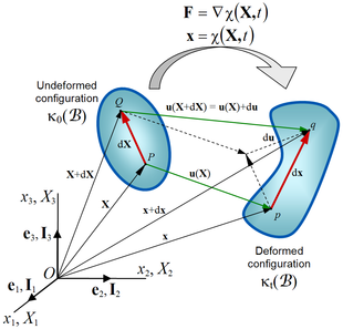
Figure 2. Deformation of a continuum body.

The deformation gradient tensor ${displaystyle mathbf {F} (mathbf {X} ,t)=F_{jK}mathbf {e} _{j}otimes mathbf {I} _{K}}$ is related to both the reference and current configuration, as seen by the unit vectors ${mathbf e}_{j}$ and ${mathbf I}_{K},!$ , therefore it is a two-point tensor.

Due to the assumption of continuity of , has the inverse ${displaystyle mathbf {H} =mathbf {F} ^{-1},!}$ , where is the spatial deformation gradient tensor. Then, by the implicit function theorem,^[1] the Jacobian determinant must be nonsingular, i.e.

The material deformation gradient tensor ${displaystyle mathbf {F} (mathbf {X} ,t)=F_{jK}mathbf {e} _{j}otimes mathbf {I} _{K}}$ is a second-order tensor that represents the gradient of the mapping function or functional relation , which describes the motion of a continuum. The material deformation gradient tensor characterizes the local deformation at a material point with position vector , i.e., deformation at neighbouring points, by transforming (linear transformation) a material line element emanating from that point from the reference configuration to the current or deformed configuration, assuming continuity in the mapping function , i.e. differentiable function of and time t,! , which implies that cracks and voids do not open or close during the deformation. Thus we have,

${displaystyle {begin{aligned}dmathbf {x} &={frac {partial mathbf {x} }{partial mathbf {X} }},dmathbf {X} qquad &{text{or}}&qquad dx_{j}={frac {partial x_{j}}{partial X_{K}}},dX_{K}\&=nabla chi (mathbf {X} ,t),dmathbf {X} qquad &{text{or}}&qquad dx_{j}=F_{jK},dX_{K},.\&=mathbf {F} (mathbf {X} ,t),dmathbf {X} end{aligned}}}$

Relative displacement vector[edit]

Consider a particle or material point with position vector ${displaystyle mathbf {X} =X_{I}mathbf {I} _{I}}$ in the undeformed configuration (Figure 2). After a displacement of the body, the new position of the particle indicated by in the new configuration is given by the vector position ${displaystyle mathbf {x} =x_{i}mathbf {e} _{i},!}$ . The coordinate systems for the undeformed and deformed configuration can be superimposed for convenience.

Consider now a material point neighboring P,! , with position vector ${displaystyle mathbf {X} +Delta mathbf {X} =(X_{I}+Delta X_{I})mathbf {I} _{I},!}$ . In the deformed configuration this particle has a new position given by the position vector . Assuming that the line segments Delta X and joining the particles and in both the undeformed and deformed configuration, respectively, to be very small, then we can express them as and . Thus from Figure 2 we have

${displaystyle {begin{aligned}mathbf {x} +dmathbf {x} &=mathbf {X} +dmathbf {X} +mathbf {u} (mathbf {X} +dmathbf {X} )\dmathbf {x} &=mathbf {X} -mathbf {x} +dmathbf {X} +mathbf {u} (mathbf {X} +dmathbf {X} )\&=dmathbf {X} +mathbf {u} (mathbf {X} +dmathbf {X} )-mathbf {u} (mathbf {X} )\&=dmathbf {X} +dmathbf {u} \end{aligned}}}$

where is the relative displacement vector, which represents the relative displacement of with respect to in the deformed configuration.

Taylor approximation[edit]

For an infinitesimal element , and assuming continuity on the displacement field, it is possible to use a Taylor series expansion around point P,! , neglecting higher-order terms, to approximate the components of the relative displacement vector for the neighboring particle as

${displaystyle {begin{aligned}mathbf {u} (mathbf {X} +dmathbf {X} )&=mathbf {u} (mathbf {X} )+dmathbf {u} quad &{text{or}}&quad u_{i}^{*}=u_{i}+du_{i}\&approx mathbf {u} (mathbf {X} )+nabla _{mathbf {X} }mathbf {u} cdot dmathbf {X} quad &{text{or}}&quad u_{i}^{*}approx u_{i}+{frac {partial u_{i}}{partial X_{J}}}dX_{J},.end{aligned}}}$

Thus, the previous equation can be written as

${displaystyle {begin{aligned}dmathbf {x} &=dmathbf {X} +dmathbf {u} \&=dmathbf {X} +nabla _{mathbf {X} }mathbf {u} cdot dmathbf {X} \&=left(mathbf {I} +nabla _{mathbf {X} }mathbf {u} right)dmathbf {X} \&=mathbf {F} dmathbf {X} end{aligned}}}$

Time-derivative of the deformation gradient[edit]

Calculations that involve the time-dependent deformation of a body often require a time derivative of the deformation gradient to be calculated. A geometrically consistent definition of such a derivative requires an excursion into differential geometry^[2] but we avoid those issues in this article.

The time derivative of is

${displaystyle {dot {mathbf {F} }}={frac {partial mathbf {F} }{partial t}}={frac {partial }{partial t}}left[{frac {partial mathbf {x} (mathbf {X} ,t)}{partial mathbf {X} }}right]={frac {partial }{partial mathbf {X} }}left[{frac {partial mathbf {x} (mathbf {X} ,t)}{partial t}}right]={frac {partial }{partial mathbf {X} }}left[mathbf {V} (mathbf {X} ,t)right]}$

where is the (material) velocity. The derivative on the right hand side represents a material velocity gradient. It is common to convert that into a spatial gradient by applying the chain rule for derivatives, i.e.,

${displaystyle {dot {mathbf {F} }}={frac {partial }{partial mathbf {X} }}left[mathbf {V} (mathbf {X} ,t)right]={frac {partial }{partial mathbf {X} }}left[mathbf {v} (mathbf {x} (mathbf {X} ,t),t)right]=left.{frac {partial }{partial mathbf {x} }}left[mathbf {v} (mathbf {x} ,t)right]right|_{mathbf {x} =mathbf {x} (mathbf {X} ,t)}cdot {frac {partial mathbf {x} (mathbf {X} ,t)}{partial mathbf {X} }}={boldsymbol {l}}cdot mathbf {F} }$

where is the spatial velocity gradient and where is the spatial (Eulerian) velocity at . If the spatial velocity gradient is constant in time, the above equation can be solved exactly to give

${displaystyle mathbf {F} =e^{{boldsymbol {l}},t}}$

assuming at t=0 . There are several methods of computing the exponential above.

Related quantities often used in continuum mechanics are the rate of deformation tensor and the spin tensor defined, respectively, as:

${displaystyle {boldsymbol {d}}={tfrac {1}{2}}left({boldsymbol {l}}+{boldsymbol {l}}^{T}right),,~~{boldsymbol {w}}={tfrac {1}{2}}left({boldsymbol {l}}-{boldsymbol {l}}^{T}right),.}$

The rate of deformation tensor gives the rate of stretching of line elements while the spin tensor indicates the rate of rotation or vorticity of the motion.

The material time derivative of the inverse of the deformation gradient (keeping the reference configuration fixed) is often required in analyses that involve finite strains. This derivative is

${displaystyle {frac {partial }{partial t}}left(mathbf {F} ^{-1}right)=-mathbf {F} ^{-1}cdot {dot {mathbf {F} }}cdot mathbf {F} ^{-1},.}$

The above relation can be verified by taking the material time derivative of ${displaystyle mathbf {F} ^{-1}cdot dmathbf {x} =dmathbf {X} }$ and noting that .

Transformation of a surface and volume element[edit]

To transform quantities that are defined with respect to areas in a deformed configuration to those relative to areas in a reference configuration, and vice versa, we use Nanson’s relation, expressed as

${displaystyle da~mathbf {n} =J~dA~mathbf {F} ^{-T}cdot mathbf {N} }$

where is an area of a region in the deformed configuration, is the same area in the reference configuration, and is the outward normal to the area element in the current configuration while is the outward normal in the reference configuration, is the deformation gradient, and .

The corresponding formula for the transformation of the volume element is

Derivation of Nanson’s relation (see also ^[3])

To see how this formula is derived, we start with the oriented area elements in the reference and current configurations:

The reference and current volumes of an element are

${displaystyle dV=dmathbf {A} ^{T}cdot dmathbf {L} ~;~~dv=dmathbf {a} ^{T}cdot dmathbf {l} }$

where .

Therefore,

${displaystyle dmathbf {a} ^{T}cdot dmathbf {l} =dv=J~dV=J~dmathbf {A} ^{T}cdot dmathbf {L} }$

or,

${displaystyle dmathbf {a} ^{T}cdot mathbf {F} cdot dmathbf {L} =dv=J~dV=J~dmathbf {A} ^{T}cdot dmathbf {L} }$

so,

${displaystyle dmathbf {a} ^{T}cdot mathbf {F} =J~dmathbf {A} ^{T}}$

So we get

${displaystyle dmathbf {a} =J~mathbf {F} ^{-T}cdot dmathbf {A} }$

or,

${displaystyle da~mathbf {n} =J~dA~mathbf {F} ^{-T}cdot mathbf {N} }$

Q.E.D.

Polar decomposition of the deformation gradient tensor[edit]

Figure 3. Representation of the polar decomposition of the deformation gradient

The deformation gradient , like any invertible second-order tensor, can be decomposed, using the polar decomposition theorem, into a product of two second-order tensors (Truesdell and Noll, 1965): an orthogonal tensor and a positive definite symmetric tensor, i.e.,

where the tensor is a proper orthogonal tensor, i.e., ${displaystyle mathbf {R} ^{-1}=mathbf {R} ^{T}}$ and , representing a rotation; the tensor is the right stretch tensor; and the left stretch tensor. The terms right and left means that they are to the right and left of the rotation tensor , respectively. and are both positive definite, i.e. and for all non-zero ${displaystyle mathbf {x} in mathbb {R} ^{3}}$ , and symmetric tensors, i.e. ${displaystyle mathbf {U} =mathbf {U} ^{T}}$ and ${displaystyle mathbf {V} =mathbf {V} ^{T},!}$ , of second order.

This decomposition implies that the deformation of a line element in the undeformed configuration onto in the deformed configuration, i.e., , may be obtained either by first stretching the element by , i.e. , followed by a rotation , i.e., ; or equivalently, by applying a rigid rotation first, i.e., , followed later by a stretching , i.e., (See Figure 3).

Due to the orthogonality of

${displaystyle mathbf {V} =mathbf {R} cdot mathbf {U} cdot mathbf {R} ^{T}}$

so that and have the same eigenvalues or principal stretches, but different eigenvectors or principal directions ${displaystyle mathbf {N} _{i}}$ and ${mathbf {n}}_{i},!$ , respectively. The principal directions are related by

${displaystyle mathbf {n} _{i}=mathbf {R} mathbf {N} _{i}.}$

This polar decomposition, which is unique as is invertible with a positive determinant, is a corollary of the singular-value decomposition.

Deformation tensors[edit]

Several rotation-independent deformation tensors are used in mechanics. In solid mechanics, the most popular of these are the right and left Cauchy–Green deformation tensors.

Since a pure rotation should not induce any strains in a deformable body, it is often convenient to use rotation-independent measures of deformation in continuum mechanics. As a rotation followed by its inverse rotation leads to no change ( $mathbf{R}mathbf{R}^T=mathbf{R}^Tmathbf{R}=mathbf{I},!$ ) we can exclude the rotation by multiplying by its transpose.

The right Cauchy–Green deformation tensor[edit]

In 1839, George Green introduced a deformation tensor known as the right Cauchy–Green deformation tensor or Green’s deformation tensor, defined as:^[4]^[5]

${displaystyle mathbf {C} =mathbf {F} ^{T}mathbf {F} =mathbf {U} ^{2}qquad {text{or}}qquad C_{IJ}=F_{kI}~F_{kJ}={frac {partial x_{k}}{partial X_{I}}}{frac {partial x_{k}}{partial X_{J}}}.}$

Physically, the Cauchy–Green tensor gives us the square of local change in distances due to deformation, i.e. ${displaystyle dmathbf {x} ^{2}=dmathbf {X} cdot mathbf {C} cdot dmathbf {X} }$

Invariants of are often used in the expressions for strain energy density functions. The most commonly used invariants are

${displaystyle {begin{aligned}I_{1}^{C}&:={text{tr}}(mathbf {C} )=C_{II}=lambda _{1}^{2}+lambda _{2}^{2}+lambda _{3}^{2}\I_{2}^{C}&:={tfrac {1}{2}}left[({text{tr}}~mathbf {C} )^{2}-{text{tr}}(mathbf {C} ^{2})right]={tfrac {1}{2}}left[(C_{JJ})^{2}-C_{IK}C_{KI}right]=lambda _{1}^{2}lambda _{2}^{2}+lambda _{2}^{2}lambda _{3}^{2}+lambda _{3}^{2}lambda _{1}^{2}\I_{3}^{C}&:=det(mathbf {C} )=J^{2}=lambda _{1}^{2}lambda _{2}^{2}lambda _{3}^{2}.end{aligned}}}$

where is the determinant of the deformation gradient and $lambda _{i}$ are stretch ratios for the unit fibers that are initially oriented along the eigenvector directions of the right (reference) stretch tensor (these are not generally aligned with the three axis of the coordinate systems).

The Finger deformation tensor[edit]

The IUPAC recommends^[5] that the inverse of the right Cauchy–Green deformation tensor (called the Cauchy tensor in that document), i. e., ${mathbf C}^{{-1}}$ , be called the Finger tensor. However, that nomenclature is not universally accepted in applied mechanics.

${displaystyle mathbf {f} =mathbf {C} ^{-1}=mathbf {F} ^{-1}mathbf {F} ^{-T}qquad {text{or}}qquad f_{IJ}={frac {partial X_{I}}{partial x_{k}}}{frac {partial X_{J}}{partial x_{k}}}}$

The left Cauchy–Green or Finger deformation tensor[edit]

Reversing the order of multiplication in the formula for the right Green–Cauchy deformation tensor leads to the left Cauchy–Green deformation tensor which is defined as:

${displaystyle mathbf {B} =mathbf {F} mathbf {F} ^{T}=mathbf {V} ^{2}qquad {text{or}}qquad B_{ij}={frac {partial x_{i}}{partial X_{K}}}{frac {partial x_{j}}{partial X_{K}}}}$

The left Cauchy–Green deformation tensor is often called the Finger deformation tensor, named after Josef Finger (1894).^[5]^[6]^[7]

Invariants of are also used in the expressions for strain energy density functions. The conventional invariants are defined as

${displaystyle {begin{aligned}I_{1}&:={text{tr}}(mathbf {B} )=B_{ii}=lambda _{1}^{2}+lambda _{2}^{2}+lambda _{3}^{2}\I_{2}&:={tfrac {1}{2}}left[({text{tr}}~mathbf {B} )^{2}-{text{tr}}(mathbf {B} ^{2})right]={tfrac {1}{2}}left(B_{ii}^{2}-B_{jk}B_{kj}right)=lambda _{1}^{2}lambda _{2}^{2}+lambda _{2}^{2}lambda _{3}^{2}+lambda _{3}^{2}lambda _{1}^{2}\I_{3}&:=det mathbf {B} =J^{2}=lambda _{1}^{2}lambda _{2}^{2}lambda _{3}^{2}end{aligned}}}$

where is the determinant of the deformation gradient.

For compressible materials, a slightly different set of invariants is used:

${displaystyle ({bar {I}}_{1}:=J^{-2/3}I_{1}~;~~{bar {I}}_{2}:=J^{-4/3}I_{2}~;~~Jneq 1)~.}$

The Cauchy deformation tensor[edit]

Earlier in 1828,^[8] Augustin-Louis Cauchy introduced a deformation tensor defined as the inverse of the left Cauchy–Green deformation tensor, ${mathbf B}^{{-1}},!$ . This tensor has also been called the Piola tensor^[5] and the Finger tensor^[9] in the rheology and fluid dynamics literature.

${displaystyle mathbf {c} =mathbf {B} ^{-1}=mathbf {F} ^{-T}mathbf {F} ^{-1}qquad {text{or}}qquad c_{ij}={frac {partial X_{K}}{partial x_{i}}}{frac {partial X_{K}}{partial x_{j}}}}$

Spectral representation[edit]

If there are three distinct principal stretches $lambda _{i},!$ , the spectral decompositions of and is given by

${displaystyle mathbf {C} =sum _{i=1}^{3}lambda _{i}^{2}mathbf {N} _{i}otimes mathbf {N} _{i}qquad {text{and}}qquad mathbf {B} =sum _{i=1}^{3}lambda _{i}^{2}mathbf {n} _{i}otimes mathbf {n} _{i}}$

Furthermore,

${displaystyle mathbf {U} =sum _{i=1}^{3}lambda _{i}mathbf {N} _{i}otimes mathbf {N} _{i}~;~~mathbf {V} =sum _{i=1}^{3}lambda _{i}mathbf {n} _{i}otimes mathbf {n} _{i}}$

${displaystyle mathbf {R} =sum _{i=1}^{3}mathbf {n} _{i}otimes mathbf {N} _{i}~;~~mathbf {F} =sum _{i=1}^{3}lambda _{i}mathbf {n} _{i}otimes mathbf {N} _{i}}$

Observe that

${displaystyle mathbf {V} =mathbf {R} ~mathbf {U} ~mathbf {R} ^{T}=sum _{i=1}^{3}lambda _{i}~mathbf {R} ~(mathbf {N} _{i}otimes mathbf {N} _{i})~mathbf {R} ^{T}=sum _{i=1}^{3}lambda _{i}~(mathbf {R} ~mathbf {N} _{i})otimes (mathbf {R} ~mathbf {N} _{i})}$

Therefore, the uniqueness of the spectral decomposition also implies that ${displaystyle mathbf {n} _{i}=mathbf {R} ~mathbf {N} _{i},!}$ . The left stretch () is also called the spatial stretch tensor while the right stretch () is called the material stretch tensor.

The effect of acting on ${displaystyle mathbf {N} _{i}}$ is to stretch the vector by $lambda _{i}$ and to rotate it to the new orientation ${mathbf {n}}_{i},!$ , i.e.,

${displaystyle mathbf {F} ~mathbf {N} _{i}=lambda _{i}~(mathbf {R} ~mathbf {N} _{i})=lambda _{i}~mathbf {n} _{i}}$

In a similar vein,

${displaystyle mathbf {F} ^{-T}~mathbf {N} _{i}={cfrac {1}{lambda _{i}}}~mathbf {n} _{i}~;~~mathbf {F} ^{T}~mathbf {n} _{i}=lambda _{i}~mathbf {N} _{i}~;~~mathbf {F} ^{-1}~mathbf {n} _{i}={cfrac {1}{lambda _{i}}}~mathbf {N} _{i}~.}$

Examples[edit]

Uniaxial extension of an incompressible material: This is the case where a specimen is stretched in 1-direction with a stretch ratio of ${mathbf {alpha =alpha _{1}}},!$ . If the volume remains constant, the contraction in the other two directions is such that ${displaystyle mathbf {alpha _{1}alpha _{2}alpha _{3}=1} }$ or ${mathbf {alpha _{2}=alpha _{3}=alpha ^{{-0.5}}}},!$ . Then:

${displaystyle mathbf {F} ={begin{bmatrix}alpha &0&0\0&alpha ^{-0.5}&0\0&0&alpha ^{-0.5}end{bmatrix}}}$

${displaystyle mathbf {B} =mathbf {C} ={begin{bmatrix}alpha ^{2}&0&0\0&alpha ^{-1}&0\0&0&alpha ^{-1}end{bmatrix}}}$
Simple shear: ${displaystyle mathbf {F} ={begin{bmatrix}1&gamma &0\0&1&0\0&0&1end{bmatrix}}}$

${displaystyle mathbf {B} ={begin{bmatrix}1+gamma ^{2}&gamma &0\gamma &1&0\0&0&1end{bmatrix}}}$

${displaystyle mathbf {C} ={begin{bmatrix}1&gamma &0\gamma &1+gamma ^{2}&0\0&0&1end{bmatrix}}}$
Rigid body rotation: ${displaystyle mathbf {F} ={begin{bmatrix}cos theta &sin theta &0\-sin theta &cos theta &0\0&0&1end{bmatrix}}}$

${displaystyle mathbf {B} =mathbf {C} ={begin{bmatrix}1&0&0\0&1&0\0&0&1end{bmatrix}}=mathbf {1} }$

Derivatives of stretch[edit]

Derivatives of the stretch with respect to the right Cauchy–Green deformation tensor are used to derive the stress-strain relations of many solids, particularly hyperelastic materials. These derivatives are

${displaystyle {cfrac {partial lambda _{i}}{partial mathbf {C} }}={cfrac {1}{2lambda _{i}}}~mathbf {N} _{i}otimes mathbf {N} _{i}={cfrac {1}{2lambda _{i}}}~mathbf {R} ^{T}~(mathbf {n} _{i}otimes mathbf {n} _{i})~mathbf {R} ~;~~i=1,2,3}$

and follow from the observations that

${displaystyle mathbf {C} :(mathbf {N} _{i}otimes mathbf {N} _{i})=lambda _{i}^{2}~;~~~~{cfrac {partial mathbf {C} }{partial mathbf {C} }}={mathsf {I}}^{(s)}~;~~~~{mathsf {I}}^{(s)}:(mathbf {N} _{i}otimes mathbf {N} _{i})=mathbf {N} _{i}otimes mathbf {N} _{i}.}$

Physical interpretation of deformation tensors[edit]

Let ${mathbf {X}}=X^{i}~{boldsymbol {E}}_{i}$ be a Cartesian coordinate system defined on the undeformed body and let ${mathbf {x}}=x^{i}~{boldsymbol {E}}_{i}$ be another system defined on the deformed body. Let a curve in the undeformed body be parametrized using . Its image in the deformed body is .

The undeformed length of the curve is given by

${displaystyle l_{X}=int _{0}^{1}left|{cfrac {dmathbf {X} }{ds}}right|~ds=int _{0}^{1}{sqrt {{cfrac {dmathbf {X} }{ds}}cdot {cfrac {dmathbf {X} }{ds}}}}~ds=int _{0}^{1}{sqrt {{cfrac {dmathbf {X} }{ds}}cdot {boldsymbol {I}}cdot {cfrac {dmathbf {X} }{ds}}}}~ds}$

After deformation, the length becomes

${displaystyle {begin{aligned}l_{x}&=int _{0}^{1}left|{cfrac {dmathbf {x} }{ds}}right|~ds=int _{0}^{1}{sqrt {{cfrac {dmathbf {x} }{ds}}cdot {cfrac {dmathbf {x} }{ds}}}}~ds=int _{0}^{1}{sqrt {left({cfrac {dmathbf {x} }{dmathbf {X} }}cdot {cfrac {dmathbf {X} }{ds}}right)cdot left({cfrac {dmathbf {x} }{dmathbf {X} }}cdot {cfrac {dmathbf {X} }{ds}}right)}}~ds\&=int _{0}^{1}{sqrt {{cfrac {dmathbf {X} }{ds}}cdot left[left({cfrac {dmathbf {x} }{dmathbf {X} }}right)^{T}cdot {cfrac {dmathbf {x} }{dmathbf {X} }}right]cdot {cfrac {dmathbf {X} }{ds}}}}~dsend{aligned}}}$

Note that the right Cauchy–Green deformation tensor is defined as

${displaystyle {boldsymbol {C}}:={boldsymbol {F}}^{T}cdot {boldsymbol {F}}=left({cfrac {dmathbf {x} }{dmathbf {X} }}right)^{T}cdot {cfrac {dmathbf {x} }{dmathbf {X} }}}$

Hence,

${displaystyle l_{x}=int _{0}^{1}{sqrt {{cfrac {dmathbf {X} }{ds}}cdot {boldsymbol {C}}cdot {cfrac {dmathbf {X} }{ds}}}}~ds}$

which indicates that changes in length are characterized by .

Finite strain tensors[edit]

The concept of strain is used to evaluate how much a given displacement differs locally from a rigid body displacement.^[1]^[10]^[11] One of such strains for large deformations is the Lagrangian finite strain tensor, also called the Green-Lagrangian strain tensor or Green – St-Venant strain tensor, defined as

${displaystyle mathbf {E} ={frac {1}{2}}(mathbf {C} -mathbf {I} )qquad {text{or}}qquad E_{KL}={frac {1}{2}}left({frac {partial x_{j}}{partial X_{K}}}{frac {partial x_{j}}{partial X_{L}}}-delta _{KL}right)}$

or as a function of the displacement gradient tensor

${displaystyle mathbf {E} ={frac {1}{2}}left[(nabla _{mathbf {X} }mathbf {u} )^{T}+nabla _{mathbf {X} }mathbf {u} +(nabla _{mathbf {X} }mathbf {u} )^{T}cdot nabla _{mathbf {X} }mathbf {u} right]}$

${displaystyle E_{KL}={frac {1}{2}}left({frac {partial u_{K}}{partial X_{L}}}+{frac {partial u_{L}}{partial X_{K}}}+{frac {partial u_{M}}{partial X_{K}}}{frac {partial u_{M}}{partial X_{L}}}right)}$

The Green-Lagrangian strain tensor is a measure of how much differs from .

The Eulerian-Almansi finite strain tensor, referenced to the deformed configuration, i.e. Eulerian description, is defined as

${displaystyle mathbf {e} ={frac {1}{2}}(mathbf {I} -mathbf {c} )={frac {1}{2}}(mathbf {I} -mathbf {B} ^{-1})qquad {text{or}}qquad e_{rs}={frac {1}{2}}left(delta _{rs}-{frac {partial X_{M}}{partial x_{r}}}{frac {partial X_{M}}{partial x_{s}}}right)}$

or as a function of the displacement gradients we have

${displaystyle e_{ij}={frac {1}{2}}left({frac {partial u_{i}}{partial x_{j}}}+{frac {partial u_{j}}{partial x_{i}}}-{frac {partial u_{k}}{partial x_{i}}}{frac {partial u_{k}}{partial x_{j}}}right)}$

Derivation of the Lagrangian and Eulerian finite strain tensors

A measure of deformation is the difference between the squares of the differential line element , in the undeformed configuration, and , in the deformed configuration (Figure 2). Deformation has occurred if the difference is non zero, otherwise a rigid-body displacement has occurred. Thus we have,

${displaystyle dmathbf {x} ^{2}-dmathbf {X} ^{2}=dmathbf {x} cdot dmathbf {x} -dmathbf {X} cdot dmathbf {X} qquad {text{or}}qquad (dx)^{2}-(dX)^{2}=dx_{j}dx_{j}-dX_{M},dX_{M}}$

In the Lagrangian description, using the material coordinates as the frame of reference, the linear transformation between the differential lines is

${displaystyle dmathbf {x} ={frac {partial mathbf {x} }{partial mathbf {X} }},dmathbf {X} =mathbf {F} ,dmathbf {X} qquad {text{or}}qquad dx_{j}={frac {partial x_{j}}{partial X_{M}}},dX_{M}}$

Then we have,

${displaystyle {begin{aligned}dmathbf {x} ^{2}&=dmathbf {x} cdot dmathbf {x} \&=mathbf {F} cdot dmathbf {X} cdot mathbf {F} cdot dmathbf {X} \&=dmathbf {X} cdot mathbf {F} ^{T}mathbf {F} cdot dmathbf {X} \&=dmathbf {X} cdot mathbf {C} cdot dmathbf {X} end{aligned}}qquad {text{or}}qquad {begin{aligned}(dx)^{2}&=dx_{j},dx_{j}\&={frac {partial x_{j}}{partial X_{K}}}{frac {partial x_{j}}{partial X_{L}}},dX_{K},dX_{L}\&=C_{KL},dX_{K},dX_{L}\end{aligned}}}$

where ${displaystyle C_{KL}}$ are the components of the right Cauchy–Green deformation tensor, ${displaystyle mathbf {C} =mathbf {F} ^{T}mathbf {F} ,!}$ . Then, replacing this equation into the first equation we have,

${displaystyle {begin{aligned}dmathbf {x} ^{2}-dmathbf {X} ^{2}&=dmathbf {X} cdot mathbf {C} cdot dmathbf {X} -dmathbf {X} cdot dmathbf {X} \&=dmathbf {X} cdot (mathbf {C} -mathbf {I} )cdot dmathbf {X} \&=dmathbf {X} cdot 2mathbf {E} cdot dmathbf {X} \end{aligned}}}$

${displaystyle {begin{aligned}(dx)^{2}-(dX)^{2}&={frac {partial x_{j}}{partial X_{K}}}{frac {partial x_{j}}{partial X_{L}}},dX_{K},dX_{L}-dX_{M},dX_{M}\&=left({frac {partial x_{j}}{partial X_{K}}}{frac {partial x_{j}}{partial X_{L}}}-delta _{KL}right),dX_{K},dX_{L}\&=2E_{KL},dX_{K},dX_{L}end{aligned}}}$

where $E_{{KL}},!$ , are the components of a second-order tensor called the Green – St-Venant strain tensor or the Lagrangian finite strain tensor,

In the Eulerian description, using the spatial coordinates as the frame of reference, the linear transformation between the differential lines is

${displaystyle dmathbf {X} ={frac {partial mathbf {X} }{partial mathbf {x} }}dmathbf {x} =mathbf {F} ^{-1},dmathbf {x} =mathbf {H} ,dmathbf {x} qquad {text{or}}qquad dX_{M}={frac {partial X_{M}}{partial x_{n}}},dx_{n}}$

where ${displaystyle {frac {partial X_{M}}{partial x_{n}}}}$ are the components of the spatial deformation gradient tensor, . Thus we have

${displaystyle {begin{aligned}dmathbf {X} ^{2}&=dmathbf {X} cdot dmathbf {X} \&=mathbf {F} ^{-1}cdot dmathbf {x} cdot mathbf {F} ^{-1}cdot dmathbf {x} \&=dmathbf {x} cdot mathbf {F} ^{-T}mathbf {F} ^{-1}cdot dmathbf {x} \&=dmathbf {x} cdot mathbf {c} cdot dmathbf {x} end{aligned}}qquad {text{or}}qquad {begin{aligned}(dX)^{2}&=dX_{M},dX_{M}\&={frac {partial X_{M}}{partial x_{r}}}{frac {partial X_{M}}{partial x_{s}}},dx_{r},dx_{s}\&=c_{rs},dx_{r},dx_{s}\end{aligned}}}$

where the second order tensor $c_{rs}$ is called Cauchy’s deformation tensor, ${mathbf c}={mathbf F}^{{-T}}{mathbf F}^{{-1}},!$ . Then we have,

${displaystyle {begin{aligned}dmathbf {x} ^{2}-dmathbf {X} ^{2}&=dmathbf {x} cdot dmathbf {x} -dmathbf {x} cdot mathbf {c} cdot dmathbf {x} \&=dmathbf {x} cdot (mathbf {I} -mathbf {c} )cdot dmathbf {x} \&=dmathbf {x} cdot 2mathbf {e} cdot dmathbf {x} \end{aligned}}}$

${displaystyle {begin{aligned}(dx)^{2}-(dX)^{2}&=dx_{j},dx_{j}-{frac {partial X_{M}}{partial x_{r}}}{frac {partial X_{M}}{partial x_{s}}},dx_{r},dx_{s}\&=left(delta _{rs}-{frac {partial X_{M}}{partial x_{r}}}{frac {partial X_{M}}{partial x_{s}}}right),dx_{r},dx_{s}\&=2e_{rs},dx_{r},dx_{s}end{aligned}}}$

where $e_{{rs}},!$ , are the components of a second-order tensor called the Eulerian-Almansi finite strain tensor,

${displaystyle mathbf {e} ={frac {1}{2}}(mathbf {I} -mathbf {c} )qquad {text{or}}qquad e_{rs}={frac {1}{2}}left(delta _{rs}-{frac {partial X_{M}}{partial x_{r}}}{frac {partial X_{M}}{partial x_{s}}}right)}$

Both the Lagrangian and Eulerian finite strain tensors can be conveniently expressed in terms of the displacement gradient tensor. For the Lagrangian strain tensor, first we differentiate the displacement vector with respect to the material coordinates $X_{M}$ to obtain the material displacement gradient tensor, ${displaystyle nabla _{mathbf {X} }mathbf {u} }$

${displaystyle {begin{aligned}mathbf {u} (mathbf {X} ,t)&=mathbf {x} (mathbf {X} ,t)-mathbf {X} \nabla _{mathbf {X} }mathbf {u} &=mathbf {F} -mathbf {I} \mathbf {F} &=nabla _{mathbf {X} }mathbf {u} +mathbf {I} \end{aligned}}qquad {text{or}}qquad {begin{aligned}u_{i}&=x_{i}-delta _{iJ}X_{J}\delta _{iJ}U_{J}&=x_{i}-delta _{iJ}X_{J}\x_{i}&=delta _{iJ}left(U_{J}+X_{J}right)\{frac {partial x_{i}}{partial X_{K}}}&=delta _{iJ}left({frac {partial U_{J}}{partial X_{K}}}+delta _{JK}right)\end{aligned}}}$

Replacing this equation into the expression for the Lagrangian finite strain tensor we have

${displaystyle {begin{aligned}mathbf {E} &={frac {1}{2}}left(mathbf {F} ^{T}mathbf {F} -mathbf {I} right)\&={frac {1}{2}}left[left{(nabla _{mathbf {X} }mathbf {u} )^{T}+mathbf {I} right}left(nabla _{mathbf {X} }mathbf {u} +mathbf {I} right)-mathbf {I} right]\&={frac {1}{2}}left[(nabla _{mathbf {X} }mathbf {u} )^{T}+nabla _{mathbf {X} }mathbf {u} +(nabla _{mathbf {X} }mathbf {u} )^{T}cdot nabla _{mathbf {X} }mathbf {u} right]\end{aligned}}}$

${displaystyle {begin{aligned}E_{KL}&={frac {1}{2}}left({frac {partial x_{j}}{partial X_{K}}}{frac {partial x_{j}}{partial X_{L}}}-delta _{KL}right)\&={frac {1}{2}}left[delta _{jM}left({frac {partial U_{M}}{partial X_{K}}}+delta _{MK}right)delta _{jN}left({frac {partial U_{N}}{partial X_{L}}}+delta _{NL}right)-delta _{KL}right]\&={frac {1}{2}}left[delta _{MN}left({frac {partial U_{M}}{partial X_{K}}}+delta _{MK}right)left({frac {partial U_{N}}{partial X_{L}}}+delta _{NL}right)-delta _{KL}right]\&={frac {1}{2}}left[left({frac {partial U_{M}}{partial X_{K}}}+delta _{MK}right)left({frac {partial U_{M}}{partial X_{L}}}+delta _{ML}right)-delta _{KL}right]\&={frac {1}{2}}left({frac {partial U_{K}}{partial X_{L}}}+{frac {partial U_{L}}{partial X_{K}}}+{frac {partial U_{M}}{partial X_{K}}}{frac {partial U_{M}}{partial X_{L}}}right)end{aligned}}}$

Similarly, the Eulerian-Almansi finite strain tensor can be expressed as

${displaystyle e_{ij}={frac {1}{2}}left({frac {partial u_{i}}{partial x_{j}}}+{frac {partial u_{j}}{partial x_{i}}}-{frac {partial u_{k}}{partial x_{i}}}{frac {partial u_{k}}{partial x_{j}}}right)}$

Seth–Hill family of generalized strain tensors[edit]

B. R. Seth from the Indian Institute of Technology Kharagpur was the first to show that the Green and Almansi strain tensors are special cases of a more general strain measure.^[12]^[13] The idea was further expanded upon by Rodney Hill in 1968.^[14] The Seth–Hill family of strain measures (also called Doyle-Ericksen tensors)^[15] can be expressed as

${displaystyle mathbf {E} _{(m)}={frac {1}{2m}}(mathbf {U} ^{2m}-mathbf {I} )={frac {1}{2m}}left[mathbf {C} ^{m}-mathbf {I} right]}$

For different values of we have:

Green-Lagrangian strain tensor

${displaystyle mathbf {E} _{(1)}={frac {1}{2}}(mathbf {U} ^{2}-mathbf {I} )={frac {1}{2}}(mathbf {C} -mathbf {I} )}$
Biot strain tensor

${displaystyle mathbf {E} _{(1/2)}=(mathbf {U} -mathbf {I} )=mathbf {C} ^{1/2}-mathbf {I} }$
Logarithmic strain, Natural strain, True strain, or Hencky strain

${displaystyle mathbf {E} _{(0)}=ln mathbf {U} ={frac {1}{2}},ln mathbf {C} }$
Almansi strain

${displaystyle mathbf {E} _{(-1)}={frac {1}{2}}left[mathbf {I} -mathbf {U} ^{-2}right]}$

The second-order approximation of these tensors is

${displaystyle mathbf {E} _{(m)}={boldsymbol {varepsilon }}+{tfrac {1}{2}}(nabla mathbf {u} )^{T}cdot nabla mathbf {u} -(1-m){boldsymbol {varepsilon }}^{T}cdot {boldsymbol {varepsilon }}}$

where is the infinitesimal strain tensor.

Many other different definitions of tensors are admissible, provided that they all satisfy the conditions that:^[16]

An example is the set of tensors

${displaystyle mathbf {E} ^{(n)}=left({mathbf {U} }^{n}-{mathbf {U} }^{-n}right)/2n}$

which do not belong to the Seth–Hill class, but have the same 2nd-order approximation as the Seth–Hill measures at m=0 for any value of .^[17]

Stretch ratio[edit]

The stretch ratio is a measure of the extensional or normal strain of a differential line element, which can be defined at either the undeformed configuration or the deformed configuration.

The stretch ratio for the differential element (Figure) in the direction of the unit vector at the material point P,! , in the undeformed configuration, is defined as

${displaystyle Lambda _{(mathbf {N} )}={frac {dx}{dX}}}$

where is the deformed magnitude of the differential element .

Similarly, the stretch ratio for the differential element (Figure), in the direction of the unit vector at the material point p,! , in the deformed configuration, is defined as

${displaystyle {frac {1}{Lambda _{(mathbf {n} )}}}={frac {dX}{dx}}.}$

The normal strain ${displaystyle e_{mathbf {N} }}$ in any direction can be expressed as a function of the stretch ratio,

${displaystyle e_{(mathbf {N} )}={frac {dx-dX}{dX}}=Lambda _{(mathbf {N} )}-1.}$

This equation implies that the normal strain is zero, i.e. no deformation, when the stretch is equal to unity. Some materials, such as elastometers can sustain stretch ratios of 3 or 4 before they fail, whereas traditional engineering materials, such as concrete or steel, fail at much lower stretch ratios, perhaps of the order of 1.1 (reference?)

Physical interpretation of the finite strain tensor[edit]

The diagonal components ${displaystyle E_{KL}}$ of the Lagrangian finite strain tensor are related to the normal strain, e.g.

${displaystyle E_{11}=e_{(mathbf {I} _{1})}+{frac {1}{2}}e_{(mathbf {I} _{1})}^{2}}$

where ${displaystyle e_{(mathbf {I} _{1})}}$ is the normal strain or engineering strain in the direction ${mathbf I}_{1},!$ .

The off-diagonal components ${displaystyle E_{KL}}$ of the Lagrangian finite strain tensor are related to shear strain, e.g.

${displaystyle E_{12}={frac {1}{2}}{sqrt {2E_{11}+1}}{sqrt {2E_{22}+1}}sin phi _{12}}$

where ${displaystyle phi _{12}}$ is the change in the angle between two line elements that were originally perpendicular with directions ${displaystyle mathbf {I} _{1}}$ and ${mathbf I}_{2},!$ , respectively.

Under certain circumstances, i.e. small displacements and small displacement rates, the components of the Lagrangian finite strain tensor may be approximated by the components of the infinitesimal strain tensor

Derivation of the physical interpretation of the Lagrangian and Eulerian finite strain tensors

The stretch ratio for the differential element (Figure) in the direction of the unit vector at the material point P,! , in the undeformed configuration, is defined as

${displaystyle Lambda _{(mathbf {N} )}={frac {dx}{dX}}}$

where is the deformed magnitude of the differential element .

Similarly, the stretch ratio for the differential element (Figure), in the direction of the unit vector at the material point p,! , in the deformed configuration, is defined as

${displaystyle {frac {1}{Lambda _{(mathbf {n} )}}}={frac {dX}{dx}}}$

The square of the stretch ratio is defined as

${displaystyle Lambda _{(mathbf {N} )}^{2}=left({frac {dx}{dX}}right)^{2}}$

Knowing that

${displaystyle (dx)^{2}=C_{KL}dX_{K}dX_{L}}$

we have

${displaystyle Lambda _{(mathbf {N} )}^{2}=C_{KL}N_{K}N_{L}}$

where ${displaystyle N_{K}}$ and ${displaystyle N_{L}}$ are unit vectors.

The normal strain or engineering strain ${displaystyle e_{mathbf {N} }}$ in any direction can be expressed as a function of the stretch ratio,

${displaystyle e_{(mathbf {N} )}={frac {dx-dX}{dX}}=Lambda _{(mathbf {N} )}-1}$

Thus, the normal strain in the direction ${displaystyle mathbf {I} _{1}}$ at the material point may be expressed in terms of the stretch ratio as

${displaystyle {begin{aligned}e_{(mathbf {I} _{1})}={frac {dx_{1}-dX_{1}}{dX_{1}}}&=Lambda _{(mathbf {I} _{1})}-1\&={sqrt {C_{11}}}-1={sqrt {delta _{11}+2E_{11}}}-1\&={sqrt {1+2E_{11}}}-1end{aligned}}}$

solving for ${displaystyle E_{11}}$ we have

${displaystyle {begin{aligned}2E_{11}&={frac {(dx_{1})^{2}-(dX_{1})^{2}}{(dX_{1})^{2}}}\E_{11}&=left({frac {dx_{1}-dX_{1}}{dX_{1}}}right)+{frac {1}{2}}left({frac {dx_{1}-dX_{1}}{dX_{1}}}right)^{2}\&=e_{(mathbf {I} _{1})}+{frac {1}{2}}e_{(mathbf {I} _{1})}^{2}end{aligned}}}$

The shear strain, or change in angle between two line elements ${displaystyle dmathbf {X} _{1}}$ and ${displaystyle dmathbf {X} _{2}}$ initially perpendicular, and oriented in the principal directions ${displaystyle mathbf {I} _{1}}$ and ${mathbf I}_{2},!$ , respectively, can also be expressed as a function of the stretch ratio. From the dot product between the deformed lines ${displaystyle dmathbf {x} _{1}}$ and ${displaystyle dmathbf {x} _{2}}$ we have

${displaystyle {begin{aligned}dmathbf {x} _{1}cdot dmathbf {x} _{2}&=dx_{1}dx_{2}cos theta _{12}\mathbf {F} cdot dmathbf {X} _{1}cdot mathbf {F} cdot dmathbf {X} _{2}&={sqrt {dmathbf {X} _{1}cdot mathbf {F} ^{T}cdot mathbf {F} cdot dmathbf {X} _{1}}}cdot {sqrt {dmathbf {X} _{2}cdot mathbf {F} ^{T}cdot mathbf {F} cdot dmathbf {X} _{2}}}cos theta _{12}\{frac {dmathbf {X} _{1}cdot mathbf {F} ^{T}cdot mathbf {F} cdot dmathbf {X} _{2}}{dX_{1}dX_{2}}}&={frac {{sqrt {dmathbf {X} _{1}cdot mathbf {F} ^{T}cdot mathbf {F} cdot dmathbf {X} _{1}}}cdot {sqrt {dmathbf {X} _{2}cdot mathbf {F} ^{T}cdot mathbf {F} cdot dmathbf {X} _{2}}}}{dX_{1}dX_{2}}}cos theta _{12}\mathbf {I} _{1}cdot mathbf {C} cdot mathbf {I} _{2}&=Lambda _{mathbf {I} _{1}}Lambda _{mathbf {I} _{2}}cos theta _{12}end{aligned}}}$

where ${displaystyle theta _{12}}$ is the angle between the lines ${displaystyle dmathbf {x} _{1}}$ and ${displaystyle dmathbf {x} _{2}}$ in the deformed configuration. Defining ${displaystyle phi _{12}}$ as the shear strain or reduction in the angle between two line elements that were originally perpendicular, we have

${displaystyle phi _{12}={frac {pi }{2}}-theta _{12}}$

thus,

${displaystyle cos theta _{12}=sin phi _{12}}$

then

${displaystyle mathbf {I} _{1}cdot mathbf {C} cdot mathbf {I} _{2}=Lambda _{mathbf {I} _{1}}Lambda _{mathbf {I} _{2}}sin phi _{12}}$

${displaystyle {begin{aligned}C_{12}&={sqrt {C_{11}}}{sqrt {C_{22}}}sin phi _{12}\2E_{12}+delta _{12}&={sqrt {2E_{11}+1}}{sqrt {2E_{22}+1}}sin phi _{12}\E_{12}&={frac {1}{2}}{sqrt {2E_{11}+1}}{sqrt {2E_{22}+1}}sin phi _{12}end{aligned}}}$

Deformation tensors in convected curvilinear coordinates[edit]

A representation of deformation tensors in curvilinear coordinates is useful for many problems in continuum mechanics such as nonlinear shell theories and large plastic deformations. Let ${mathbf {x}}={mathbf {x}}(xi ^{1},xi ^{2},xi ^{3})$ denote the function by which a position vector in space is constructed from coordinates $(xi ^{1},xi ^{2},xi ^{3})$ . The coordinates are said to be «convected» if they correspond to a one-to-one mapping to and from Lagrangian particles in a continuum body. If the coordinate grid is «painted» on the body in its initial configuration, then this grid will deform and flow with the motion of material to remain painted on the same material particles in the deformed configuration so that grid lines intersect at the same material particle in either configuration. The tangent vector to the deformed coordinate grid line curve $xi ^{i}$ at is given by

${displaystyle mathbf {g} _{i}={frac {partial mathbf {x} }{partial xi ^{i}}}}$

The three tangent vectors at form a local basis. These vectors are related the reciprocal basis vectors by

${displaystyle mathbf {g} _{i}cdot mathbf {g} ^{j}=delta _{i}^{j}}$

Let us define a second-order tensor field (also called the metric tensor) with components

${displaystyle g_{ij}:={frac {partial mathbf {x} }{partial xi ^{i}}}cdot {frac {partial mathbf {x} }{partial xi ^{j}}}=mathbf {g} _{i}cdot mathbf {g} _{j}}$

The Christoffel symbols of the first kind can be expressed as

${displaystyle Gamma _{ijk}={tfrac {1}{2}}[(mathbf {g} _{i}cdot mathbf {g} _{k})_{,j}+(mathbf {g} _{j}cdot mathbf {g} _{k})_{,i}-(mathbf {g} _{i}cdot mathbf {g} _{j})_{,k}]}$

To see how the Christoffel symbols are related to the Right Cauchy–Green deformation tensor let us similarly define two bases, the already mentioned one that is tangent to deformed grid lines and another that is tangent to the undeformed grid lines. Namely,

${displaystyle mathbf {G} _{i}:={frac {partial mathbf {X} }{partial xi ^{i}}}~;~~mathbf {G} _{i}cdot mathbf {G} ^{j}=delta _{i}^{j}~;~~mathbf {g} _{i}:={frac {partial mathbf {x} }{partial xi ^{i}}}~;~~mathbf {g} _{i}cdot mathbf {g} ^{j}=delta _{i}^{j}}$

The deformation gradient in curvilinear coordinates[edit]

Using the definition of the gradient of a vector field in curvilinear coordinates, the deformation gradient can be written as

${displaystyle {boldsymbol {F}}={boldsymbol {nabla }}_{mathbf {X} }mathbf {x} ={frac {partial mathbf {x} }{partial xi ^{i}}}otimes mathbf {G} ^{i}=mathbf {g} _{i}otimes mathbf {G} ^{i}}$

The right Cauchy–Green tensor in curvilinear coordinates[edit]

The right Cauchy–Green deformation tensor is given by

${displaystyle {boldsymbol {C}}={boldsymbol {F}}^{T}cdot {boldsymbol {F}}=(mathbf {G} ^{i}otimes mathbf {g} _{i})cdot (mathbf {g} _{j}otimes mathbf {G} ^{j})=(mathbf {g} _{i}cdot mathbf {g} _{j})(mathbf {G} ^{i}otimes mathbf {G} ^{j})}$

If we express in terms of components with respect to the basis { ${mathbf {G}}^{i}$ } we have

${displaystyle {boldsymbol {C}}=C_{ij}~mathbf {G} ^{i}otimes mathbf {G} ^{j}}$

Therefore,

${displaystyle C_{ij}=mathbf {g} _{i}cdot mathbf {g} _{j}=g_{ij}}$

and the corresponding Christoffel symbol of the first kind may be written in the following form.

${displaystyle Gamma _{ijk}={tfrac {1}{2}}[C_{ik,j}+C_{jk,i}-C_{ij,k}]={tfrac {1}{2}}[(mathbf {G} _{i}cdot {boldsymbol {C}}cdot mathbf {G} _{k})_{,j}+(mathbf {G} _{j}cdot {boldsymbol {C}}cdot mathbf {G} _{k})_{,i}-(mathbf {G} _{i}cdot {boldsymbol {C}}cdot mathbf {G} _{j})_{,k}]}$

Some relations between deformation measures and Christoffel symbols[edit]

Consider a one-to-one mapping from ${mathbf {X}}={X^{1},X^{2},X^{3}}$ to ${mathbf {x}}={x^{1},x^{2},x^{3}}$ and let us assume that there exist two positive-definite, symmetric second-order tensor fields and that satisfy

${displaystyle G_{ij}={frac {partial X^{alpha }}{partial x^{i}}}~{frac {partial X^{beta }}{partial x^{j}}}~g_{alpha beta }}$

Then,

${displaystyle {frac {partial G_{ij}}{partial x^{k}}}=left({frac {partial ^{2}X^{alpha }}{partial x^{i}partial x^{k}}}~{frac {partial X^{beta }}{partial x^{j}}}+{frac {partial X^{alpha }}{partial x^{i}}}~{frac {partial ^{2}X^{beta }}{partial x^{j}partial x^{k}}}right)~g_{alpha beta }+{frac {partial X^{alpha }}{partial x^{i}}}~{frac {partial X^{beta }}{partial x^{j}}}~{frac {partial g_{alpha beta }}{partial x^{k}}}}$

Noting that

${displaystyle {frac {partial g_{alpha beta }}{partial x^{k}}}={frac {partial X^{gamma }}{partial x^{k}}}~{frac {partial g_{alpha beta }}{partial X^{gamma }}}}$

and $g_{{alpha beta }}=g_{{beta alpha }}$ we have

${displaystyle {begin{aligned}{frac {partial G_{ij}}{partial x^{k}}}&=left({frac {partial ^{2}X^{alpha }}{partial x^{i}partial x^{k}}}~{frac {partial X^{beta }}{partial x^{j}}}+{frac {partial ^{2}X^{alpha }}{partial x^{j}partial x^{k}}}~{frac {partial X^{beta }}{partial x^{i}}}right)~g_{alpha beta }+{frac {partial X^{alpha }}{partial x^{i}}}~{frac {partial X^{beta }}{partial x^{j}}}~{frac {partial X^{gamma }}{partial x^{k}}}~{frac {partial g_{alpha beta }}{partial X^{gamma }}}\{frac {partial G_{ik}}{partial x^{j}}}&=left({frac {partial ^{2}X^{alpha }}{partial x^{i}partial x^{j}}}~{frac {partial X^{beta }}{partial x^{k}}}+{frac {partial ^{2}X^{alpha }}{partial x^{j}partial x^{k}}}~{frac {partial X^{beta }}{partial x^{i}}}right)~g_{alpha beta }+{frac {partial X^{alpha }}{partial x^{i}}}~{frac {partial X^{beta }}{partial x^{k}}}~{frac {partial X^{gamma }}{partial x^{j}}}~{frac {partial g_{alpha beta }}{partial X^{gamma }}}\{frac {partial G_{jk}}{partial x^{i}}}&=left({frac {partial ^{2}X^{alpha }}{partial x^{i}partial x^{j}}}~{frac {partial X^{beta }}{partial x^{k}}}+{frac {partial ^{2}X^{alpha }}{partial x^{i}partial x^{k}}}~{frac {partial X^{beta }}{partial x^{j}}}right)~g_{alpha beta }+{frac {partial X^{alpha }}{partial x^{j}}}~{frac {partial X^{beta }}{partial x^{k}}}~{frac {partial X^{gamma }}{partial x^{i}}}~{frac {partial g_{alpha beta }}{partial X^{gamma }}}end{aligned}}}$

Define

${displaystyle {begin{aligned}_{(x)}Gamma _{ijk}&:={frac {1}{2}}left({frac {partial G_{ik}}{partial x^{j}}}+{frac {partial G_{jk}}{partial x^{i}}}-{frac {partial G_{ij}}{partial x^{k}}}right)\_{(X)}Gamma _{alpha beta gamma }&:={frac {1}{2}}left({frac {partial g_{alpha gamma }}{partial X^{beta }}}+{frac {partial g_{beta gamma }}{partial X^{alpha }}}-{frac {partial g_{alpha beta }}{partial X^{gamma }}}right)\end{aligned}}}$

Hence

${displaystyle _{(x)}Gamma _{ijk}={frac {partial X^{alpha }}{partial x^{i}}}~{frac {partial X^{beta }}{partial x^{j}}}~{frac {partial X^{gamma }}{partial x^{k}}},_{(X)}Gamma _{alpha beta gamma }+{frac {partial ^{2}X^{alpha }}{partial x^{i}partial x^{j}}}~{frac {partial X^{beta }}{partial x^{k}}}~g_{alpha beta }}$

Define

${displaystyle [G^{ij}]=[G_{ij}]^{-1}~;~~[g^{alpha beta }]=[g_{alpha beta }]^{-1}}$

Then

${displaystyle G^{ij}={frac {partial x^{i}}{partial X^{alpha }}}~{frac {partial x^{j}}{partial X^{beta }}}~g^{alpha beta }}$

Define the Christoffel symbols of the second kind as

${displaystyle _{(x)}Gamma _{ij}^{m}:=G^{mk},_{(x)}Gamma _{ijk}~;~~_{(X)}Gamma _{alpha beta }^{nu }:=g^{nu gamma },_{(X)}Gamma _{alpha beta gamma }}$

Then

${displaystyle {begin{aligned}_{(x)}Gamma _{ij}^{m}&=G^{mk}~{frac {partial X^{alpha }}{partial x^{i}}}~{frac {partial X^{beta }}{partial x^{j}}}~{frac {partial X^{gamma }}{partial x^{k}}},_{(X)}Gamma _{alpha beta gamma }+G^{mk}~{frac {partial ^{2}X^{alpha }}{partial x^{i}partial x^{j}}}~{frac {partial X^{beta }}{partial x^{k}}}~g_{alpha beta }\&={frac {partial x^{m}}{partial X^{nu }}}~{frac {partial x^{k}}{partial X^{rho }}}~g^{nu rho }~{frac {partial X^{alpha }}{partial x^{i}}}~{frac {partial X^{beta }}{partial x^{j}}}~{frac {partial X^{gamma }}{partial x^{k}}},_{(X)}Gamma _{alpha beta gamma }+{frac {partial x^{m}}{partial X^{nu }}}~{frac {partial x^{k}}{partial X^{rho }}}~g^{nu rho }~{frac {partial ^{2}X^{alpha }}{partial x^{i}partial x^{j}}}~{frac {partial X^{beta }}{partial x^{k}}}~g_{alpha beta }\&={frac {partial x^{m}}{partial X^{nu }}}~delta _{rho }^{gamma }~g^{nu rho }~{frac {partial X^{alpha }}{partial x^{i}}}~{frac {partial X^{beta }}{partial x^{j}}},_{(X)}Gamma _{alpha beta gamma }+{frac {partial x^{m}}{partial X^{nu }}}~delta _{rho }^{beta }~g^{nu rho }~{frac {partial ^{2}X^{alpha }}{partial x^{i}partial x^{j}}}~g_{alpha beta }\&={frac {partial x^{m}}{partial X^{nu }}}~g^{nu gamma }~{frac {partial X^{alpha }}{partial x^{i}}}~{frac {partial X^{beta }}{partial x^{j}}},_{(X)}Gamma _{alpha beta gamma }+{frac {partial x^{m}}{partial X^{nu }}}~g^{nu beta }~{frac {partial ^{2}X^{alpha }}{partial x^{i}partial x^{j}}}~g_{alpha beta }\&={frac {partial x^{m}}{partial X^{nu }}}~{frac {partial X^{alpha }}{partial x^{i}}}~{frac {partial X^{beta }}{partial x^{j}}},_{(X)}Gamma _{alpha beta }^{nu }+{frac {partial x^{m}}{partial X^{nu }}}~delta _{alpha }^{nu }~{frac {partial ^{2}X^{alpha }}{partial x^{i}partial x^{j}}}end{aligned}}}$

Therefore,

${displaystyle _{(x)}Gamma _{ij}^{m}={frac {partial x^{m}}{partial X^{nu }}}~{frac {partial X^{alpha }}{partial x^{i}}}~{frac {partial X^{beta }}{partial x^{j}}},_{(X)}Gamma _{alpha beta }^{nu }+{frac {partial x^{m}}{partial X^{alpha }}}~{frac {partial ^{2}X^{alpha }}{partial x^{i}partial x^{j}}}}$

The invertibility of the mapping implies that

${displaystyle {begin{aligned}{frac {partial X^{mu }}{partial x^{m}}},_{(x)}Gamma _{ij}^{m}&={frac {partial X^{mu }}{partial x^{m}}}~{frac {partial x^{m}}{partial X^{nu }}}~{frac {partial X^{alpha }}{partial x^{i}}}~{frac {partial X^{beta }}{partial x^{j}}},_{(X)}Gamma _{alpha beta }^{nu }+{frac {partial X^{mu }}{partial x^{m}}}~{frac {partial x^{m}}{partial X^{alpha }}}~{frac {partial ^{2}X^{alpha }}{partial x^{i}partial x^{j}}}\&=delta _{nu }^{mu }~{frac {partial X^{alpha }}{partial x^{i}}}~{frac {partial X^{beta }}{partial x^{j}}},_{(X)}Gamma _{alpha beta }^{nu }+delta _{alpha }^{mu }~{frac {partial ^{2}X^{alpha }}{partial x^{i}partial x^{j}}}\&={frac {partial X^{alpha }}{partial x^{i}}}~{frac {partial X^{beta }}{partial x^{j}}},_{(X)}Gamma _{alpha beta }^{mu }+{frac {partial ^{2}X^{mu }}{partial x^{i}partial x^{j}}}end{aligned}}}$

We can also formulate a similar result in terms of derivatives with respect to . Therefore,

${displaystyle {begin{aligned}{frac {partial ^{2}X^{mu }}{partial x^{i}partial x^{j}}}&={frac {partial X^{mu }}{partial x^{m}}},_{(x)}Gamma _{ij}^{m}-{frac {partial X^{alpha }}{partial x^{i}}}~{frac {partial X^{beta }}{partial x^{j}}},_{(X)}Gamma _{alpha beta }^{mu }\{frac {partial ^{2}x^{m}}{partial X^{alpha }partial X^{beta }}}&={frac {partial x^{m}}{partial X^{mu }}},_{(X)}Gamma _{alpha beta }^{mu }-{frac {partial x^{i}}{partial X^{alpha }}}~{frac {partial x^{j}}{partial X^{beta }}},_{(x)}Gamma _{ij}^{m}end{aligned}}}$

Compatibility conditions[edit]

The problem of compatibility in continuum mechanics involves the determination of allowable single-valued continuous fields on bodies. These allowable conditions leave the body without unphysical gaps or overlaps after a deformation. Most such conditions apply to simply-connected bodies. Additional conditions are required for the internal boundaries of multiply connected bodies.

Compatibility of the deformation gradient[edit]

The necessary and sufficient conditions for the existence of a compatible field over a simply connected body are

Compatibility of the right Cauchy–Green deformation tensor[edit]

The necessary and sufficient conditions for the existence of a compatible field over a simply connected body are

${displaystyle R_{alpha beta rho }^{gamma }:={frac {partial }{partial X^{rho }}}[,_{(X)}Gamma _{alpha beta }^{gamma }]-{frac {partial }{partial X^{beta }}}[,_{(X)}Gamma _{alpha rho }^{gamma }]+,_{(X)}Gamma _{mu rho }^{gamma },_{(X)}Gamma _{alpha beta }^{mu }-,_{(X)}Gamma _{mu beta }^{gamma },_{(X)}Gamma _{alpha rho }^{mu }=0}$

We can show these are the mixed components of the Riemann–Christoffel curvature tensor. Therefore, the necessary conditions for -compatibility are that the Riemann–Christoffel curvature of the deformation is zero.

Compatibility of the left Cauchy–Green deformation tensor[edit]

No general sufficiency conditions are known for the left Cauchy–Green deformation tensor in three-dimensions. Compatibility conditions for two-dimensional fields have been found by Janet Blume.^[18]^[19]

References[edit]

^ ^a ^b Lubliner, Jacob (2008). Plasticity Theory (PDF) (Revised ed.). Dover Publications. ISBN 978-0-486-46290-5. Archived from the original (PDF) on 2010-03-31.
^ A. Yavari, J.E. Marsden, and M. Ortiz, On spatial and material covariant balance laws in elasticity, Journal of Mathematical Physics, 47, 2006, 042903; pp. 1–53.
^ Eduardo de Souza Neto; Djordje Peric; Owens, David (2008). Computational methods for plasticity : theory and applications. Chichester, West Sussex, UK: Wiley. p. 65. ISBN 978-0-470-69452-7.
^ The IUPAC recommends that this tensor be called the Cauchy strain tensor.
^ ^a ^b ^c ^d A. Kaye, R. F. T. Stepto, W. J. Work, J. V. Aleman (Spain), A. Ya. Malkin (1998). «Definition of terms relating to the non-ultimate mechanical properties of polymers». Pure Appl. Chem. 70 (3): 701–754. doi:10.1351/pac199870030701.{{cite journal}}: CS1 maint: multiple names: authors list (link)
^ Eduardo N. Dvorkin, Marcela B. Goldschmit, 2006 Nonlinear Continua, p. 25, Springer ISBN 3-540-24985-0.
^ The IUPAC recommends that this tensor be called the Green strain tensor.
^ Jirásek,Milan; Bažant, Z. P. (2002) Inelastic analysis of structures, Wiley, p. 463 ISBN 0-471-98716-6
^ J. N. Reddy, David K. Gartling (2000) The finite element method in heat transfer and fluid dynamics, p. 317, CRC Press ISBN 1-4200-8598-0.
^ Belytschko, Ted; Liu, Wing Kam; Moran, Brian (2000). Nonlinear Finite Elements for Continua and Structures (reprint with corrections, 2006 ed.). John Wiley & Sons Ltd. pp. 92–94. ISBN 978-0-471-98773-4.
^ Zeidi, Mahdi; Kim, Chun IL (2018). «Mechanics of an elastic solid reinforced with bidirectional fiber in finite plane elastostatics: complete analysis». Continuum Mechanics and Thermodynamics. 30 (3): 573–592. Bibcode:2018CMT….30..573Z. doi:10.1007/s00161-018-0623-0. ISSN 1432-0959. S2CID 253674037.
^ Seth, B. R. (1961), «Generalized strain measure with applications to physical problems», MRC Technical Summary Report #248, Mathematics Research Center, United States Army, University of Wisconsin: 1–18, archived from the original on August 22, 2013
^ Seth, B. R. (1962), «Generalized strain measure with applications to physical problems», IUTAM Symposium on Second Order Effects in Elasticity, Plasticity and Fluid Mechanics, Haifa, 1962.
^ Hill, R. (1968), «On constitutive inequalities for simple materials—I», Journal of the Mechanics and Physics of Solids, 16 (4): 229–242, Bibcode:1968JMPSo..16..229H, doi:10.1016/0022-5096(68)90031-8
^ T.C. Doyle and J.L. Eriksen (1956). «Non-linear elasticity.» Advances in Applied Mechanics 4, 53–115.
^ Z.P. Bažant and L. Cedolin (1991). Stability of Structures. Elastic, Inelastic, Fracture and Damage Theories. Oxford Univ. Press, New York (2nd ed. Dover Publ., New York 2003; 3rd ed., World Scientific 2010).
^ Z.P. Bažant (1998). «Easy-to-compute tensors with symmetric inverse approximating Hencky finite strain and its rate.» Journal of Materials of Technology ASME, 120 (April), 131–136.
^ Blume, J. A. (1989). «Compatibility conditions for a left Cauchy–Green strain field». Journal of Elasticity. 21 (3): 271–308. doi:10.1007/BF00045780. S2CID 54889553.
^ Acharya, A. (1999). «On Compatibility Conditions for the Left Cauchy–Green Deformation Field in Three Dimensions» (PDF). Journal of Elasticity. 56 (2): 95–105. doi:10.1023/A:1007653400249. S2CID 116767781.

External links[edit]

Prof. Amit Acharya’s notes on compatibility on iMechanica

Источник

Смещенный объем

Общий случай деформации

Скорость деформации

Теоретическое объемное смещение с учетом площади поршня и длины хода Решение

19 Поршневые насосы Калькуляторы

Теоретическое объемное смещение с учетом площади поршня и длины хода формула

Каковы применения поршневых насосов?

Как найти узловое смещение в ANSYS Workbench?

Что такое поддержка смещения в ANSYS?

Что такое дистанционное смещение в ANSYS Workbench?

Что такое поддержка только сжатия в Ansys Workbench?

Что такое датчик деформации Ansys?

Как рассчитать узловое смещение?

Что такое узловое смещение?

Как добавить фиксированную поддержку в Ansys?

Что такое поддержка без трения в Ansys?

Как сделать удаленное смещение в Ansys?

В чем разница между смещением и удаленным смещением в Ansys?

Что дает дистанционное перемещение?

Плотность тока проводимости, смещения, насыщения: определение и формулы

Плотность тока проводимости

Плотность тока смещения

Плотность тока насыщения

Ток смещения

Физическое содержание тока смещения

Готовые работы на аналогичную тему

Ток смещения в диэлектрике

Полный ток

9.2. Ток смещения

Displacement[edit]

Material coordinates (Lagrangian description)[edit]

Spatial coordinates (Eulerian description)[edit]

Relationship between the material and spatial coordinate systems[edit]

Combining the coordinate systems of deformed and undeformed configurations[edit]

Deformation gradient tensor[edit]

Relative displacement vector[edit]

Taylor approximation[edit]

Time-derivative of the deformation gradient[edit]

Transformation of a surface and volume element[edit]

Polar decomposition of the deformation gradient tensor[edit]

Deformation tensors[edit]

The right Cauchy–Green deformation tensor[edit]

The Finger deformation tensor[edit]

The left Cauchy–Green or Finger deformation tensor[edit]

The Cauchy deformation tensor[edit]

Spectral representation[edit]

Examples[edit]

Derivatives of stretch[edit]

Physical interpretation of deformation tensors[edit]

Finite strain tensors[edit]

Seth–Hill family of generalized strain tensors[edit]

Stretch ratio[edit]

Physical interpretation of the finite strain tensor[edit]

Deformation tensors in convected curvilinear coordinates[edit]

The deformation gradient in curvilinear coordinates[edit]

The right Cauchy–Green tensor in curvilinear coordinates[edit]

Some relations between deformation measures and Christoffel symbols[edit]

Compatibility conditions[edit]

Compatibility of the deformation gradient[edit]

Compatibility of the right Cauchy–Green deformation tensor[edit]

Compatibility of the left Cauchy–Green deformation tensor[edit]

See also[edit]

References[edit]

Further reading[edit]

External links[edit]