In algebra, the greatest common divisor (frequently abbreviated as GCD) of two polynomials is a polynomial, of the highest possible degree, that is a factor of both the two original polynomials. This concept is analogous to the greatest common divisor of two integers.
In the important case of univariate polynomials over a field the polynomial GCD may be computed, like for the integer GCD, by the Euclidean algorithm using long division. The polynomial GCD is defined only up to the multiplication by an invertible constant.
The similarity between the integer GCD and the polynomial GCD allows extending to univariate polynomials all the properties that may be deduced from the Euclidean algorithm and Euclidean division. Moreover, the polynomial GCD has specific properties that make it a fundamental notion in various areas of algebra. Typically, the roots of the GCD of two polynomials are the common roots of the two polynomials, and this provides information on the roots without computing them. For example, the multiple roots of a polynomial are the roots of the GCD of the polynomial and its derivative, and further GCD computations allow computing the square-free factorization of the polynomial, which provides polynomials whose roots are the roots of a given multiplicity of the original polynomial.
The greatest common divisor may be defined and exists, more generally, for multivariate polynomials over a field or the ring of integers, and also over a unique factorization domain. There exist algorithms to compute them as soon as one has a GCD algorithm in the ring of coefficients. These algorithms proceed by a recursion on the number of variables to reduce the problem to a variant of the Euclidean algorithm. They are a fundamental tool in computer algebra, because computer algebra systems use them systematically to simplify fractions. Conversely, most of the modern theory of polynomial GCD has been developed to satisfy the need for efficiency of computer algebra systems.
General definition[edit]
Let p and q be polynomials with coefficients in an integral domain F, typically a field or the integers.
A greatest common divisor of p and q is a polynomial d that divides p and q, and such that every common divisor of p and q also divides d. Every pair of polynomials (not both zero) has a GCD if and only if F is a unique factorization domain.
If F is a field and p and q are not both zero, a polynomial d is a greatest common divisor if and only if it divides both p and q, and it has the greatest degree among the polynomials having this property. If p = q = 0, the GCD is 0. However, some authors consider that it is not defined in this case.
The greatest common divisor of p and q is usually denoted «gcd(p, q)«.
The greatest common divisor is not unique: if d is a GCD of p and q, then the polynomial f is another GCD if and only if there is an invertible element u of F such that

and
 .
.

In other words, the GCD is unique up to the multiplication by an invertible constant.
In the case of the integers, this indetermination has been settled by choosing, as the GCD, the unique one which is positive (there is another one, which is its opposite). With this convention, the GCD of two integers is also the greatest (for the usual ordering) common divisor. However, since there is no natural total order for polynomials over an integral domain, one cannot proceed in the same way here. For univariate polynomials over a field, one can additionally require the GCD to be monic (that is to have 1 as its coefficient of the highest degree), but in more general cases there is no general convention. Therefore, equalities like d = gcd(p, q) or gcd(p, q) = gcd(r, s) are common abuses of notation which should be read «d is a GCD of p and q» and «p and q have the same set of GCDs as r and s«. In particular, gcd(p, q) = 1 means that the invertible constants are the only common divisors. In this case, by analogy with the integer case, one says that p and q are coprime polynomials.
Properties[edit]
-
- and


GCD by hand computation[edit]
There are several ways to find the greatest common divisor of two polynomials. Two of them are:
- Factorization of polynomials, in which one finds the factors of each expression, then selects the set of common factors held by all from within each set of factors. This method may be useful only in simple cases, as factoring is usually more difficult than computing the greatest common divisor.
- The Euclidean algorithm, which can be used to find the GCD of two polynomials in the same manner as for two numbers.
Factoring[edit]
To find the GCD of two polynomials using factoring, simply factor the two polynomials completely. Then, take the product of all common factors. At this stage, we do not necessarily have a monic polynomial, so finally multiply this by a constant to make it a monic polynomial. This will be the GCD of the two polynomials as it includes all common divisors and is monic.
Example one: Find the GCD of x2 + 7x + 6 and x2 − 5x − 6.
- x2 + 7x + 6 = (x + 1)(x + 6)
- x2 − 5x − 6 = (x + 1)(x − 6)
Thus, their GCD is x + 1.
Euclidean algorithm[edit]
Factoring polynomials can be difficult, especially if the polynomials have a large degree. The Euclidean algorithm is a method that works for any pair of polynomials. It makes repeated use of Euclidean division. When using this algorithm on two numbers, the size of the numbers decreases at each stage. With polynomials, the degree of the polynomials decreases at each stage. The last nonzero remainder, made monic if necessary, is the GCD of the two polynomials.
More specifically, for finding the gcd of two polynomials a(x) and b(x), one can suppose b ≠ 0 (otherwise, the GCD is a(x)), and

The Euclidean division provides two polynomials q(x), the quotient and r(x), the remainder such that

A polynomial g(x) divides both a(x) and b(x) if and only if it divides both b(x) and r0(x). Thus

Setting

one can repeat the Euclidean division to get new polynomials q1(x), r1(x), a2(x), b2(x) and so on. At each stage we have

so the sequence will eventually reach a point at which

and one has got the GCD:

Example: finding the GCD of x2 + 7x + 6 and x2 − 5x − 6:
- x2 + 7x + 6 = 1 ⋅ (x2 − 5x − 6) + (12 x + 12)
- x2 − 5x − 6 = (12 x + 12) (1/12 x − 1/2) + 0
Since 12 x + 12 is the last nonzero remainder, it is a GCD of the original polynomials, and the monic GCD is x + 1.
In this example, it is not difficult to avoid introducing denominators by factoring out 12 before the second step. This can always be done by using pseudo-remainder sequences, but, without care, this may introduce very large integers during the computation. Therefore, for computer computation, other algorithms are used, that are described below.
This method works only if one can test the equality to zero of the coefficients that occur during the computation. So, in practice, the coefficients must be integers, rational numbers, elements of a finite field, or must belong to some finitely generated field extension of one of the preceding fields. If the coefficients are floating-point numbers that represent real numbers that are known only approximately, then one must know the degree of the GCD for having a well defined computation result (that is a numerically stable result; in this cases other techniques may be used, usually based on singular value decomposition.
Univariate polynomials with coefficients in a field[edit]
The case of univariate polynomials over a field is especially important for several reasons. Firstly, it is the most elementary case and therefore appears in most first courses in algebra. Secondly, it is very similar to the case of the integers, and this analogy is the source of the notion of Euclidean domain. A third reason is that the theory and the algorithms for the multivariate case and for coefficients in a unique factorization domain are strongly based on this particular case. Last but not least, polynomial GCD algorithms and derived algorithms allow one to get useful information on the roots of a polynomial, without computing them.
Euclidean division[edit]
Euclidean division of polynomials, which is used in Euclid’s algorithm for computing GCDs, is very similar to Euclidean division of integers. Its existence is based on the following theorem: Given two univariate polynomials a and b ≠ 0 defined over a field, there exist two polynomials q (the quotient) and r (the remainder) which satisfy

and

where «deg(…)» denotes the degree and the degree of the zero polynomial is defined as being negative. Moreover, q and r are uniquely defined by these relations.
The difference from Euclidean division of the integers is that, for the integers, the degree is replaced by the absolute value, and that to have uniqueness one has to suppose that r is non-negative. The rings for which such a theorem exists are called Euclidean domains.
Like for the integers, the Euclidean division of the polynomials may be computed by the long division algorithm. This algorithm is usually presented for paper-and-pencil computation, but it works well on computers when formalized as follows (note that the names of the variables correspond exactly to the regions of the paper sheet in a pencil-and-paper computation of long division). In the following computation «deg» stands for the degree of its argument (with the convention deg(0) < 0), and «lc» stands for the leading coefficient, the coefficient of the highest degree of the variable.
Euclidean division

Input: a and b ≠ 0 two polynomials in the variable x;
Output: q, the quotient, and r, the remainder;

Begin
    q := 0
    r := a
    d := deg(b)
    c := lc(b)
    while deg(r) ≥ d do
        s := lc(r)/c xdeg(r)−d
        q := q + s
        r := r − sb
    end do
    return (q, r)
end
The proof of the validity of this algorithm relies on the fact that during the whole «while» loop, we have a = bq + r and deg(r) is a non-negative integer that decreases at each iteration. Thus the proof of the validity of this algorithm also proves the validity of the Euclidean division.
Euclid’s algorithm[edit]
As for the integers, the Euclidean division allows us to define Euclid’s algorithm for computing GCDs.
Starting from two polynomials a and b, Euclid’s algorithm consists of recursively replacing the pair (a, b) by (b, rem(a, b)) (where «rem(a, b)» denotes the remainder of the Euclidean division, computed by the algorithm of the preceding section), until b = 0. The GCD is the last non zero remainder.
Euclid’s algorithm may be formalized in the recursive programming style as:

In the imperative programming style, the same algorithm becomes, giving a name to each intermediate remainder:


The sequence of the degrees of the ri is strictly decreasing. Thus after, at most, deg(b) steps, one get a null remainder, say rk. As (a, b) and (b, rem(a,b)) have the same divisors, the set of the common divisors is not changed by Euclid’s algorithm and thus all pairs (ri, ri+1) have the same set of common divisors. The common divisors of a and b are thus the common divisors of rk−1 and 0. Thus rk−1 is a GCD of a and b.
This not only proves that Euclid’s algorithm computes GCDs but also proves that GCDs exist.
Bézout’s identity and extended GCD algorithm[edit]
Bézout’s identity is a GCD related theorem, initially proved for the integers, which is valid for every principal ideal domain. In the case of the univariate polynomials over a field, it may be stated as follows.
If g is the greatest common divisor of two polynomials a and b (not both zero), then there are two polynomials u and v such that
and either u = 1, v = 0, or u = 0, v = 1, or


The interest of this result in the case of the polynomials is that there is an efficient algorithm to compute the polynomials u and v, This algorithm differs from Euclid’s algorithm by a few more computations done at each iteration of the loop. It is therefore called extended GCD algorithm. Another difference with Euclid’s algorithm is that it also uses the quotient, denoted «quo», of the Euclidean division instead of only the remainder. This algorithm works as follows.
Extended GCD algorithm Input: a, b, univariate polynomials Output: g, the GCD of a and b u, v, as in above statement a1, b1, such that


The proof that the algorithm satisfies its output specification relies on the fact that, for every i we have


the latter equality implying

The assertion on the degrees follows from the fact that, at every iteration, the degrees of si and ti increase at most as the degree of ri decreases.
An interesting feature of this algorithm is that, when the coefficients of Bezout’s identity are needed, one gets for free the quotient of the input polynomials by their GCD.
Arithmetic of algebraic extensions[edit]
An important application of the extended GCD algorithm is that it allows one to compute division in algebraic field extensions.
Let L an algebraic extension of a field K, generated by an element whose minimal polynomial f has degree n. The elements of L are usually represented by univariate polynomials over K of degree less than n.
The addition in L is simply the addition of polynomials:
![a+_Lb=a+_{K[X]}b.](https://wikimedia.org/api/rest_v1/media/math/render/svg/32ac4eb7ac0dca3a9b545c22caacb46311546aa3)
The multiplication in L is the multiplication of polynomials followed by the division by f:
![{displaystyle acdot _{L}b=operatorname {rem} (a._{K[X]}b,f).}](https://wikimedia.org/api/rest_v1/media/math/render/svg/e873827923e3c66bac6e497bfa482de594ddadbf)
The inverse of a non zero element a of L is the coefficient u in Bézout’s identity au + fv = 1, which may be computed by extended GCD algorithm. (the GCD is 1 because the minimal polynomial f is irreducible). The degrees inequality in the specification of extended GCD algorithm shows that a further division by f is not needed to get deg(u) < deg(f).
Subresultants[edit]
In the case of univariate polynomials, there is a strong relationship between the greatest common divisors and resultants. More precisely, the resultant of two polynomials P, Q is a polynomial function of the coefficients of P and Q which has the value zero if and only if the GCD of P and Q is not constant.
The subresultants theory is a generalization of this property that allows characterizing generically the GCD of two polynomials, and the resultant is the 0-th subresultant polynomial.[1]
The i-th subresultant polynomial Si(P ,Q) of two polynomials P and Q is a polynomial of degree at most i whose coefficients are polynomial functions of the coefficients of P and Q, and the i-th principal subresultant coefficient si(P ,Q) is the coefficient of degree i of Si(P, Q). They have the property that the GCD of P and Q has a degree d if and only if
- .

In this case, Sd(P ,Q) is a GCD of P and Q and

Every coefficient of the subresultant polynomials is defined as the determinant of a submatrix of the Sylvester matrix of P and Q. This implies that subresultants «specialize» well. More precisely, subresultants are defined for polynomials over any commutative ring R, and have the following property.
Let φ be a ring homomorphism of R into another commutative ring S. It extends to another homomorphism, denoted also φ between the polynomials rings over R and S. Then, if P and Q are univariate polynomials with coefficients in R such that

and

then the subresultant polynomials and the principal subresultant coefficients of φ(P) and φ(Q) are the image by φ of those of P and Q.
The subresultants have two important properties which make them fundamental for the computation on computers of the GCD of two polynomials with integer coefficients.
Firstly, their definition through determinants allows bounding, through Hadamard inequality, the size of the coefficients of the GCD.
Secondly, this bound and the property of good specialization allow computing the GCD of two polynomials with integer coefficients through modular computation and Chinese remainder theorem (see below).
Technical definition[edit]
Let

be two univariate polynomials with coefficients in a field K. Let us denote by  the K vector space of dimension i of polynomials of degree less than i. For non-negative integer i such that i ≤ m and i ≤ n, let

be the linear map such that

The resultant of P and Q is the determinant of the Sylvester matrix, which is the (square) matrix of  on the bases of the powers of X. Similarly, the i-subresultant polynomial is defined in term of determinants of submatrices of the matrix of
Let us describe these matrices more precisely;
Let pi = 0 for i < 0 or i > m, and qi = 0 for i < 0 or i > n. The Sylvester matrix is the (m + n) × (m + n)-matrix such that the coefficient of the i-th row and the j-th column is pm+j−i for j ≤ n and qj−i for j > n:[2]

The matrix Ti of  is the (m + n − i) × (m + n − 2i)-submatrix of S which is obtained by removing the last i rows of zeros in the submatrix of the columns 1 to n − i and n + 1 to m + n − i of S (that is removing i columns in each block and the i last rows of zeros). The principal subresultant coefficient si is the determinant of the m + n − 2i first rows of Ti.
Let Vi be the (m + n − 2i) × (m + n − i) matrix defined as follows. First we add (i + 1) columns of zeros to the right of the (m + n − 2i − 1) × (m + n − 2i − 1) identity matrix. Then we border the bottom of the resulting matrix by a row consisting in (m + n − i − 1) zeros followed by Xi, Xi−1, …, X, 1:

With this notation, the i-th subresultant polynomial is the determinant of the matrix product ViTi. Its coefficient of degree j is the determinant of the square submatrix of Ti consisting in its m + n − 2i − 1 first rows and the (m + n − i − j)-th row.
Sketch of the proof[edit]
It is not obvious that, as defined, the subresultants have the desired properties. Nevertheless, the proof is rather simple if the properties of linear algebra and those of polynomials are put together.
As defined, the columns of the matrix Ti are the vectors of the coefficients of some polynomials belonging to the image of . The definition of the i-th subresultant polynomial Si shows that the vector of its coefficients is a linear combination of these column vectors, and thus that Si belongs to the image of
If the degree of the GCD is greater than i, then Bézout’s identity shows that every non zero polynomial in the image of has a degree larger than i. This implies that Si=0.
If, on the other hand, the degree of the GCD is i, then Bézout’s identity again allows proving that the multiples of the GCD that have a degree lower than m + n − i are in the image of . The vector space of these multiples has the dimension m + n − 2i and has a base of polynomials of pairwise different degrees, not smaller than i. This implies that the submatrix of the m + n − 2i first rows of the column echelon form of Ti is the identity matrix and thus that si is not 0. Thus Si is a polynomial in the image of , which is a multiple of the GCD and has the same degree. It is thus a greatest common divisor.
GCD and root finding[edit]
Square-free factorization[edit]
Most root-finding algorithms behave badly with polynomials that have multiple roots. It is therefore useful to detect and remove them before calling a root-finding algorithm. A GCD computation allows detection of the existence of multiple roots, since the multiple roots of a polynomial are the roots of the GCD of the polynomial and its derivative.
After computing the GCD of the polynomial and its derivative, further GCD computations provide the complete square-free factorization of the polynomial, which is a factorization

where, for each i, the polynomial fi either is 1 if f does not have any root of multiplicity i or is a square-free polynomial (that is a polynomial without multiple root) whose roots are exactly the roots of multiplicity i of f (see Yun’s algorithm).
Thus the square-free factorization reduces root-finding of a polynomial with multiple roots to root-finding of several square-free polynomials of lower degree. The square-free factorization is also the first step in most polynomial factorization algorithms.
Sturm sequence[edit]
The Sturm sequence of a polynomial with real coefficients is the sequence of the remainders provided by a variant of Euclid’s algorithm applied to the polynomial and its derivative. For getting the Sturm sequence, one simply replaces the instruction

of Euclid’s algorithm by

Let V(a) be the number of changes of signs in the sequence, when evaluated at a point a. Sturm’s theorem asserts that V(a) − V(b) is the number of real roots of the polynomial in the interval [a, b]. Thus the Sturm sequence allows computing the number of real roots in a given interval. By subdividing the interval until every subinterval contains at most one root, this provides an algorithm that locates the real roots in intervals of arbitrary small length.
GCD over a ring and its field of fractions[edit]
In this section, we consider polynomials over a unique factorization domain R, typically the ring of the integers, and over its field of fractions F, typically the field of the rational numbers, and we denote R[X] and F[X] the rings of polynomials in a set of variables over these rings.
Primitive part–content factorization[edit]
The content of a polynomial p ∈ R[X], denoted «cont(p)», is the GCD of its coefficients. A polynomial q ∈ F[X] may be written

where p ∈ R[X] and c ∈ R: it suffices to take for c a multiple of all denominators of the coefficients of q (for example their product) and p = cq. The content of q is defined as:

In both cases, the content is defined up to the multiplication by a unit of R.
The primitive part of a polynomial in R[X] or F[X] is defined by

In both cases, it is a polynomial in R[X] that is primitive, which means that 1 is a GCD of its coefficients.
Thus every polynomial in R[X] or F[X] may be factorized as

and this factorization is unique up to the multiplication of the content by a unit of R and of the primitive part by the inverse of this unit.
Gauss’s lemma implies that the product of two primitive polynomials is primitive. It follows that

and

Relation between the GCD over R and over F[edit]
The relations of the preceding section imply a strong relation between the GCD’s in R[X] and in F[X]. To avoid ambiguities, the notation «gcd» will be indexed, in the following, by the ring in which the GCD is computed.
If q1 and q2 belong to F[X], then
![{displaystyle operatorname {primpart} (gcd _{F[X]}(q_{1},q_{2}))=gcd _{R[X]}(operatorname {primpart} (q_{1}),operatorname {primpart} (q_{2})).}](https://wikimedia.org/api/rest_v1/media/math/render/svg/ce14b8eb6973cf2b35b9d7fcad4bf1811d8b00d9)
If p1 and p2 belong to R[X], then
![{displaystyle gcd _{R[X]}(p_{1},p_{2})=gcd _{R}(operatorname {cont} (p_{1}),operatorname {cont} (p_{2}))gcd _{R[X]}(operatorname {primpart} (p_{1}),operatorname {primpart} (p_{2})),}](https://wikimedia.org/api/rest_v1/media/math/render/svg/995fdeca6eb5fe5a8dc50dd0e02ae5ca342297f4)
and
![{displaystyle gcd _{R[X]}(operatorname {primpart} (p_{1}),operatorname {primpart} (p_{2}))=operatorname {primpart} (gcd _{F[X]}(p_{1},p_{2})).}](https://wikimedia.org/api/rest_v1/media/math/render/svg/4bcbcfac001d91186c27827654fbae2ce6c0ba3d)
Thus the computation of polynomial GCD’s is essentially the same problem over F[X] and over R[X].
For univariate polynomials over the rational numbers, one may think that Euclid’s algorithm is a convenient method for computing the GCD. However, it involves simplifying a large number of fractions of integers, and the resulting algorithm is not efficient. For this reason, methods have been designed to modify Euclid’s algorithm for working only with polynomials over the integers. They consist of replacing the Euclidean division, which introduces fractions, by a so-called pseudo-division, and replacing the remainder sequence of the Euclid’s algorithm by so-called pseudo-remainder sequences (see below).
Proof that GCD exists for multivariate polynomials[edit]
In the previous section we have seen that the GCD of polynomials in R[X] may be deduced from GCDs in R and in F[X]. A closer look on the proof shows that this allows us to prove the existence of GCDs in R[X], if they exist in R and in F[X]. In particular, if GCDs exist in R, and if X is reduced to one variable, this proves that GCDs exist in R[X] (Euclid’s algorithm proves the existence of GCDs in F[X]).
A polynomial in n variables may be considered as a univariate polynomial over the ring of polynomials in (n − 1) variables. Thus a recursion on the number of variables shows that if GCDs exist and may be computed in R, then they exist and may be computed in every multivariate polynomial ring over R. In particular, if R is either the ring of the integers or a field, then GCDs exist in R[x1,…, xn], and what precedes provides an algorithm to compute them.
The proof that a polynomial ring over a unique factorization domain is also a unique factorization domain is similar, but it does not provide an algorithm, because there is no general algorithm to factor univariate polynomials over a field (there are examples of fields for which there does not exist any factorization algorithm for the univariate polynomials).
Pseudo-remainder sequences[edit]
In this section, we consider an integral domain Z (typically the ring Z of the integers) and its field of fractions Q (typically the field Q of the rational numbers). Given two polynomials A and B in the univariate polynomial ring Z[X], the Euclidean division (over Q) of A by B provides a quotient and a remainder which may not belong to Z[X].
For, if one applies Euclid’s algorithm to the following polynomials [3]

and

the successive remainders of Euclid’s algorithm are

One sees that, despite the small degree and the small size of the coefficients of the input polynomials, one has to manipulate and simplify integer fractions of rather large size.
The pseudo-division has been introduced to allow a variant of Euclid’s algorithm for which all remainders belong to Z[X].
If  and
and  and a ≥ b, the pseudo-remainder of the pseudo-division of A by B, denoted by prem(A,B) is

where lc(B) is the leading coefficient of B (the coefficient of Xb).
The pseudo-remainder of the pseudo-division of two polynomials in Z[X] belongs always to Z[X].
A pseudo-remainder sequence is the sequence of the (pseudo) remainders ri obtained by replacing the instruction
of Euclid’s algorithm by

where α is an element of Z that divides exactly every coefficient of the numerator. Different choices of α give different pseudo-remainder sequences, which are described in the next subsections.
As the common divisors of two polynomials are not changed if the polynomials are multiplied by invertible constants (in Q), the last nonzero term in a pseudo-remainder sequence is a GCD (in Q[X]) of the input polynomials. Therefore, pseudo-remainder sequences allows computing GCD’s in Q[X] without introducing fractions in Q.
In some contexts, it is essential to control the sign of the leading coefficient of the pseudo-remainder. This is typically the case when computing resultants and subresultants, or for using Sturm’s theorem. This control can be done either by replacing lc(B) by its absolute value in the definition of the pseudo-remainder, or by controlling the sign of α (if α divides all coefficients of a remainder, the same is true for –α).[1]
Trivial pseudo-remainder sequence[edit]
The simplest (to define) remainder sequence consists in taking always α = 1. In practice, it is not interesting, as the size of the coefficients grows exponentially with the degree of the input polynomials. This appears clearly on the example of the preceding section, for which the successive pseudo-remainders are


The number of digits of the coefficients of the successive remainders is more than doubled at each iteration of the algorithm. This is typical behavior of the trivial pseudo-remainder sequences.
Primitive pseudo-remainder sequence[edit]
The primitive pseudo-remainder sequence consists in taking for α the content of the numerator. Thus all the ri are primitive polynomials.
The primitive pseudo-remainder sequence is the pseudo-remainder sequence, which generates the smallest coefficients. However it requires to compute a number of GCD’s in Z, and therefore is not sufficiently efficient to be used in practice, especially when Z is itself a polynomial ring.
With the same input as in the preceding sections, the successive remainders, after division by their content are


The small size of the coefficients hides the fact that a number of integers GCD and divisions by the GCD have been computed.
Subresultant pseudo-remainder sequence[edit]
A subresultant sequence can be also computed with pseudo-remainders. The process consists in choosing α in such a way that every ri is a subresultant polynomial. Surprisingly, the computation of α is very easy (see below). On the other hand, the proof of correctness of the algorithm is difficult, because it should take into account all the possibilities for the difference of degrees of two consecutive remainders.
The coefficients in the subresultant sequence are rarely much larger than those of the primitive pseudo-remainder sequence. As GCD computations in Z are not needed, the subresultant sequence with pseudo-remainders gives the most efficient computation.
With the same input as in the preceding sections, the successive remainders are


The coefficients have a reasonable size. They are obtained without any GCD computation, only exact divisions. This makes this algorithm more efficient than that of primitive pseudo-remainder sequences.
The algorithm computing the subresultant sequence with pseudo-remainders is given below. In this algorithm, the input (a, b) is a pair of polynomials in Z[X]. The ri are the successive pseudo remainders in Z[X], the variables i and di are non negative integers, and the Greek letters denote elements in Z. The functions deg() and rem() denote the degree of a polynomial and the remainder of the Euclidean division. In the algorithm, this remainder is always in Z[X]. Finally the divisions denoted / are always exact and have their result either in Z[X] or in Z.


Note: «lc» stands for the leading coefficient, the coefficient of the highest degree of the variable.
This algorithm computes not only the greatest common divisor (the last non zero ri), but also all the subresultant polynomials: The remainder ri is the (deg(ri−1) − 1)-th subresultant polynomial. If deg(ri) < deg(ri−1) − 1, the deg(ri)-th subresultant polynomial is lc(ri)deg(ri−1)−deg(ri)−1ri. All the other subresultant polynomials are zero.
Sturm sequence with pseudo-remainders[edit]
One may use pseudo-remainders for constructing sequences having the same properties as Sturm sequences. This requires to control the signs of the successive pseudo-remainders, in order to have the same signs as in the Sturm sequence. This may be done by defining a modified pseudo-remainder as follows.
If and and a ≥ b, the modified pseudo-remainder prem2(A, B) of the pseudo-division of A by B is

where |lc(B)| is the absolute value of the leading coefficient of B (the coefficient of Xb).
For input polynomials with integer coefficients, this allows retrieval of Sturm sequences consisting of polynomials with integer coefficients. The subresultant pseudo-remainder sequence may be modified similarly, in which case the signs of the remainders coincide with those computed over the rationals.
Note that the algorithm for computing the subresultant pseudo-remainder sequence given above will compute wrong subresultant polynomials if one uses  instead of
  .
.
Modular GCD algorithm[edit]
If f and g are polynomials in F[x] for some finitely generated field F, the Euclidean Algorithm is the most natural way to compute their GCD. However, modern computer algebra systems only use it if F is finite because of a phenomenon called intermediate expression swell. Although degrees keep decreasing during the Euclidean algorithm, if F is not finite then the bit size of the polynomials can increase (sometimes dramatically) during the computations because repeated arithmetic operations in F tends to lead to larger expressions. For example, the addition of two rational numbers whose denominators are bounded by b leads to a rational number whose denominator is bounded by b2, so in the worst case, the bit size could nearly double with just one operation.
To expedite the computation, take a ring D for which f and g are in D[x], and take an ideal I such that D/I is a finite ring. Then compute the GCD over this finite ring with the Euclidean Algorithm. Using reconstruction techniques (Chinese remainder theorem, rational reconstruction, etc.) one can recover the GCD of f and g from its image modulo a number of ideals I. One can prove[4] that this works provided that one discards modular images with non-minimal degrees, and avoids ideals I modulo which a leading coefficient vanishes.
Suppose  ,
, ![D = mathbb{Z}[sqrt{3}]](https://wikimedia.org/api/rest_v1/media/math/render/svg/01e6e1505f12e486b2ebdbad16d84cfb862c85ef) ,
,  and
and  . If we take
  then
then  is a finite ring (not a field since
  is not maximal in
  ). The Euclidean algorithm applied to the images of
  in
in ![(D/I)[x]](https://wikimedia.org/api/rest_v1/media/math/render/svg/b3d1516a10e299fbf755b9f135b88fd06f4da21f) succeeds and returns 1. This implies that the GCD of in
succeeds and returns 1. This implies that the GCD of in ![F[x]](https://wikimedia.org/api/rest_v1/media/math/render/svg/39bc9f9d8679fc385df3bccf9694283b796f3216) must be 1 as well. Note that this example could easily be handled by any method because the degrees were too small for expression swell to occur, but it illustrates that if two polynomials have GCD 1, then the modular algorithm is likely to terminate after a single ideal .
must be 1 as well. Note that this example could easily be handled by any method because the degrees were too small for expression swell to occur, but it illustrates that if two polynomials have GCD 1, then the modular algorithm is likely to terminate after a single ideal .
See also[edit]
- List of polynomial topics
- Multivariate division algorithm
References[edit]
- ^ a b Basu, Pollack & Roy 2006
- ^ Many author define the Sylvester matrix as the transpose of S. This breaks the usual convention for writing the matrix of a linear map.
- ^ Knuth 1969
- ^ van Hoeij & Monagan 2004
- Basu, Saugata; Pollack, Richard; Roy, Marie-Françoise (2006). Algorithms in real algebraic geometry, chapter 4.2. Springer-Verlag.
- Davenport, James H.; Siret, Yvon; Tournier, Évelyne (1988). Computer algebra: systems and algorithms for algebraic computation. Translated from the French by A. Davenport and J.H. Davenport. Academic Press. ISBN 978-0-12-204230-0.
- van Hoeij, M.; Monagan, M.B. (2004). Algorithms for polynomial GCD computation over algebraic function fields. ISSAC 2004. pp. 297–304.
- Javadi, S.M.M.; Monagan, M.B. (2007). A sparse modular GCD algorithm for polynomials over algebraic function fields. ISSAC 2007. pp. 187–194.
- Knuth, Donald E. (1969). The Art of Computer Programming II. Addison-Wesley. pp. 370–371.
- Knuth, Donald E. (1997). Seminumerical Algorithms. The Art of Computer Programming. Vol. 2 (Third ed.). Reading, Massachusetts: Addison-Wesley. pp. 439–461, 678–691. ISBN 0-201-89684-2.
- Loos, Rudiger (1982), «Generalized polynomial remainder sequences», in B. Buchberger; R. Loos; G. Collins (eds.), Computer Algebra, Springer Verlag
-
Нахождение наибольшего общего делителя многочленов
Определение. Если каждый из
двух многочленов делится без остатка
на третий, то он называется общим
делителем первых двух.
Наибольшим общим делителем (НОД)
двух многочленов называется их
общий делитель наивысшей степени.
НОД можно находить с помощью разложения
на неприводимые множители или с помощью
алгоритма Евклида.
Пример 40 Найти НОД многочленов![]() и
и![]() .
.
Решение. Разложим оба многочлена
на множители:
![]() Из
Из
разложения видно, что искомым НОДом
будет многочлен (х– 1).
Пример 41 Найти НОД многочленов![]() и
и![]() .
.
Решение. Разложим оба многочлена
на множители.
Для многочлена
![]() возможными рациональными корнями будут
возможными рациональными корнями будут
числа1,2,3 и6.
С помощью подстановки убеждаемся, чтох= 1 является корнем. Разделим
многочлен на (х– 1) по схеме Горнера.
|
1 |
–6 |
11 |
–6 |
|
|
1 |
1 |
1 – 6 = –5 |
–5 + 11 = 6 |
6 – 6 = 0 |
Следовательно,
![]() ,
,
где разложение квадратного трехчлена![]() было произведено по теореме Виета.
было произведено по теореме Виета.
Для многочлена
![]() возможными рациональными корнями будут
возможными рациональными корнями будут
числа1,2,3 и6.
С помощью подстановки убеждаемся, чтох= 1 является корнем. Разделим
многочлен на (х– 1) по схеме Горнера.
|
1 |
0 |
–7 |
6 |
|
|
1 |
1 |
1 – 0 = 1 |
1 – 7 = –6 |
–6 + 6 = 0 |
Следовательно,
![]() ,
,
где разложение квадратного трехчлена![]() было произведено по теореме Виета.
было произведено по теореме Виета.
Сравнив разложение многочленов на
множители, находим, что искомым НОДом
будет многочлен (х– 1)(х– 2).
Аналогично
можно находить и НОД для нескольких
многочленов.
Тем не менее, метод нахождения НОДа
путем разложения на множители доступен
не всегда. Способ, позволяющий находить
НОД для всех случаев, называется
алгоритмом Евклида.
Схема алгоритма Евклида такова. Один
из двух многочленов делят на другой,
степень которого не выше степени
первого. Далее, за делимое всякий раз
берут тот многочлен, который служил в
предшествующей операции делителем, а
за делитель берут остаток, полученный
при той же операции. Этот процесс
прекращается, как только остаток
окажется равным нулю. Покажем этот
алгоритм на примерах.
Рассмотрим многочлены, использовавшиеся
в двух предыдущих примерах.
Пример 42 Найти НОД многочленов![]() и
и![]() .
.
Решение. Разделим![]() на
на![]() «уголком»:
«уголком»:
![]()


![]()
![]()

 x
x
![]()
Теперь
разделим делитель
![]() на остатокх– 1:
на остатокх– 1:
![]()


![]()
![]()
 x+ 1
x+ 1

![]()

![]()
0
Так как
последнее деление произошло без остатка,
то НОДом будет х– 1, т. е. многочлен,
использовавшийся в качестве делителя
при этом делении.
Пример 43 Найти НОД многочленов![]() и
и![]() .
.
Решение. Для нахождения НОД
воспользуемся алгоритмом Евклида.
Разделим![]() на
на![]() «уголком»:
«уголком»:
![]()

![]()
![]()


 1
1
![]()
Произведем
второе деление. Для этого пришлось бы
разделить предыдущий делитель
![]() на остаток
на остаток![]() ,
,
но так как![]() =
=![]() ,
,
для удобства будем делить многочлен![]() не на
не на![]() ,
,
а на![]() .
.
От такой замены решение задачи не
изменится, так как НОД пары многочленов
определяется с точностью до постоянного
множителя. Имеем:
![]()


![]()
![]()

![]()

![]()

![]()
0
Остаток
оказался равным нулю, значит, последний
делитель, т. е. многочлен
![]() и будет искомым НОДом.
и будет искомым НОДом.
-
Дробно-рациональные функции
Определения и утверждения к 2.5 можно
найти в [1, с. 206-208].
Дробно-рациональной функцией с
действительными коэффициентами
называется выражение вида
![]() ,
,
где![]() и
и![]() ‑ многочлены.
‑ многочлены.
Дробно-рациональная функция (в дальнейшем
будем называть ее «дробь») называется
правильной, если степень многочлена,
стоящего в числителе, строго меньше
степени многочлена, стоящего в
знаменателе. В противном случае она
называетсянеправильной.
Алгоритм приведения неправильной дроби
к правильной называется «выделением
целой части».
Пример 44 Выделить целую часть дроби:![]() .
.
Решение. Для того, чтобы выделить
целую часть дроби необходимо разделить
числитель дроби на ее знаменатель.
Разделим числитель данной дроби на
ее знаменатель «уголком»:
![]()


![]()
![]()

![]()

![]()

![]()

![]()
![]()

![]()
Так как
степень получившегося многочлена
меньше степени делителя, то процесс
деления закончен. В итоге:
![]() =
=![]() .
.
Получившаяся в результате дробь![]() является правильной.
является правильной.
Дробь вида
![]() называется простейшей, если φ(x
называется простейшей, если φ(x
) – неприводимый многочлен, а
степень![]() меньше степени φ(x ).
меньше степени φ(x ).
Замечание. Обратите внимание, что
сравниваются степени числителя и
неприводимого многочлена в знаменателе
(без учета степени α).
Для дробей с действительными коэффициентами
существует 4 вида простейших дробей:
-
 .
. -
 .
. -
 .
. -
 .
.
Любая правильная дробь
![]() может быть представлена в виде суммы
может быть представлена в виде суммы
простейших дробей, знаменатели которых
есть всевозможные делители![]() .
.
Алгоритм
разложения дроби на простейшие:
-
Если
дробь – неправильная, то выделяем
целую часть, а на простейшие раскладываем
получившуюся правильную дробь. -
Раскладываем
знаменатель правильной дроби на
множители. -
Записываем
правильную дробь в виде суммы простейших
дробей с неопределенными коэффициентами. -
Приводим
к общему знаменателю сумму дробей в
правой части. -
Находим
неопределенные коэффициенты:
— либо приравнивая коэффициенты при
одинаковых степенях у левого и правого
приведенных числителей;
— либо подставляя конкретные (как правило
корни общего их знаменателя) значения
x.
-
Записываем
ответ с учетом целой части дроби.
Пример 45 Разложить на простейшие![]() .
.
Решение. Так как данная
дробно-рациональная функция является
неправильной, выделим целую часть:
![]()


![]()
![]() 1
1

![]()
![]() = 1 +
= 1 +![]() .
.
Разложим
получившуюся дробь
![]() на простейшие. Вначале разложим на
на простейшие. Вначале разложим на
множители знаменатель. Для этого найдем
его корни по стандартной формуле:
![]() .
.
Запишем
разложение дробно-рациональной функции
на простейшие, используя неопределенные
коэффициенты:
![]() .
.
Приведем
правую часть равенства к общему
знаменателю:
![]() .
.
Составляем
систему, приравнивая коэффициенты при
одинаковых степенях в числителях левой
и правой дробей:
Ответ:
![]() .
.
Пример 46 Разложить на простейшие![]() .
.
Решение. Так как данная дробь
является правильной (т. е. степень
числителя меньше степени знаменателя),
выделять целую часть не надо. Разложим
знаменатель дроби на множители:![]() .
.
Запишем
разложение данной дроби на простейшие,
используя неопределенные коэффициенты:
![]() .
.
По утверждению, знаменатели простейших
дробей должны бытьвсевозможнымиделителями знаменателя дроби:
![]() .
.
(2.2)
Можно было бы составить систему
уравнений, приравняв числители левой
и правой дробей, но в данном примере
вычисления будут слишком громоздки.
Упростить их поможет следующий прием:
подставим в числители по очереди корни
знаменателя.
При х = 1:
![]() ,
,
![]()
Прих= ‑1:

Теперь для
определения оставшихся коэффициентов
АиСдостаточно будет приравнять
коэффициенты при старшей степени и
свободные члены. Их можно найти, не
раскрывая скобок:
![]() В левой части первого уравнения стоит
В левой части первого уравнения стоит
0, так как в числителе левой дроби в
(2.2) нет слагаемого с![]() ,
,
а в правой дроби у слагаемого с![]() коэффициентA + C.
коэффициентA + C.
В левой части второго уравнения стоит
0, так как в числителе левой дроби в
(2.2) свободный член равен нулю, а у
числителя правой дроби в (2.2) свободный
член равен (‑A +
B + C
+ D). Имеем:
 Ответ:
![]() .
.
Соседние файлы в предмете [НЕСОРТИРОВАННОЕ]
- #
- #
- #
- #
- #
- #
- #
- #
- #
- #
- #
Калькулятор вычисляет наибольший общий делитель (НОД) двух многочленов методом Евклида. Коэффициенты многочлена могут быть целыми, простыми дробями или комплексными числами с целыми или дробными коэффициентами. Результатом является полином, который делит оба исходных полинома без остатка или единица, если такого полинома не нашлось.
![]()
Наибольший общий делитель (НОД) двух многочленов
Алгоритм корректировки остатков (псевдо-остатков)
Оценка метода вычисления остатков
Вычисляет НОД коэффициентов на каждом шаге.
Файл очень большой, при загрузке и создании может наблюдаться торможение браузера.
Проблема взрывного роста коэффициентов остатков
При вычислении НОД для полиномов значительных степеней, коэффициенты остатков довольно быстро растут, это можно увидеть на примере данных по-умолчанию. Поэтому, для сокращения размера коэффициентов используют псевдоделение, что позволяет находить НОД в целых числах и минимизировать коэффициенты. В калькуляторе можно выбрать один из 3-х способов сокращения остатков, не считая тривиального псевдоделения, где просиходит избавление от дробей, но коэффициенты остатков не сокращаются.
Максимальное сокращение коэффициентов можно получить, поделив, коэффициенты остатка на общий НОД коэффициентов, но этот способ может быть вычислительно сложным для полиномов больших степеней со сложными коэффициентами.
В качестве компромиссного варианта используют алгоритмы на основе вычисления субрезультанта псевдоостатков полиномов (Subresultant PRS). Наш калькулятор использует два таких алгоритма (Алгоритм 1 и Алгоритм 3), описанные В.С. Брауном в статье The Subresultant PRS Algorithm1.
Для оценки работы алгоритма калькулятор выводит таблицу псевдоостатков и вычисляет НОД их коэффициентов. Чем меньше НОД в этой таблице, тем эффективнее работает алгоритм.
| Исходный полином f(x) (его коэффициенты) |
| Делим на следующий полином / многочлен |
| Первый многочлен |
| Второй многочлен |
| Остатки от деления двух полиномов |
Рассматривается вычисление наибольшего общего делителя (НОД) двух многочленов. Принцип который используется, такой же как и для нахождения НОД обычных чисел.
Отличие нашего калькулятора в том, что
1. Он показывает промежуточные остатки при вычислении
2. Многочлены могут быть комплексными, то есть содержать мнимые числа.
Теории больше не будет, и сразу перейдем к примерам вычисления, и вы поймете, как это вычисляется.
Найти НОД двух многочленов
%20=%20x^{5}+x^{4}-4*x^{3}+5*x)
и
%20=%202*x^{3}-x^{2}-2*x+2)
Сначала выбираем тот полином у которого степень выше и коэффицент при этой степени наибольший.
Делим один на другой f(x) на g(x). Можно делать это руками а можно воспользоваться калькулятором деления многочлена на многочлен.
Получаем остаток
*x^{2}+(0.5)*x+(3.5))
Теперь делим уже g(x) на полученный остаток
получаем
*x+(1.1358024691358))
Еще раз проделываем процедуру
получаем остаток

Если мы еще раз проведем такую же процедуру то получим в остатке ноль.
Закончили деление и смотрим на результат.
Предпоследнее значение от деления двух многочленов и есть значение НОД.
То есть наш ответ
Кто хочет получить результат в виде дроби то стоит обратить внимание на Непрерывные, цепные дроби онлайн которая нам это значение в виде дроби и окончательный красивый ответ есть
НОД двух функций
и
равен 
Как же пользоватся ботом?
Выписыаем коэффициенты полиномов в строку разделяя их пробелом.
Получили
1 1 -4 0 5 это у нас первый полином
2 -1 -2 2 а это второй
Вводим их в соответсвующие поля и нажимаем рассчитать.
Смотрим результат
| Первый многочлен |
%20=%20x^{4}+(1)*x^{3}+(-4)*x^{2}+(5)) |
| Второй многочлен |
%20=%20(2)*x^{3}+(-1)*x^{2}+(-2)*x+(2)) |
| Остатки от деления двух полиномов |
То есть всё то что мы делали руками.
Замечание: Как видно, в остаток всегда «примешивается» какая то мелкая погрешность. Это надо учитывать, в окончательном оформлении своего решения.Но это не всегда так. Если коэффициенты при старших степенях полиномов на любом этапе вычислений равны единицы, то погрешность результата нулевая.
Попробуем найти НОД комплексных многочленов
Пишем любые коэффициенты с мнимыми значениями и получаем
| Первый многочлен |
%20=%20x^{6}+(1)*x^{5}+(i)*x^{4}+(i)*x^{3}+(i)) |
| Второй многочлен |
%20=%20x^{2}+(-i)*x+(i)) |
| Остатки от деления двух полиномов |
Еще один пример, с «нюансом»
| Первый многочлен |
%20=%20x^{6}+(-4)*x^{5}+(2)*x^{4}+(5)*x^{3}+(2)*x^{2}+(-4)*x+(-8)) |
| Второй многочлен |
%20=%20x^{5}+(-1)*x^{4}+(-1)*x^{3}+(1)*x^{2}+(-4)*x+(-4)) |
| Остатки от деления двух полиномов |
Смотрите!! НОД не равен ) так как на предыдущей строке, уже получается ноль, правда с погрешность после 11 знака после запятой, но мы то с Вами понимаем (!!!) что это все равно ноль.
так как на предыдущей строке, уже получается ноль, правда с погрешность после 11 знака после запятой, но мы то с Вами понимаем (!!!) что это все равно ноль.
И наш правильный ответ *x^{2}+(1008)*x+(2016)) или вынеся за скобку общий множитель получаем что НОД равен
или вынеся за скобку общий множитель получаем что НОД равен 
Да, некоторые возразят «Ну, тут еще и думать надо..» Хотелось бы возразить, но не буду, так как согласен с ними что «Думать надо!»
Надеюсь, Ваши расчеты стали еще проще и быстрее!
- ГЛАВНАЯ >
- ПРЕДМЕТЫ >
- АЛГЕБРА >
- НОД ДВУХ МНОГОЧЛЕНОВ
НОД двух многочленов
Без воды — краткий вариант ответа,
легко понять и
запомнить
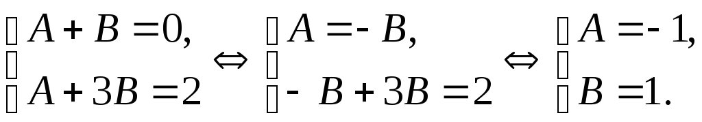
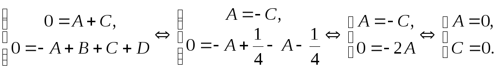
Пусть , – многочлены . Если и , то называют общим делителем многочленов и .
Если общий делитель делится на любой другой общий делитель многочлена, то его называют этих многочленов.
Заметим, что если , то .
Пусть не делит . В таком случае найти один из многочленов можно с помощью алгоритма Евклида. Он основан на многократном применении теоремы о делении с остатком.
Лемма. Если , .
Так же как и в целых числах, линейно выражается через многочлены.
Теперь на ZNZN можно делать свои конспекты
Легко создавать, делиться и просматривать с устройств
Доступно в ПК-версии сайта
