Закон Ома
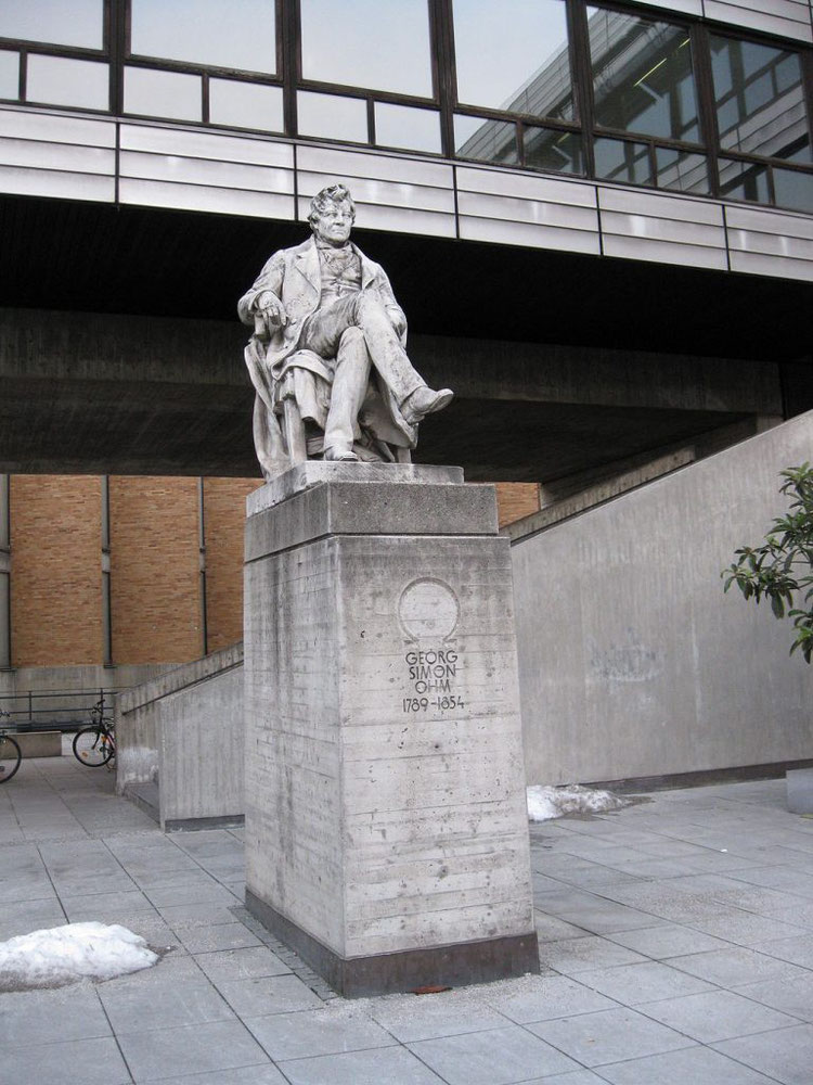
Закон Ома — главный закон электротехники, который открыл в 1826 году выдающийся немецкий ученый Георг Симон Ом. Вместе с экспертом разберем формулировку, формулу и задачи на закон Ома с решением

Физика — наука эмпирическая. Ее основные законы вытекают из практического опыта и частенько много лет не имеют теоретических обоснований. Именно так обстоит дело с главным законом электротехники, который открыл в 1826 году выдающийся немецкий ученый Георг Симон Ом.
Электрические явления люди наблюдали сотни лет. Но никак не связывали между собой заряженность потертого янтаря и молнию. Только на исходе XVIII столетия электричество стали внимательно исследовать. В 1795 году Алессандро Вольта изобрел «вольтов столб», химическую батарею, и обнаружил появление тока в проводнике, соединяющем ее полюса. Сферы применения электричества стремительно множились, и появилась острая необходимость в расчетных формулах для инженеров. Эту задачу решали многие ученые, но первым сформулировал главную формулу электротехники именно Георг Ом. Он ввел в обиход понятие сопротивления и опытным путем установил зависимость между основными характеристиками электрической цепи.
Определение закона Ома простыми словами
Электрическая цепь состоит из двухполюсного источника напряжения, то есть батареи, аккумулятора или генератора. Если полюса источника соединить проводами, то по ним потечет электрический ток. Его величина определяется сопротивлением проводников. Наглядное представление этой зависимости — обыкновенный водопровод. Аналогом источника напряжения является насос или водонапорная башня, создающая давление в магистрали, количество воды, прошедшее по трубе, — подобие силы тока, а кран соответствует сопротивлению. Полностью открытый, он не ограничивает поток, по мере закручивания отверстие для воды уменьшается, пока не закроется совсем.
Закон Ома для участка цепи
Опытным путем исследователь установил взаимосвязь характеристик электрической цепи. Классическая формулировка закона Ома звучит так:
«Сила тока на участке цепи прямо пропорциональна напряжению и обратно пропорциональна сопротивлению».
Формула закона Ома для участка цепи

В таком виде закон Ома приведен в школьных учебниках физики. Согласно этой простой формуле, для определения уровня тока в проводнике достаточно величину напряжения на его сторонах разделить на некий условно постоянный коэффициент, то есть на сопротивление. Почему «условно»? Потому что величина сопротивления может меняться в зависимости от температуры. Поэтому, кстати, лампы накаливания чаще всего перегорают при включении. Сопротивление холодной спирали ниже, чем нагретой, скачок тока при подаче напряжения вызывает ее резкое расширение и разрыв. Но если этот момент преодолен и нить накала уцелела, то ее сопротивление растет, и ток ограничивается. А при температуре жидкого гелия, например, сопротивление падает до нуля, наступает сверхпроводимость.
Закон Ома для замкнутой полной цепи
Предыдущая формулировка годится только для участка цепи, где отсутствует сам источник электродвижущей силы. В реальности ток течет по замкнутому контуру, где обязательно есть батарея или генератор, имеющий собственное внутреннее сопротивление. Поэтому формула закона Ома для полной цепи выглядит несколько сложнее
Формула закона Ома для замкнутой полной цепи

Применение закона Ома
Георг Ом дал в руки инженеров средство для решения задач, связанных с электрическими цепями. Тепловые и световые приборы, электродвигатели, генераторы, линии электропередач, кабели связи рассчитываются на основе этой простой формулы. Нет такой области электротехники, где она не находит применения. Даже в радиотехнике используется закон Ома, но в дифференциальной форме. «Все гениальное — просто», как считали Еврипид, Леонардо да Винчи, Наполеон Бонапарт и Альберт Эйнштейн, несомненные гении. Закон Ома целиком и полностью подтверждает эту истину.
Сила трения
Единицы измерения силы трения, от чего она зависит и какие виды существуют
подробнее

Задача на закон Ома с решением
Задача для участка электрической цепи
Электрочайник, включенный в сеть с напряжением 220 В, потребляет ток 1,1 А. Каково сопротивление электрочайника.
Дано:
U = 220 В
I = 1,1 А
Решение:
Согласно закону Ома для участка цепи:
R=U/I=220/1,1=200 Ом
Ответ: R = 200 Ом.
Задача для полной замкнутой цепи
Источник постоянного тока с ЭДС E = 24 В и внутренним сопротивлением r = 1,5 Ом замкнут на внешнее сопротивление R = 11 Ом. Определить силу тока в цепи.
Дано:
Е=24 В, r=1,5 Ом, R = 11 Ом
Решение:
По закону Ома для замкнутой цепи: I = E/(R + r) = 24/(11+1,5) = 1,92 А.
Ответ: I=1, 92 А.
Популярные вопросы и ответы
Отвечает Николай Герасимов, старший преподаватель физики в Домашней школе «ИнтернетУрок».
Сколько всего законов Ома в физике?
Существует два закона Ома: закон Ома для участка цепи и закон Ома для полной (замкнутой) цепи. Первый связывает сопротивление участка, силу тока в нём и разность потенциалов (напряжение) на его концах. Кроме того, в нем отражено наличие в цепи источника тока.
Второй учитывает и потребителей электрического тока (электрические лампы, обогреватели, телевизоры и так далее), и его источники (генераторы, батарейки, аккумуляторы). Дело в том, что любой источник тока обладает внутренним сопротивление, которое влияет на силу тока. Именно это и учитывается в законе Ома для полной (замкнутой) цепи.
При каких условиях выполняется закон Ома?
Согласно закону Ома, существует линейная зависимость между силой тока в участке цепи и напряжением на его концах. Он отлично выполняется для металлических проводников при любых напряжениях, а вот для тока в вакууме, газе, растворах или расплавах электролитов, полупроводниках линейная зависимость нарушается, и применять закон Ома в том виде, в котором его изучают в школьном курсе, уже нельзя.
Для чего нужен закон Ома?
Трудно переоценить значимость этого закона. Он позволил производить расчет электрических цепей, без которых практически невозможно представить жизнь современного человека, так как они лежат в основе любого электроприбора, начиная от обычной лампы накаливания и заканчивая самыми современными компьютерами.
В каком классе проходят закон Ома?
В школьном курсе ученики впервые знакомятся с электрическими явлениями и законом Ома для участка цепи в 8 классе. Более подробно о причинах возникновения электрического тока и его источниках ученики знакомятся в курсе старшей школы (10 или 11 класс, в зависимости от программы). Здесь же ученики впервые встречаются и с законом Ома для полной (замкнутой) цепи.
Говорят: «не знаешь закон Ома – сиди дома». Так давайте же узнаем (вспомним), что это за закон, и смело пойдем гулять.
Основные понятия закона Ома
Как понять закон Ома? Нужно просто разобраться в том, что есть что в его определении. И начать следует с определения силы тока, напряжения и сопротивления.
Сила тока I
Пусть в каком-то проводнике течет ток. То есть, происходит направленное движение заряженных частиц – допустим, это электроны. Каждый электрон обладает элементарным электрическим зарядом (e= -1,60217662 × 10⁻¹⁹ Кулона). В таком случае через некоторую поверхность за определенный промежуток времени пройдет конкретный электрический заряд, равный сумме всех зарядов протекших электронов.
Отношение заряда к времени и называется силой тока. Чем больший заряд проходит через проводник за определенное время, тем больше сила тока. Сила тока измеряется в Амперах.
Напряжение U, или разность потенциалов
Это как раз та штука, которая заставляет электроны двигаться. Электрический потенциал характеризует способность поля совершать работу по переносу заряда из одной точки в другую. Так, между двумя точками проводника существует разность потенциалов, и электрическое поле совершает работу по переносу заряда.
Физическая величина, равная работе эффективного электрического поля при переносе электрического заряда, и называется напряжением. Измеряется в Вольтах. Один Вольт – это напряжение, которое при перемещении заряда в 1 Кл совершает работу, равную 1 Джоуль.
Сопротивление R
Ток, как известно, течет в проводнике. Пусть это будет какой-нибудь провод. Двигаясь по проводу под действием поля, электроны сталкиваются с атомами провода, проводник греется, атомы в кристаллической решетке начинают колебаться, создавая электронам еще больше проблем для передвижения. Именно это явление и называется сопротивлением. Оно зависит от температуры, материала, сечения проводника и измеряется в Омах.
Формулировка и объяснение закона Ома
Закон немецкого учителя Георга Ома очень прост. Он гласит:
Сила тока на участке цепи прямо пропорционально напряжению и обратно пропорциональна сопротивлению.
Георг Ом вывел этот закон экспериментально (эмпирически) в 1826 году. Естественно, чем больше сопротивление участка цепи, тем меньше будет сила тока. Соответственно, чем больше напряжение, тем и ток будет больше.
Кстати! Для наших читателей сейчас действует скидка 10% на любой вид работы
Данная формулировка закона Ома – самая простая и подходит для участка цепи. Говоря «участок цепи» мы подразумеваем, что это однородный участок, на котором нет источников тока с ЭДС. Говоря проще, этот участок содержит какое-то сопротивление, но на нем нет батарейки, обеспечивающей сам ток.
Если рассматривать закон Ома для полной цепи, формулировка его будет немного иной.
Пусть у нас есть цепь, в ней есть источник тока, создающий напряжение, и какое-то сопротивление.
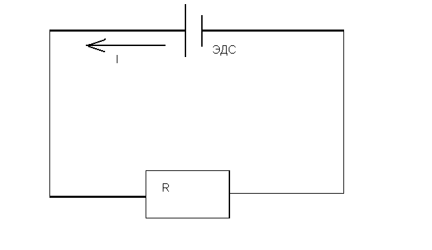
Закон запишется в следующем виде:
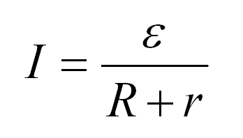
Объяснение закона Ома для полой цепи принципиально не отличается от объяснения для участка цепи. Как видим, сопротивление складывается из собственно сопротивления и внутреннего сопротивления источника тока, а вместо напряжения в формуле фигурирует электродвижущая сила источника.
Кстати, о том, что такое что такое ЭДС, читайте в нашей отдельной статье.
Как понять закон Ома?
Чтобы интуитивно понять закон Ома, обратимся к аналогии представления тока в виде жидкости. Именно так думал Георг Ом, когда проводил опыты, благодаря которым был открыт закон, названный его именем.
Представим, что ток – это не движение частиц-носителей заряда в проводнике, а движение потока воды в трубе. Сначала воду насосом поднимают на водокачку, а оттуда, под действием потенциальной энергии, она стремиться вниз и течет по трубе. Причем, чем выше насос закачает воду, тем быстрее она потечет в трубе.
Отсюда следует вывод, что скорость потока воды (сила тока в проводе) будет тем больше, чем больше потенциальная энергия воды (разность потенциалов)
Сила тока прямо пропорциональна напряжению.
Теперь обратимся к сопротивлению. Гидравлическое сопротивление – это сопротивление трубы, обусловленное ее диаметром и шероховатостью стенок. Логично предположить, что чем больше диаметр, тем меньше сопротивление трубы, и тем большее количество воды (больший ток) протечет через ее сечение.
Сила тока обратно пропорциональна сопротивлению.
Такую аналогию можно проводить лишь для принципиального понимания закона Ома, так как его первозданный вид – на самом деле довольно грубое приближение, которое, тем не менее, находит отличное применение на практике.
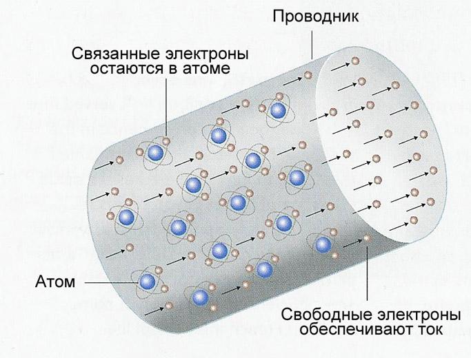
В действительности, сопротивление вещества обусловлено колебанием атомов кристаллической решетки, а ток – движением свободных носителей заряда. В металлах свободными носителями являются электроны, сорвавшиеся с атомных орбит.
В данной статье мы постарались дать простое объяснение закона Ома. Знание этих на первый взгляд простых вещей может сослужить Вам неплохую службу на экзамене. Конечно, мы привели его простейшую формулировку закона Ома и не будем сейчас лезть в дебри высшей физики, разбираясь с активным и реактивным сопротивлениями и прочими тонкостями.
Если у Вас возникнет такая необходимость, Вам с удовольствием помогут сотрудники нашего студенческого сервиса. А напоследок предлагаем Вам посмотреть интересное видео про закон Ома. Это действительно познавательно!
This article is about the law related to electricity. For other uses, see Ohm’s acoustic law.

V, I, and R, the parameters of Ohm’s law
Ohm’s law states that the current through a conductor between two points is directly proportional to the voltage across the two points. Introducing the constant of proportionality, the resistance,[1] one arrives at the usual mathematical equation that describes this relationship:[2]

where I is the current through the conductor, V is the voltage measured across the conductor and R is the resistance of the conductor. More specifically, Ohm’s law states that the R in this relation is constant, independent of the current.[3] If the resistance is not constant, the previous equation cannot be called Ohm’s law, but it can still be used as a definition of static/DC resistance.[4] Ohm’s law is an empirical relation which accurately describes the conductivity of the vast majority of electrically conductive materials over many orders of magnitude of current. However some materials do not obey Ohm’s law; these are called non-ohmic.
The law was named after the German physicist Georg Ohm, who, in a treatise published in 1827, described measurements of applied voltage and current through simple electrical circuits containing various lengths of wire. Ohm explained his experimental results by a slightly more complex equation than the modern form above (see § History below).
In physics, the term Ohm’s law is also used to refer to various generalizations of the law; for example the vector form of the law used in electromagnetics and material science:

where J is the current density at a given location in a resistive material, E is the electric field at that location, and σ (sigma) is a material-dependent parameter called the conductivity. This reformulation of Ohm’s law is due to Gustav Kirchhoff.[5]
History
In January 1781, before Georg Ohm’s work, Henry Cavendish experimented with Leyden jars and glass tubes of varying diameter and length filled with salt solution. He measured the current by noting how strong a shock he felt as he completed the circuit with his body. Cavendish wrote that the «velocity» (current) varied directly as the «degree of electrification» (voltage). He did not communicate his results to other scientists at the time,[6] and his results were unknown until Maxwell published them in 1879.[7]
Francis Ronalds delineated «intensity» (voltage) and «quantity» (current) for the dry pile—a high voltage source—in 1814 using a gold-leaf electrometer. He found for a dry pile that the relationship between the two parameters was not proportional under certain meteorological conditions.[8][9]
Ohm did his work on resistance in the years 1825 and 1826, and published his results in 1827 as the book Die galvanische Kette, mathematisch bearbeitet («The galvanic circuit investigated mathematically»).[10] He drew considerable inspiration from Fourier’s work on heat conduction in the theoretical explanation of his work. For experiments, he initially used voltaic piles, but later used a thermocouple as this provided a more stable voltage source in terms of internal resistance and constant voltage. He used a galvanometer to measure current, and knew that the voltage between the thermocouple terminals was proportional to the junction temperature. He then added test wires of varying length, diameter, and material to complete the circuit. He found that his data could be modeled through the equation

where x was the reading from the galvanometer, ℓ was the length of the test conductor, a depended on the thermocouple junction temperature, and b was a constant of the entire setup. From this, Ohm determined his law of proportionality and published his results.
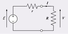
Internal resistance model
In modern notation we would write,

where  is the open-circuit emf of the thermocouple,
  is the internal resistance of the thermocouple and
  is the resistance of the test wire. In terms of the length of the wire this becomes,

where  is the resistance of the test wire per unit length. Thus, Ohm’s coefficients are,

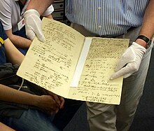
Ohm’s law in Georg Ohm’s lab book.
Ohm’s law was probably the most important of the early quantitative descriptions of the physics of electricity. We consider it almost obvious today. When Ohm first published his work, this was not the case; critics reacted to his treatment of the subject with hostility. They called his work a «web of naked fancies»[11] and the Minister of Education proclaimed that «a professor who preached such heresies was unworthy to teach science.»[12] The prevailing scientific philosophy in Germany at the time asserted that experiments need not be performed to develop an understanding of nature because nature is so well ordered, and that scientific truths may be deduced through reasoning alone.[13] Also, Ohm’s brother Martin, a mathematician, was battling the German educational system. These factors hindered the acceptance of Ohm’s work, and his work did not become widely accepted until the 1840s. However, Ohm received recognition for his contributions to science well before he died.
In the 1850s, Ohm’s law was widely known and considered proved. Alternatives such as «Barlow’s law», were discredited, in terms of real applications to telegraph system design, as discussed by Samuel F. B. Morse in 1855.[14]
The electron was discovered in 1897 by J. J. Thomson, and it was quickly realized that it is the particle (charge carrier) that carries electric currents in electric circuits. In 1900 the first (classical) model of electrical conduction, the Drude model, was proposed by Paul Drude, which finally gave a scientific explanation for Ohm’s law. In this model, a solid conductor consists of a stationary lattice of atoms (ions), with conduction electrons moving randomly in it. A voltage across a conductor causes an electric field, which accelerates the electrons in the direction of the electric field, causing a drift of electrons which is the electric current. However the electrons collide with atoms which causes them to scatter and randomizes their motion, thus converting kinetic energy to heat (thermal energy). Using statistical distributions, it can be shown that the average drift velocity of the electrons, and thus the current, is proportional to the electric field, and thus the voltage, over a wide range of voltages.
The development of quantum mechanics in the 1920s modified this picture somewhat, but in modern theories the average drift velocity of electrons can still be shown to be proportional to the electric field, thus deriving Ohm’s law. In 1927 Arnold Sommerfeld applied the quantum Fermi-Dirac distribution of electron energies to the Drude model, resulting in the free electron model. A year later, Felix Bloch showed that electrons move in waves (Bloch electrons) through a solid crystal lattice, so scattering off the lattice atoms as postulated in the Drude model is not a major process; the electrons scatter off impurity atoms and defects in the material. The final successor, the modern quantum band theory of solids, showed that the electrons in a solid cannot take on any energy as assumed in the Drude model but are restricted to energy bands, with gaps between them of energies that electrons are forbidden to have. The size of the band gap is a characteristic of a particular substance which has a great deal to do with its electrical resistivity, explaining why some substances are electrical conductors, some semiconductors, and some insulators.
While the old term for electrical conductance, the mho (the inverse of the resistance unit ohm), is still used, a new name, the siemens, was adopted in 1971, honoring Ernst Werner von Siemens. The siemens is preferred in formal papers.
In the 1920s, it was discovered that the current through a practical resistor actually has statistical fluctuations, which depend on temperature, even when voltage and resistance are exactly constant; this fluctuation, now known as Johnson–Nyquist noise, is due to the discrete nature of charge. This thermal effect implies that measurements of current and voltage that are taken over sufficiently short periods of time will yield ratios of V/I that fluctuate from the value of R implied by the time average or ensemble average of the measured current; Ohm’s law remains correct for the average current, in the case of ordinary resistive materials.
Ohm’s work long preceded Maxwell’s equations and any understanding of frequency-dependent effects in AC circuits. Modern developments in electromagnetic theory and circuit theory do not contradict Ohm’s law when they are evaluated within the appropriate limits.
Scope
Ohm’s law is an empirical law, a generalization from many experiments that have shown that current is approximately proportional to electric field for most materials. It is less fundamental than Maxwell’s equations and is not always obeyed. Any given material will break down under a strong-enough electric field, and some materials of interest in electrical engineering are «non-ohmic» under weak fields.[15][16]
Ohm’s law has been observed on a wide range of length scales. In the early 20th century, it was thought that Ohm’s law would fail at the atomic scale, but experiments have not borne out this expectation. As of 2012, researchers have demonstrated that Ohm’s law works for silicon wires as small as four atoms wide and one atom high.[17]
Microscopic origins

Drude Model electrons (shown here in blue) constantly bounce among heavier, stationary crystal ions (shown in red).
The dependence of the current density on the applied electric field is essentially quantum mechanical in nature; (see Classical and quantum conductivity.) A qualitative description leading to Ohm’s law can be based upon classical mechanics using the Drude model developed by Paul Drude in 1900.[18][19]
The Drude model treats electrons (or other charge carriers) like pinballs bouncing among the ions that make up the structure of the material. Electrons will be accelerated in the opposite direction to the electric field by the average electric field at their location. With each collision, though, the electron is deflected in a random direction with a velocity that is much larger than the velocity gained by the electric field. The net result is that electrons take a zigzag path due to the collisions, but generally drift in a direction opposing the electric field.
The drift velocity then determines the electric current density and its relationship to E and is independent of the collisions. Drude calculated the average drift velocity from p = −eEτ where p is the average momentum, −e is the charge of the electron and τ is the average time between the collisions. Since both the momentum and the current density are proportional to the drift velocity, the current density becomes proportional to the applied electric field; this leads to Ohm’s law.
Hydraulic analogy
A hydraulic analogy is sometimes used to describe Ohm’s law. Water pressure, measured by pascals (or PSI), is the analog of voltage because establishing a water pressure difference between two points along a (horizontal) pipe causes water to flow. The water volume flow rate, as in liters per second, is the analog of current, as in coulombs per second. Finally, flow restrictors—such as apertures placed in pipes between points where the water pressure is measured—are the analog of resistors. We say that the rate of water flow through an aperture restrictor is proportional to the difference in water pressure across the restrictor. Similarly, the rate of flow of electrical charge, that is, the electric current, through an electrical resistor is proportional to the difference in voltage measured across the resistor. More generally, the hydraulic head may be taken as the analog of voltage, and Ohm’s law is then analogous to Darcy’s law which relates hydraulic head to the volume flow rate via the hydraulic conductivity.
Flow and pressure variables can be calculated in fluid flow network with the use of the hydraulic ohm analogy.[20][21] The method can be applied to both steady and transient flow situations. In the linear laminar flow region, Poiseuille’s law describes the hydraulic resistance of a pipe, but in the turbulent flow region the pressure–flow relations become nonlinear.
The hydraulic analogy to Ohm’s law has been used, for example, to approximate blood flow through the circulatory system.[22]
Circuit analysis
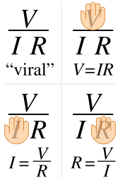
Covering the unknown in the Ohm’s law image mnemonic gives the formula in terms of the remaining parameters
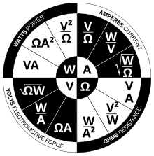
Ohm’s law wheel with international unit symbols
In circuit analysis, three equivalent expressions of Ohm’s law are used interchangeably:

Each equation is quoted by some sources as the defining relationship of Ohm’s law,[2][23][24]
or all three are quoted,[25] or derived from a proportional form,[26]
or even just the two that do not correspond to Ohm’s original statement may sometimes be given.[27][28]
The interchangeability of the equation may be represented by a triangle, where V (voltage) is placed on the top section, the I (current) is placed to the left section, and the R (resistance) is placed to the right. The divider between the top and bottom sections indicates division (hence the division bar).
Resistive circuits
Resistors are circuit elements that impede the passage of electric charge in agreement with Ohm’s law, and are designed to have a specific resistance value R. In schematic diagrams, a resistor is shown as a long rectangle or zig-zag symbol. An element (resistor or conductor) that behaves according to Ohm’s law over some operating range is referred to as an ohmic device (or an ohmic resistor) because Ohm’s law and a single value for the resistance suffice to describe the behavior of the device over that range.
Ohm’s law holds for circuits containing only resistive elements (no capacitances or inductances) for all forms of driving voltage or current, regardless of whether the driving voltage or current is constant (DC) or time-varying such as AC. At any instant of time Ohm’s law is valid for such circuits.
Resistors which are in series or in parallel may be grouped together into a single «equivalent resistance» in order to apply Ohm’s law in analyzing the circuit.
Reactive circuits with time-varying signals
When reactive elements such as capacitors, inductors, or transmission lines are involved in a circuit to which AC or time-varying voltage or current is applied, the relationship between voltage and current becomes the solution to a differential equation, so Ohm’s law (as defined above) does not directly apply since that form contains only resistances having value R, not complex impedances which may contain capacitance (C) or inductance (L).
Equations for time-invariant AC circuits take the same form as Ohm’s law. However, the variables are generalized to complex numbers and the current and voltage waveforms are complex exponentials.[29]
In this approach, a voltage or current waveform takes the form Aest, where t is time, s is a complex parameter, and A is a complex scalar. In any linear time-invariant system, all of the currents and voltages can be expressed with the same s parameter as the input to the system, allowing the time-varying complex exponential term to be canceled out and the system described algebraically in terms of the complex scalars in the current and voltage waveforms.
The complex generalization of resistance is impedance, usually denoted Z; it can be shown that for an inductor,

and for a capacitor,

We can now write,

where V and I are the complex scalars in the voltage and current respectively and Z is the complex impedance.
This form of Ohm’s law, with Z taking the place of R, generalizes the simpler form. When Z is complex, only the real part is responsible for dissipating heat.
In a general AC circuit, Z varies strongly with the frequency parameter s, and so also will the relationship between voltage and current.
For the common case of a steady sinusoid, the s parameter is taken to be  , corresponding to a complex sinusoid
  . The real parts of such complex current and voltage waveforms describe the actual sinusoidal currents and voltages in a circuit, which can be in different phases due to the different complex scalars.
Linear approximations
Ohm’s law is one of the basic equations used in the analysis of electrical circuits. It applies to both metal conductors and circuit components (resistors) specifically made for this behaviour. Both are ubiquitous in electrical engineering. Materials and components that obey Ohm’s law are described as «ohmic»[30] which means they produce the same value for resistance (R = V/I) regardless of the value of V or I which is applied and whether the applied voltage or current is DC (direct current) of either positive or negative polarity or AC (alternating current).
In a true ohmic device, the same value of resistance will be calculated from R = V/I regardless of the value of the applied voltage V. That is, the ratio of V/I is constant, and when current is plotted as a function of voltage the curve is linear (a straight line). If voltage is forced to some value V, then that voltage V divided by measured current I will equal R. Or if the current is forced to some value I, then the measured voltage V divided by that current I is also R. Since the plot of I versus V is a straight line, then it is also true that for any set of two different voltages V1 and V2 applied across a given device of resistance R, producing currents I1 = V1/R and I2 = V2/R, that the ratio (V1 − V2)/(I1 − I2) is also a constant equal to R. The operator «delta» (Δ) is used to represent a difference in a quantity, so we can write ΔV = V1 − V2 and ΔI = I1 − I2. Summarizing, for any truly ohmic device having resistance R, V/I = ΔV/ΔI = R for any applied voltage or current or for the difference between any set of applied voltages or currents.
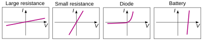
The I–V curves of four devices: Two resistors, a diode, and a battery. The two resistors follow Ohm’s law: The plot is a straight line through the origin. The other two devices do not follow Ohm’s law.
There are, however, components of electrical circuits which do not obey Ohm’s law; that is, their relationship between current and voltage (their I–V curve) is nonlinear (or non-ohmic). An example is the p–n junction diode (curve at right). As seen in the figure, the current does not increase linearly with applied voltage for a diode. One can determine a value of current (I) for a given value of applied voltage (V) from the curve, but not from Ohm’s law, since the value of «resistance» is not constant as a function of applied voltage. Further, the current only increases significantly if the applied voltage is positive, not negative. The ratio V/I for some point along the nonlinear curve is sometimes called the static, or chordal, or DC, resistance,[31][32] but as seen in the figure the value of total V over total I varies depending on the particular point along the nonlinear curve which is chosen. This means the «DC resistance» V/I at some point on the curve is not the same as what would be determined by applying an AC signal having peak amplitude ΔV volts or ΔI amps centered at that same point along the curve and measuring ΔV/ΔI. However, in some diode applications, the AC signal applied to the device is small and it is possible to analyze the circuit in terms of the dynamic, small-signal, or incremental resistance, defined as the one over the slope of the V–I curve at the average value (DC operating point) of the voltage (that is, one over the derivative of current with respect to voltage). For sufficiently small signals, the dynamic resistance allows the Ohm’s law small signal resistance to be calculated as approximately one over the slope of a line drawn tangentially to the V–I curve at the DC operating point.[33]
Temperature effects
Ohm’s law has sometimes been stated as, «for a conductor in a given state, the electromotive force is proportional to the current produced.» That is, that the resistance, the ratio of the applied electromotive force (or voltage) to the current, «does not vary with the current strength .» The qualifier «in a given state» is usually interpreted as meaning «at a constant temperature,» since the resistivity of materials is usually temperature dependent. Because the conduction of current is related to Joule heating of the conducting body, according to Joule’s first law, the temperature of a conducting body may change when it carries a current. The dependence of resistance on temperature therefore makes resistance depend upon the current in a typical experimental setup, making the law in this form difficult to directly verify. Maxwell and others worked out several methods to test the law experimentally in 1876, controlling for heating effects.[34]
Relation to heat conductions
Ohm’s principle predicts the flow of electrical charge (i.e. current) in electrical conductors when subjected to the influence of voltage differences; Jean-Baptiste-Joseph Fourier’s principle predicts the flow of heat in heat conductors when subjected to the influence of temperature differences.
The same equation describes both phenomena, the equation’s variables taking on different meanings in the two cases. Specifically, solving a heat conduction (Fourier) problem with temperature (the driving «force») and flux of heat (the rate of flow of the driven «quantity», i.e. heat energy) variables also solves an analogous electrical conduction (Ohm) problem having electric potential (the driving «force») and electric current (the rate of flow of the driven «quantity», i.e. charge) variables.
The basis of Fourier’s work was his clear conception and definition of thermal conductivity. He assumed that, all else being the same, the flux of heat is strictly proportional to the gradient of temperature. Although undoubtedly true for small temperature gradients, strictly proportional behavior will be lost when real materials (e.g. ones having a thermal conductivity that is a function of temperature) are subjected to large temperature gradients.
A similar assumption is made in the statement of Ohm’s law: other things being alike, the strength of the current at each point is proportional to the gradient of electric potential. The accuracy of the assumption that flow is proportional to the gradient is more readily tested, using modern measurement methods, for the electrical case than for the heat case.
Other versions
Ohm’s law, in the form above, is an extremely useful equation in the field of electrical/electronic engineering because it describes how voltage, current and resistance are interrelated on a «macroscopic» level, that is, commonly, as circuit elements in an electrical circuit. Physicists who study the electrical properties of matter at the microscopic level use a closely related and more general vector equation, sometimes also referred to as Ohm’s law, having variables that are closely related to the V, I, and R scalar variables of Ohm’s law, but which are each functions of position within the conductor. Physicists often use this continuum form of Ohm’s Law:[35]

where «E» is the electric field vector with units of volts per meter (analogous to «V» of Ohm’s law which has units of volts), «J» is the current density vector with units of amperes per unit area (analogous to «I» of Ohm’s law which has units of amperes), and «ρ» (Greek «rho») is the resistivity with units of ohm·meters (analogous to «R» of Ohm’s law which has units of ohms). The above equation is sometimes written[36] as J = σE where «σ» (Greek «sigma») is the conductivity which is the reciprocal of ρ.

Current flowing through a uniform cylindrical conductor (such as a round wire) with a uniform field applied.
The voltage between two points is defined as:[37]

with  the element of path along the integration of electric field vector E. If the applied E field is uniform and oriented along the length of the conductor as shown in the figure, then defining the voltage V in the usual convention of being opposite in direction to the field (see figure), and with the understanding that the voltage V is measured differentially across the length of the conductor allowing us to drop the Δ symbol, the above vector equation reduces to the scalar equation:

Since the E field is uniform in the direction of wire length, for a conductor having uniformly consistent resistivity ρ, the current density J will also be uniform in any cross-sectional area and oriented in the direction of wire length, so we may write:[38]

Substituting the above 2 results (for E and J respectively) into the continuum form shown at the beginning of this section:

The electrical resistance of a uniform conductor is given in terms of resistivity by:[38]

where ℓ is the length of the conductor in SI units of meters, a is the cross-sectional area (for a round wire a = πr2 if r is radius) in units of meters squared, and ρ is the resistivity in units of ohm·meters.
After substitution of R from the above equation into the equation preceding it, the continuum form of Ohm’s law for a uniform field (and uniform current density) oriented along the length of the conductor reduces to the more familiar form:

A perfect crystal lattice, with low enough thermal motion and no deviations from periodic structure, would have no resistivity,[39] but a real metal has crystallographic defects, impurities, multiple isotopes, and thermal motion of the atoms. Electrons scatter from all of these, resulting in resistance to their flow.
The more complex generalized forms of Ohm’s law are important to condensed matter physics, which studies the properties of matter and, in particular, its electronic structure. In broad terms, they fall under the topic of constitutive equations and the theory of transport coefficients.
Magnetic effects
If an external B-field is present and the conductor is not at rest but moving at velocity v, then an extra term must be added to account for the current induced by the Lorentz force on the charge carriers.

In the rest frame of the moving conductor this term drops out because v = 0. There is no contradiction because the electric field in the rest frame differs from the E-field in the lab frame: E′ = E + v × B.
Electric and magnetic fields are relative, see Lorentz transformation.
If the current J is alternating because the applied voltage or E-field varies in time, then reactance must be added to resistance to account for self-inductance, see electrical impedance. The reactance may be strong if the frequency is high or the conductor is coiled.
Conductive fluids
In a conductive fluid, such as a plasma, there is a similar effect. Consider a fluid moving with the velocity  in a magnetic field
  . The relative motion induces an electric field
  which exerts electric force on the charged particles giving rise to an electric current
  . The equation of motion for the electron gas, with a number density
  , is written as

where  ,
,  and
and  are the charge, mass and velocity of the electrons, respectively. Also,
  is the frequency of collisions of the electrons with ions which have a velocity field
  . Since, the electron has a very small mass compared with that of ions, we can ignore the left hand side of the above equation to write

where we have used the definition of the current density, and also put  which is the electrical conductivity. This equation can also be equivalently written as

where  is the electrical resistivity. It is also common to write
  instead of
  which can be confusing since it is the same notation used for the magnetic diffusivity defined as
  .
.
See also
- Fick’s law of diffusion
- Hopkinson’s law («Ohm’s law for magnetics»)
- Maximum power transfer theorem
- Norton’s theorem
- Sheet resistance
- Superposition theorem
- Thermal noise
- Thévenin’s theorem
References
- ^ Consoliver, Earl L. & Mitchell, Grover I. (1920). Automotive Ignition Systems. McGraw-Hill. p. 4.
- ^ a b Millikan, Robert A.; Bishop, E. S. (1917). Elements of Electricity. American Technical Society. p. 54.
- ^
Heaviside, Oliver (1894). Electrical Papers. Vol. 1. Macmillan and Co. p. 283. ISBN 978-0-8218-2840-3. - ^
Young, Hugh; Freedman, Roger (2008). Sears and Zemansky’s University Physics: With Modern Physics. Vol. 2 (12 ed.). Pearson. p. 853. ISBN 978-0-321-50121-9. - ^ Darrigol, Olivier (8 June 2000). Electrodynamics from Ampère to Einstein. p. 70. ISBN 9780198505945..
- ^ Fleming, John Ambrose (1911). «Electricity» . In Chisholm, Hugh (ed.). Encyclopædia Britannica. Vol. 9 (11th ed.). Cambridge University Press. p. 182.
- ^ Bordeau, Sanford P. (1982). Volts to Hertz— the Rise of Electricity: From the Compass to the Radio Through the Works of Sixteen Great Men of Science Whose Names are Used in Measuring Electricity and Magnetism. pp. 86–107. ISBN 9780808749080.
- ^ Ronalds, B. F. (2016). Sir Francis Ronalds: Father of the Electric Telegraph. London: Imperial College Press. ISBN 978-1-78326-917-4.
- ^ Ronalds, B. F. (July 2016). «Francis Ronalds (1788–1873): The First Electrical Engineer?». Proceedings of the IEEE. 104 (7): 1489–1498. doi:10.1109/JPROC.2016.2571358. S2CID 20662894.
- ^ Ohm, G. S. (1827). Die galvanische Kette, mathematisch bearbeitet (PDF). Berlin: T. H. Riemann. Archived from the original (PDF) on 2009-03-26.
- ^ Davies, Brian (1980). «A web of naked fancies?». Physics Education. 15 (1): 57–61. Bibcode:1980PhyEd..15…57D. doi:10.1088/0031-9120/15/1/314. S2CID 250832899.
- ^ Hart, Ivor Blashka (1923). Makers of Science. London: Oxford University Press. p. 243. OL 6662681M..
- ^ Schnädelbach, Herbert (14 June 1984). Philosophy in Germany 1831-1933. pp. 78–79. ISBN 9780521296465.
- ^ Taliaferro Preston (1855). Shaffner’s Telegraph Companion: Devoted to the Science and Art of the Morse Telegraph. Vol. 2. Pudney & Russell.
- ^ Purcell, Edward M. (1985), Electricity and magnetism, Berkeley Physics Course, vol. 2 (2nd ed.), McGraw-Hill, p. 129, ISBN 978-0-07-004908-6
- ^ Griffiths, David J. (1999), Introduction to electrodynamics (3rd ed.), Prentice Hall, p. 289, ISBN 978-0-13-805326-0
- ^ Weber, B.; Mahapatra, S.; Ryu, H.; Lee, S.; Fuhrer, A.; Reusch, T. C. G.; Thompson, D. L.; Lee, W. C. T.; Klimeck, G.; Hollenberg, L. C. L.; Simmons, M. Y. (2012). «Ohm’s Law Survives to the Atomic Scale». Science. 335 (6064): 64–67. Bibcode:2012Sci…335…64W. doi:10.1126/science.1214319. PMID 22223802. S2CID 10873901.
- ^ Drude, Paul (1900). «Zur Elektronentheorie der Metalle». Annalen der Physik. 306 (3): 566–613. Bibcode:1900AnP…306..566D. doi:10.1002/andp.19003060312.[dead link]
- ^ Drude, Paul (1900). «Zur Elektronentheorie der Metalle; II. Teil. Galvanomagnetische und thermomagnetische Effecte». Annalen der Physik. 308 (11): 369–402. Bibcode:1900AnP…308..369D. doi:10.1002/andp.19003081102.[dead link]
- ^ A. Akers; M. Gassman & R. Smith (2006). Hydraulic Power System Analysis. New York: Taylor & Francis. Chapter 13. ISBN 978-0-8247-9956-4.
- ^ A. Esposito, «A Simplified Method for Analyzing Circuits by Analogy», Machine Design, October 1969, pp. 173–177.
- ^ Guyton, Arthur; Hall, John (2006). «Chapter 14: Overview of the Circulation; Medical Physics of Pressure, Flow, and Resistance». In Gruliow, Rebecca (ed.). Textbook of Medical Physiology (11th ed.). Philadelphia, Pennsylvania: Elsevier Inc. p. 164. ISBN 978-0-7216-0240-0.
- ^ Nilsson, James William & Riedel, Susan A. (2008). Electric circuits. Prentice Hall. p. 29. ISBN 978-0-13-198925-2.
- ^ Halpern, Alvin M. & Erlbach, Erich (1998). Schaum’s outline of theory and problems of beginning physics II. McGraw-Hill Professional. p. 140. ISBN 978-0-07-025707-8.
- ^ Patrick, Dale R. & Fardo, Stephen W. (1999). Understanding DC circuits. Newnes. p. 96. ISBN 978-0-7506-7110-1.
- ^ O’Conor Sloane, Thomas (1909). Elementary electrical calculations. D. Van Nostrand Co. p. 41.
R= Ohm’s law proportional.
- ^ Cumming, Linnaeus (1902). Electricity treated experimentally for the use of schools and students. Longman’s Green and Co. p. 220.
V=IR Ohm’s law.
- ^ Stein, Benjamin (1997). Building technology (2nd ed.). John Wiley and Sons. p. 169. ISBN 978-0-471-59319-5.
- ^ Prasad, Rajendra (2006). Fundamentals of Electrical Engineering. Prentice-Hall of India. ISBN 978-81-203-2729-0.
- ^ Hughes, E, Electrical Technology, pp10, Longmans, 1969.
- ^ Brown, Forbes T. (2006). Engineering System Dynamics. CRC Press. p. 43. ISBN 978-0-8493-9648-9.
- ^ Kaiser, Kenneth L. (2004). Electromagnetic Compatibility Handbook. CRC Press. pp. 13–52. ISBN 978-0-8493-2087-3.
- ^ Horowitz, Paul; Hill, Winfield (1989). The Art of Electronics (2nd ed.). Cambridge University Press. p. 13. ISBN 978-0-521-37095-0.
- ^
Normal Lockyer, ed. (September 21, 1876). «Reports». Nature. Macmillan Journals Ltd. 14 (360): 451–459 [452]. Bibcode:1876Natur..14..451.. doi:10.1038/014451a0. - ^ Lerner, Lawrence S. (1977). Physics for scientists and engineers. Jones & Bartlett. p. 736. ISBN 978-0-7637-0460-5.
- ^ Seymour J, Physical Electronics, Pitman, 1972, pp. 53–54
- ^ Lerner L, Physics for scientists and engineers, Jones & Bartlett, 1997, pp. 685–686
- ^ a b Lerner L, Physics for scientists and engineers, Jones & Bartlett, 1997, pp. 732–733
- ^ Seymour J, Physical Electronics, pp. 48–49, Pitman, 1972
External links and further reading
![]()
Wikimedia Commons has media related to Ohm’s law.
- Ohm’s Law chapter from Lessons In Electric Circuits Vol 1 DC book and series.
- John C. Shedd and Mayo D. Hershey,»The History of Ohm’s Law», Popular Science, December 1913, pp. 599–614, Bonnier Corporation ISSN 0161-7370, gives the history of Ohm’s investigations, prior work, Ohm’s false equation in the first paper, illustration of Ohm’s experimental apparatus.
- Schagrin, Morton L. (1963). «Resistance to Ohm’s Law». American Journal of Physics. 31 (7): 536–547. Bibcode:1963AmJPh..31..536S. doi:10.1119/1.1969620. S2CID 120421759. Explores the conceptual change underlying Ohm’s experimental work.
- Kenneth L. Caneva, «Ohm, Georg Simon.» Complete Dictionary of Scientific Biography. 2008
- s:Scientific Memoirs/2/The Galvanic Circuit investigated Mathematically, a translation of Ohm’s original paper.

{I = dfrac{U}{R}}
На этой странице вы можете рассчитать силу тока, напряжение и сопротивление по закону Ома для участка цепи с помощью удобного калькулятора онлайн
Закон Ома — один из фундаментальных законов электродинамики, который определяет взаимосвязь между напряжением, сопротивлением и силой тока. Он был открыт эмпирическим путем Георгом Омом в 1826 году.
Содержание:
- калькулятор закона Ома
- закон Ома для участка цепи
- формула силы тока
- формула напряжения
- формула сопротивления
- примеры задач
Закон Ома для участка цепи
Сила тока прямо пропорциональна напряжению и обратно пропорциональна сопротивлению участка цепи I= dfrac{U}{R}
Формула силы тока
Формула позволяет найти силу тока I через напряжение U и сопротивление R по закону Ома для участка цепи.

{I = dfrac{U}{R}}
I — сила тока
U — напряжение
R — сопротивление
Сила тока (I) в проводнике прямо пропорциональна напряжению (U) на его концах и обратно пропорциональна его сопротивлению (R).
Формула напряжения
Формула позволяет найти напряжение U через силу тока I и сопротивление R по закону Ома для участка цепи.
{U = I cdot R}
U — напряжение
I — сила тока
R — сопротивление
Падение напряжение на проводнике равно произведению сопротивления проводника на силу тока в нем.
Формула сопротивления
Формула позволяет найти сопротивление R через силу тока I и напряжение U по закону Ома для участка цепи.
{R = dfrac{U}{I}}
R — сопротивление
U — напряжение
I — сила тока
Сопротивление проводника прямо пропорционально напряжению на его концах и обратно пропорционально величине силы тока, протекающего через него.
Примеры задач на нахождение силы тока, напряжения и сопротивления по закону Ома
Задача 1
Найдите силу тока в участке цепи, если его сопротивление 40 Ом, а напряжение на его концах 4 В.
Решение
Воспользуемся формулой силы тока. Подставим в нее значения напряжения и сопротивления, после чего останется произвести простейший математический расчет.
I = dfrac{U}{R} = dfrac{4}{40} = 0.1 А
Ответ: 0.1 А
На этой странице есть калькулятор, который поможет проверить полученный ответ.
Задача 2
Найдите напряжение на концах нагревательного элемента, если его сопротивление 40 Ом, а сила тока 2А.
Решение
Для решения этой задачи нам пригодится формула напряжения.
U = I cdot R = 2 cdot 40 = 80 В
Ответ: 80 В
Проверим получившийся результат с помощью калькулятора .
Задача 3
Найдите сопротивление спирали, сила тока в которой 0.5 А, а напряжение на ее концах 120 В.
Решение
Чтобы найти сопротивление спирали нам потребуется формула сопротивления.
R = dfrac{U}{I} = dfrac{120}{0.5} = 240 Ом
Ответ: 240 Ом
Проверка .
Урок физики в 9-м классе по теме:
‘Закон Ома’.
Цель урока: знакомство с законом Ома и применение его при решении задач. Развитие межпредметных связей между математикой и физикой.
Оборудование: вольтметр, амперметр, резистор, реостат, источник питания, соединительные провода.
План урока.
1. организационный момент. (подготовка класса к уроку).
2. проверка домашнего задания. Рассказать про резисторы.
3. выступление математика по темам: прямая пропорциональность, график, обратная пропорциональность, график.
Как нам уже давно известно, математика зародилась тысячи лет назад и создавалась для решения многочисленных практических задач, возникавших и в жизни каждого человека, и в жизни человеческих сообществ. Особый интерес для практики представляют формулы, то есть верные равенства, описывающие зависимости между величинами.
Зависимость между величинами бывают разные: 1) если две величины изменяются таким образом, что отношение соответствующих значений этих величин остается числом постоянным, то такие величины называются прямо пропорциональными. Пример: зависимость расстояния и времени равномерного движения является прямой пропорциональностью: s = υ*t.
Прямо пропорциональные величины можно охарактеризовать еще и так: с увеличением ( уменьшением) одной величины в несколько раз другая величина увеличивается ( уменьшается) во столько же раз.
2). Если две величины изменяются так, что произведение соответствующих значений этих величин остается числом постоянным, то такие величины называются обратно пропорциональными. Обратно пропорциональные величины можно охарактеризовать так: с увеличением ( уменьшением) одной величины в несколько раз другая величина уменьшается ( увеличивается) во столько же раз.
Мы с вами знаем график зависимости прямой пропорциональности y = x, обратной пропорциональности y=1/x. Давайте повторим их и поработаем по графикам.
Два ученика строят графики функций: y=6/x; y=12/x; y=24/x; y=36/x — первый.
y=x; y=2x; y=4x; y=5x- второй.
Остальные работают с учителем по карточкам:
Постройте формулу, описывающую зависимости между величинами. Какая это зависимость?
1) Лыжник идет со скоростью 6 км/ч какое расстояние он пройдет за 2,5 ч? за какое время он пройдет 27 км?
2) Килограмм картошки стоит 6 руб. Сколько надо заплатить за 2,5 кг картошки? Сколько картошки можно купить на 27 руб?
3) Через кран поступает в минуту 6 л воды. Сколько воды поступит через кран за 2,5 мин? За сколько времени через кран поступит 27 л воды?
4) Минутная стрелка поворачивается за 1 мин на угол 6°. На какой угол повернется она за 2,5 мин? За сколько времени повернется минутная стрелка на угол 27°?
На чертежах представлены графики( графики построенные двумя учениками). Определите по ним коэффициенты пропорциональности и их формулы. Как зависит расположение графика функции от коэффициента пропорциональности? Теперь полученные знания применим на уроке физики.
Работа класса с учителем физики.
4. вольт-амперная характеристика проводника.
a) Опыт выясняющий зависимость силы тока от напряжения при постоянном сопротивлении: I~U
U I U
2U 2I
3U 3I
I
b) Опыт выясняющий зависимость силы тока от сопротивления при постоянном напряжении: I~1/R I
R I
2R I/2
3R I/3
R
5. Закон Ома. I~U; I~1/R I=U/R.
Сила тока в участке цепи прямо пропорционально напряжению на этом участке и обратно пропорциональна его сопротивлению.
5. короткое замыкание — соединение 2 точек электрической цепи, находящимся под напряжением, коротким проводником, обладающим очень малым сопротивлением.
6. решение задач . на рисунке изображены графики 1,2 зависимости I от U для 2 проводников. Какой из этих проводников обладает большим сопротивлением?
I,А
1
2
U,В
7. домашнее задание 12 ?45,47,50.
8. закрепление 1. как изменится сила тока на участке цепи, если при неизменном сопротивлении увеличить напряжение на его концах?
2. как изменится сила тока на участке цепи, если при неизменном напряжении увеличить сопротивление участка цепи?
3. по какой формуле находится напряжение, если известны сила тока и сопротивление данного участка.
4. что называют коротким замыканием? Почему при этом увеличивается сила тока?