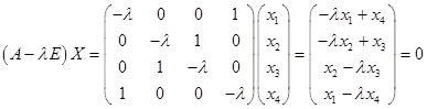
1) Составить характеристическое уравнение линейного оператора |A — l.E| = 0.
2) Найдем все корни характеристического уравнения.
3) Вычислим собственные векторы линейного оператора A, решая матричное уравнение (A — l.E)X=0.
4) Ортонормируем, полученный базис.
Пример. Линейный оператор A, действующий в евклидовом пространстве Е3, имеет в ортонормированном базисе E1, E2, E3 матрицу
 .
.
Найти в Е3 ортонормированный базис из собственных векторов оператора A и составить матрицу оператора A в этом базисе.
Решение. 1) Составить характеристическое уравнение линейного оператора |A — l.E| = 0.

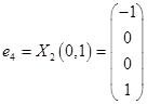
2) Найдем все корни характеристического уравнения: l1=-1, l2 = l3 = 1. Тогда матрица линейного оператора в ортонормированном базисе, составленном из собственных векторов имеет вид
![]() .
.
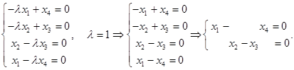
3) Вычислим собственные векторы линейного оператора A, решая матричное уравнение (A — l.E)X=0.
Пусть l1=-1. Матричное уравнение (A — l1E)X=0 принимает вид:

Решая систему, находим решение X = C(1,-2,1), C€R.
Пусть l2 = l3 = 1. Матричное уравнение (A — l1E)X=0 принимает вид:

Решая систему, находим решение X = C1(2,1,0) + C2(-1,0,1), C€R.
4) Ортонормируем, полученный базис.
A1 = (1,-2,1), A2 = (2,1,0), A3 =(-1,0,1).
B1 = (1,-2,1), B2 = (2,1,0), B3 = A3 + k b2, ![]() , b3 =(-1/5, 2/5, 1/5).
, b3 =(-1/5, 2/5, 1/5).
 .
.
| < Предыдущая | Следующая > |
|---|
104. Построение ортонормированного базиса из собственных векторов самосопряженного оператора
1) Составить характеристическое уравнение линейного оператора |A — l.E| = 0.
2) Найдем все корни характеристического уравнения.
3) Вычислим собственные векторы линейного оператора A, решая матричное уравнение (A — l.E)X=0.
4) Ортонормируем, полученный базис.
Пример. Линейный оператор A, действующий в евклидовом пространстве Е3, имеет в ортонормированном базисе E1, E2, E3 матрицу
.
Найти в Е3 ортонормированный базис из собственных векторов оператора A и составить матрицу оператора A в этом базисе.
Решение. 1) Составить характеристическое уравнение линейного оператора |A — l.E| = 0.
2) Найдем все корни характеристического уравнения: l1=-1, l2 = l3 = 1. Тогда матрица линейного оператора в ортонормированном базисе, составленном из собственных векторов имеет вид
 .
.
3) Вычислим собственные векторы линейного оператора A, решая матричное уравнение (A — l.E)X=0.
Пусть l1=-1. Матричное уравнение (A — l1E)X=0 принимает вид:
Пусть l2 = l3 = 1. Матричное уравнение (A — l1E)X=0 принимает вид:
4) Ортонормируем, полученный базис.
B1 = (1,-2,1), B2 = (2,1,0), B3 = A3 + k b2,  , b3 =(-1/5, 2/5, 1/5).
.
Собственные числа и собственные векторы линейного оператора
Определение . Ненулевой вектор x называется собственным вектором оператора A , если оператор A переводит x в коллинеарный ему вектор, то есть A· x = λ· x . Число λ называется собственным значением или собственным числом оператора A, соответствующим собственному вектору x .
Отметим некоторые свойства собственных чисел и собственных векторов.
1. Любая линейная комбинация собственных векторов x 1, x 2, . x m оператора A , отвечающих одному и тому же собственному числу λ, является собственным вектором с тем же собственным числом.
2. Собственные векторы x 1, x 2, . x m оператора A с попарно различными собственными числами λ1, λ2, …, λm линейно независимы.
3. Если собственные числа λ1=λ2= λm= λ, то собственному числу λ соответствует не более m линейно независимых собственных векторов.
Итак, если имеется n линейно независимых собственных векторов x 1, x 2, . x n, соответствующих различным собственным числам λ1, λ2, …, λn, то они линейно независимы, следовательно, их можно принять за базис пространства Rn. Найдем вид матрицы линейного оператора A в базисе из его собственных векторов, для чего подействуем оператором A на базисные векторы:  тогда
тогда  .
.
Таким образом, матрица линейного оператора A в базисе из его собственных векторов имеет диагональный вид, причем по диагонали стоят собственные числа оператора A.
Существует ли другой базис, в котором матрица имеет диагональный вид? Ответ на поставленный вопрос дает следующая теорема.
Теорема. Матрица линейного оператора A в базисе < ε i> (i = 1..n) имеет диагональный вид тогда и только тогда, когда все векторы базиса — собственные векторы оператора A.
Правило отыскания собственных чисел и собственных векторов
Система (1) имеет ненулевое решение, если ее определитель D равен нулю
Пример №1 . Линейный оператор A действует в R3 по закону A· x =(x1-3x2+4x3, 4x1-7x2+8x3, 6x1-7x2+7x3), где x1, x2, . xn — координаты вектора x в базисе e 1=(1,0,0), e 2=(0,1,0), e 3=(0,0,1). Найти собственные числа и собственные векторы этого оператора.
Решение. Строим матрицу этого оператора:
A· e 1=(1,4,6)
A· e 2=(-3,-7,-7)
A· e 3=(4,8,7)  .
.
Составляем систему для определения координат собственных векторов:
(1-λ)x1-3x2+4x3=0
x1-(7+λ)x2+8x3=0
x1-7x2+(7-λ)x3=0
Составляем характеристическое уравнение и решаем его:
Пример №2 . Дана матрица  .
.
1. Доказать, что вектор x =(1,8,-1) является собственным вектором матрицы A. Найти собственное число, соответствующее этому собственному вектору.
2. Найти базис, в котором матрица A имеет диагональный вид.
Решение находим с помощью калькулятора.
1. Если A· x =λ· x , то x — собственный вектор
Определение . Симметрической матрицей называется квадратная матрица, в которой элементы, симметричные относительно главной диагонали, равны, то есть в которой ai k =ak i .
Замечания .
- Все собственные числа симметрической матрицы вещественны.
- Собственные векторы симметрической матрицы, соответствующие попарно различным собственным числам, ортогональны.
В качестве одного из многочисленных приложений изученного аппарата, рассмотрим задачу об определении вида кривой второго порядка.
http://math.semestr.ru/math/vector.php
![]()
Построение ортонормированного базиса из собственных
векторов для симметричного линейного оператора
На прошлой лекции мы изучили ортогональные и симметричные операторы в евклидовом пространстве.
Мы выяснили, что
Ортогональная матрица может не иметь действительных собственных значений.
Симметрическая матрица ВСЕГДА имеет действительное собственное значение.
Все собственные значения симметрической матрицы – действительные числа.
Собственные векторы симметрической матрицы, принадлежащие различным собственным значениям, ортогональны.
Для любой симметрической вещественной матрицы A существует ортогональная матрица U, такая, что матрица U-1AU – диагональная матрица.
Алгоритм нахождения ортонормированного базиса из собственных векторов симметрической матрицы:
I. Найти характеристические числа i заданной симметрической матрицы.
II. Если i — простой корень характеристического уравнения, то ему отвечает с точностью до множителя один собственный вектор. Нормируем его и получаем единичный вектор.
Если i — корень кратности k , то ему отвечают k линейно независимых собственных векторов. В этом случае их необходимо отогонализировать и подвергнуть нормировке — получаем k линейно независимых ортонормированных вектора,
отвечающих собственному значению i . Так как собственные векторы, отвечающие различным характеристическим числам, ортогональны, то, собирая их вместе,
получаем ортонормированный базис из собственных векторов.

Пример 1. Привести к диагональному виду с помощью ортогональной матрицы
|
1 |
2 |
2 |
|||
|
симметрическую матрицу A |
2 |
1 |
2 |
. Указать ортонормированный базис. |
|
|
2 |
2 |
1 |
|||
Решение.
На первом шаге необходимо найти собственные значения данного линейного оператора.
Составим характеристическое уравнение данного преобразования: Ae E 0 .
|
2 |
2 |
II III |
5 |
5 |
5 |
|||||||||||
|
1 |
||||||||||||||||
|
Ae E |
2 |
1 |
2 |
2 |
1 |
2 |
||||||||||
|
2 |
2 |
1 |
2 |
2 |
1 |
|||||||||||
|
1 |
1 |
1 |
1 |
1 |
||||||||||||
|
1 |
||||||||||||||||
|
(5 ) |
2 |
1 |
2 |
2I |
(5 ) |
0 |
1 |
0 |
(5 )(1 )2 |
0 |
||||||
|
2 |
2 |
1 |
2II |
0 |
0 |
1 |
||||||||||
|
1, алг кратность 2 |
|||
|
Корни уравнения |
1 |
— собственные значения линейного |
|
|
2 |
5, алг кратность 1 |
|
ˆ |
|||||||||||||||||||
|
оператора A . |
|||||||||||||||||||
|
На втором шаге найдем собственные векторы, относящиеся к каждому |
|||||||||||||||||||
|
собственному значению. |
|||||||||||||||||||
|
1. 1 1 |
. Решим матричное уравнение (Ae 1 E)X 0 . |
||||||||||||||||||
|
2 2 |
2 x |
0 |
|||||||||||||||||
|
1 |
|||||||||||||||||||
|
( Ae E) |
X |
2 2 |
2 |
x2 |
0 |
||||||||||||||
|
2 2 |
2 |
0 |
|||||||||||||||||
|
x3 |
|||||||||||||||||||
|
1 |
1 |
||||||||||||||||||
|
Решением |
является |
вектор |
U |
С1 |
1 |
С2 |
0 |
, C1,C2 |
0 , базис |
||||||||||
|
1 |
|||||||||||||||||||
|
0 |
1 |
||||||||||||||||||
|
пространства решений образуют векторы u ( 1;1;0)T , u |
2 |
( 1;0;1)T |
|||||||||||||||||
|
1 |
|||||||||||||||||||
|
2. 2 5 . Решим матричное уравнение (Ae 5 E)X 0 . |
|||||||||||||||||||
|
4 |
2 |
2 x |
0 |
||||||||||||||||
|
1 |
|||||||||||||||||||
|
( Ae 5E) X |
2 |
4 2 |
x2 |
0 |
|||||||||||||||
|
2 |
2 4 x |
0 |
|||||||||||||||||
|
3 |
|
1 |
||||||||
|
векторы U 2 |
С3 |
C3 0 , |
||||||
|
Решением являются |
1 , |
базисом |
пространства |
|||||
|
1 |
||||||||
|
решений является вектор u |
(1;1;1)T . |
|||||||
|
3 |
||||||||
|
Вектор |
u3 (1;1;1) |
ортогонален векторам |
u1 ( 1;1;0) и |
u2 ( 1;0;1) , |
||||
|
поскольку они относятся к различным собственным значениям. |
||||||||
|
Ортогонализируем векторы u1 ( 1;1;0) |
и u2 |
( 1;0;1) . |
||||||
|
Пусть |
f1 u1 |
|||||||
|
f2 u2 f1 . Выберем |
таким |
образом, |
чтобы |
векторы |
f1, f2 были |
ортогональны, то есть ( f1, f2 ) 0 ( f1, f2 ) ( f1, u2 f1) ( f1, u2 ) ( f1, f1) 0
( f1,u2 ) (u1,u2 ) 1 ( f1, f1) (u1,u1) 2
|
f |
u |
1 |
f |
1 |
( 1;1;0) ( 1;0;1) ( |
1 |
; |
1 |
;1) |
||||||||||||||||||||||||||||||||||||||||||||||||||
|
2 |
2 |
2 |
1 |
2 |
2 |
2 |
|||||||||||||||||||||||||||||||||||||||||||||||||||||
|
Теперь векторы |
f1, f2 , u3 |
ортогональны. |
|||||||||||||||||||||||||||||||||||||||||||||||||||||||||
|
3 |
|||||||||||||||||||||||||||||||||||||||||||||||||||||||||||
|
f |
2 , |
||||||||||||||||||||||||||||||||||||||||||||||||||||||||||
|
Нормируем их. |
f |
2 |
, |
u |
3 . |
||||||||||||||||||||||||||||||||||||||||||||||||||||||
|
1 |
2 |
3 |
|||||||||||||||||||||||||||||||||||||||||||||||||||||||||
|
1 |
1 |
1 |
1 |
1 |
|||||||||||||||||||||||||||||||||||||||||||||||||||||||
|
h ( |
; |
;0) |
h |
( |
1 |
; |
1 |
; |
2 |
) |
h ( |
; |
; |
) |
|||||||||||||||||||||||||||||||||||||||||||||
|
Векторы |
, |
, |
|||||||||||||||||||||||||||||||||||||||||||||||||||||||||
|
1 |
2 |
2 |
2 |
6 |
6 |
3 |
3 |
3 |
3 |
3 |
|||||||||||||||||||||||||||||||||||||||||||||||||
составляют искомый ортономированный базис.
|
1 |
1 |
1 |
||||||||||
|
2 |
6 |
3 |
||||||||||
|
1 |
1 |
1 |
||||||||||
|
Ортогональная матрица U |
||||||||||||
|
2 |
6 |
3 |
||||||||||
|
0 |
2 |
1 |
||||||||||
|
3 |
3 |
|||||||||||
Матрица обратная к U совпадает с UТ, то есть
|
1 |
1 |
||||||||||||
|
0 |
|||||||||||||
|
2 |
2 |
||||||||||||
|
U 1 |
1 |
1 |
2 |
||||||||||
|
6 |
6 |
3 |
|||||||||||
|
1 |
1 |
1 |
|||||||||||
|
3 |
3 |
3 |
|||||||||||
f (x1, x2,…, xn ) с
f (x1, x2,…, xn ) .
f (x1, x2,…, xn ) ,
преобразование
|
ˆ |
||||
|
Матрица оператора A в базисе из собственных векторов имеет вид |
||||
|
1 |
0 |
0 |
||
|
Ah U 1AeU |
0 |
1 |
0 |
|
|
0 |
0 |
5 |
||
ОРТОГОНАЛЬНОЕ ПРЕОБРАЗОВАНИЕ, ПРИВОДЯЩЕЕ КВАДРАТИЧНУЮ ФОРМУ К КАНОНИЧЕСКОМУ ВИДУ
Ранее мы говорили о методе Лагранжа приведения квадратичной формы к каноническому виду – методе выделения полных квадратов. В результате получалось некоторое линейное преобразование, в общем случае не однозначно определенное, но
среди всех таких матриц всегда можно выбрать ортогональную.
С другой стороны, рассмотренная нами выше формула приведения матрицы к диагональному виду с помощью ортогонального преобразования D = U-1AU= UTAU ( в
силу U-1= UT) аналогична преобразованию симметрической матрицы A квадратичной формы с линейным преобразованием неизвестных U. Поскольку диагональную матрицу имеет квадратичная форма, приведенная к каноническому виду, получаем
следующую теорему.
Теорема 1. Для каждой действительной квадратичной формы
заданной в евклидовом пространстве, можно указать ортогональное неизвестных, приводящее ее к каноническому виду.
Геометрически такой выбор матрицы означает переход к новой декартовой системе координат, определяемой ортонормированным базисом собственных векторов матрицы A. Новые оси координат называют в этом случае главными осями матрицы A
и соответствующей квадратичной формы Теорема 1 называется
теоремой о приведении действительной квадратичной формы к главным осям.
Теорема 2. Каково бы ни было ортогональное преобразование, приводящее к
каноническому виду квадратичную форму матрицей A,
коэффициентами этого канонического вида будут характеристические корни матрицы
A, взятые с их кратностями.
В матричной формулировке теорема 2 может быть переписана в виде
Теорема 3. Какова бы ни была ортогональная матрица, приводящая к диагональному виду симметрическую матрицу A, на главной диагонали полученной

f (x1, x2,…, xn )
диагональной матрицы будут стоять характеристические корни матрицы A, взятые с их кратностями.
Приведению квадратичной формы к главным осям можно
придать следующую геометрическую формулировку: в евклидовом пространстве уравнение f (x1, x2,…, xn ) С определяет некоторую поверхность второго порядка.
Ортогональное преобразование X Ce f Y , приводящее форму к каноническому
виду означает поворот декартовых осей, осуществляющий преобразование уравнения
|
поверхности второго порядка |
к каноническому виду, по которому легко узнать тип |
|||||
|
данной поверхности. |
||||||
|
Пример 2. Найти ортогональное преобразование, приводящее к каноническому |
||||||
|
виду квадратичную форму f (x , x ) 17x2 |
12x x |
8x2 |
||||
|
1 |
2 |
1 |
1 |
2 |
2 |
|
|
Решение. |
||||||
|
17 |
6 |
|||||
|
Матрица квадратичной формы: |
A |
|||||
|
6 |
||||||
|
8 |
|
Найдем корни характеристического уравнения |
Ae E |
0 . |
|||||||||||
|
Ae E |
17 |
6 |
20 |
||||||||||
|
8 |
2 |
25 100 |
( 20)( 5) |
0 1 |
— |
||||||||
|
6 |
2 |
5 |
собственные значения.
Найдем собственные векторы, относящиеся к каждому собственному значению:
|
1 20 . Решим матричное уравнение (Ae 20Е)X 0 . |
||||||||||||||||||||||||
|
3 |
6 |
x1 |
0 |
3 |
6 |
1 2 |
||||||||||||||||||
|
, |
12 |
|||||||||||||||||||||||
|
6 |
12 |
x |
0 |
6 |
0 0 |
|||||||||||||||||||
|
2 |
||||||||||||||||||||||||
|
Решением |
являются |
векторы |
U |
2 |
C 0 |
, |
базисом пространства |
|||||||||||||||||
|
1 |
С |
, |
||||||||||||||||||||||
|
1 |
1 |
|||||||||||||||||||||||
|
1 |
||||||||||||||||||||||||
|
решений является вектор u1 (2;1)T . |
Нормируем его: |
h1 ( |
2 |
; |
1 |
) |
||||||||||||||||||
|
5 |
5 |
|||||||||||||||||||||||
|
2 5 . Решим матричное уравнение (Ae 5Е)X 0 . |
||||||||||||||||||||||||
|
12 |
6 |
x1 |
0 |
, |
12 |
6 |
2 |
1 |
||||||||||||||||
|
0 |
||||||||||||||||||||||||
|
6 |
3 |
x2 |
0 |
6 |
3 |
0 |
|
Решением являются векторы |
U |
С |
1 |
, |
C |
0 |
, базисом пространства |
||||
|
2 |
2 |
2 |
|||||||||
|
2 |
|||||||||||
|
решений является вектор u2 ( 1;2)T . Нормируем его: |
h2 |
( |
1 |
; |
2 |
) |
|||||||||||||||||||||||||||||||||||||||
|
5 |
5 |
||||||||||||||||||||||||||||||||||||||||||||
|
2 |
1 |
||||||||||||||||||||||||||||||||||||||||||||
|
5 |
5 |
||||||||||||||||||||||||||||||||||||||||||||
|
U |
|||||||||||||||||||||||||||||||||||||||||||||
|
1 |
2 |
||||||||||||||||||||||||||||||||||||||||||||
|
5 |
|||||||||||||||||||||||||||||||||||||||||||||
|
5 |
|||||||||||||||||||||||||||||||||||||||||||||
|
2 |
1 |
||||||||||||||||||||||||||||||||||||||||||||
|
y |
|||||||||||||||||||||||||||||||||||||||||||||
|
X UY |
5 |
5 |
|||||||||||||||||||||||||||||||||||||||||||
|
Искомое преобразование |
1 |
||||||||||||||||||||||||||||||||||||||||||||
|
1 |
2 |
||||||||||||||||||||||||||||||||||||||||||||
|
y2 |
|||||||||||||||||||||||||||||||||||||||||||||
|
5 |
|||||||||||||||||||||||||||||||||||||||||||||
|
5 |
|||||||||||||||||||||||||||||||||||||||||||||
|
x |
2 |
y |
1 |
y |
|||||||||||||||||||||||||||||||||||||||||
|
2 |
|||||||||||||||||||||||||||||||||||||||||||||
|
1 |
5 |
1 |
5 |
||||||||||||||||||||||||||||||||||||||||||
|
1 |
2 |
||||||||||||||||||||||||||||||||||||||||||||
|
x |
y |
y |
|||||||||||||||||||||||||||||||||||||||||||
|
2 |
2 |
||||||||||||||||||||||||||||||||||||||||||||
|
5 |
1 |
5 |
|||||||||||||||||||||||||||||||||||||||||||
|
Канонический вид квадратичной формы: |
f 20 y2 |
5y2 |
||||||||
|
1 |
2 |
|||||||||
|
Пример 3. Найти ортогональное преобразование, приводящее к каноническому |
||||||||||
|
виду квадратичную форму f (x , x , x ) 2x2 |
x2 |
x2 |
4x x |
4x x |
2x x |
|||||
|
1 |
2 |
3 |
1 |
2 |
3 |
1 2 |
1 3 |
2 |
3 |
|
|
Решение. |
||||||||||
|
2 |
2 |
2 |
||||||||
|
Матрица квадратичной формы |
A |
2 |
1 |
1 |
||||||
|
2 |
1 |
1 |
||||||||
Составим характеристическое уравнение данного преобразования: Ae E 0 .
|
2 |
2 |
2 |
|||||||
|
A E |
2 |
1 |
1 |
(2 )2 (4 ) 0 |
|||||
|
e |
|||||||||
|
2 |
1 |
1 |
|||||||
|
Корни уравнения |
2 |
— собственные значения. |
|||||||
|
1 |
|||||||||
|
2 |
4 |
На втором шаге найдем собственные векторы, относящиеся к каждому собственному значению.
1. 1 2 , решая матричное уравнение (Ae 2 E)X 0 ,
|
4 |
2 |
2 x1 |
0 |
||||||||||||
|
( Ae |
2E) X |
2 |
1 |
1 |
x2 |
0 |
|||||||||
|
2 |
0 |
||||||||||||||
|
1 1 x3 |
|||||||||||||||
|
4 |
2 |
2 |
2 |
1 1 |
|||||||||||
|
2 |
1 |
1 |
0 |
0 0 |
|||||||||||
|
2 |
1 1 |
0 |
0 0 |
||||||||||||
|
1 |
1 |
||||||||||
|
Решением является вектор U 1 |
С2 |
||||||||||
|
С1 |
2 |
0 |
, C1,C2 |
0 , базис пространства |
|||||||
|
0 |
2 |
||||||||||
|
решений образуют векторы u ( 1;2;0)T , |
u |
2 |
(1;0;2)T . Ортогонализируем их. |
||||||||
|
1 |
|||||||||||
|
Пусть f1 u1 |
|||||||||||
|
f2 u2 f1 . Выберем |
таким |
образом, |
чтобы |
векторы f1, f2 были |
ортогональны, то есть ( f1, f2 ) 0 ( f1, f2 ) ( f1, u2 f1) ( f1, u2 ) ( f1, f1) 0
( f1,u2 ) (u1,u2 ) 1 ( f1, f1) (u1,u1) 5
f2 u2 12 f1 15 ( 1;2;0) (1;0;2) ( 54 ; 52 ;2)
Теперь векторы f1, f2 ортогональны.
|
2 |
30 |
|||||||||||||||||||||||||||||||||||||||||
|
Нормируем их. |
f |
5 , |
f |
2 |
||||||||||||||||||||||||||||||||||||||
|
1 |
5 |
|||||||||||||||||||||||||||||||||||||||||
|
1 |
2 |
|||||||||||||||||||||||||||||||||||||||||
|
h ( |
; |
;0) |
h |
( |
2 |
; |
1 |
; |
5 |
) |
||||||||||||||||||||||||||||||||
|
, |
||||||||||||||||||||||||||||||||||||||||||
|
1 |
5 |
5 |
2 |
30 |
30 |
30 |
||||||||||||||||||||||||||||||||||||
|
2. 2 |
4 . Решим матричное уравнение (Ae 4 E)X 0 . |
|||||||||||||||||||||||||||||||||||||||||
|
2 |
2 |
2 x |
0 |
|||||||||||||||||||||||||||||||||||||||
|
1 |
||||||||||||||||||||||||||||||||||||||||||
|
( Ae 4E) X 2 |
5 1 |
x2 |
0 |
|||||||||||||||||||||||||||||||||||||||
|
2 |
1 5 |
0 |
||||||||||||||||||||||||||||||||||||||||
|
x3 |
||||||||||||||||||||||||||||||||||||||||||
|
2 |
2 |
2 |
2 |
2 |
2 |
1 |
1 1 |
|||||||||||||||||||||||||||||||||||
|
2 |
5 1 |
0 |
3 3 |
0 1 |
1 |
|||||||||||||||||||||||||||||||||||||
|
2 |
1 5 |
0 |
3 3 |
0 0 |
0 |
|||||||||||||||||||||||||||||||||||||
|
2 |
||||||||
|
Решением является |
векторы U 2 |
С3 |
1 |
, |
C3 0 , базисом |
пространства |
||
|
1 |
||||||||
|
решений является вектор u |
( 2; 1;1)T . |
|||||||
|
3 |
||||||||
|
Вектор u3 ( 2; 1;1) ортогонален векторам |
u1 ( 1;1;0) и |
u2 ( 1;0;1) , |
поскольку они относятся к различным собственным значениям и, как следствие,
|
( |
2 |
1 |
1 |
||||||||||||||||||||||||||||||||||||||||||||||||||||||||||||||||||||||||||||||||||||||||
|
векторам h1 |
и h2 |
. Нормируем его. |
u3 |
6 , h3 |
; |
; |
) |
||||||||||||||||||||||||||||||||||||||||||||||||||||||||||||||||||||||||||||||||||||
|
6 |
6 |
6 |
|||||||||||||||||||||||||||||||||||||||||||||||||||||||||||||||||||||||||||||||||||||||||
|
h ( |
1 |
; |
2 |
;0) |
h |
( |
2 |
; |
1 |
; |
5 |
) |
h |
( |
2 |
; |
1 |
; |
1 |
) |
|||||||||||||||||||||||||||||||||||||||||||||||||||||||||||||||||||||||
|
Векторы |
, |
, |
|||||||||||||||||||||||||||||||||||||||||||||||||||||||||||||||||||||||||||||||||||||||||
|
1 |
5 |
5 |
2 |
30 |
30 |
30 |
3 |
6 |
6 |
6 |
|||||||||||||||||||||||||||||||||||||||||||||||||||||||||||||||||||||||||||||||||
|
составляют искомый ортономированный базис. |
|||||||||||||||||||||||||||||||||||||||||||||||||||||||||||||||||||||||||||||||||||||||||||
|
1 |
2 |
2 |
|||||||||||||||||||||||||||||||||||||||||||||||||||||||||||||||||||||||||||||||||||||||||
|
5 |
30 |
6 |
|||||||||||||||||||||||||||||||||||||||||||||||||||||||||||||||||||||||||||||||||||||||||
|
Ортогональная матрица U |
2 |
1 |
1 |
||||||||||||||||||||||||||||||||||||||||||||||||||||||||||||||||||||||||||||||||||||||||
|
5 |
30 |
6 |
|||||||||||||||||||||||||||||||||||||||||||||||||||||||||||||||||||||||||||||||||||||||||
|
5 |
1 |
||||||||||||||||||||||||||||||||||||||||||||||||||||||||||||||||||||||||||||||||||||||||||
|
0 |
|||||||||||||||||||||||||||||||||||||||||||||||||||||||||||||||||||||||||||||||||||||||||||
|
30 |
6 |
||||||||||||||||||||||||||||||||||||||||||||||||||||||||||||||||||||||||||||||||||||||||||
|
1 |
2 |
2 |
|||||||||||||||||||||||||||||||||||||||||||||||||||||||||||||||||||||||||||||||||||||||||
|
5 |
30 |
6 |
y |
||||||||||||||||||||||||||||||||||||||||||||||||||||||||||||||||||||||||||||||||||||||||
|
2 |
1 |
1 |
1 |
||||||||||||||||||||||||||||||||||||||||||||||||||||||||||||||||||||||||||||||||||||||||
|
Искомое преобразование X UY |
y2 |
||||||||||||||||||||||||||||||||||||||||||||||||||||||||||||||||||||||||||||||||||||||||||
|
5 |
30 |
6 |
|||||||||||||||||||||||||||||||||||||||||||||||||||||||||||||||||||||||||||||||||||||||||
|
0 |
5 |
1 |
y3 |
||||||||||||||||||||||||||||||||||||||||||||||||||||||||||||||||||||||||||||||||||||||||
|
30 |
|||||||||||||||||||||||||||||||||||||||||||||||||||||||||||||||||||||||||||||||||||||||||||
|
6 |
|||||||||||||||||||||||||||||||||||||||||||||||||||||||||||||||||||||||||||||||||||||||||||
|
x |
1 |
y |
2 |
y |
2 |
y |
|||||||||||||||||||||||||||||||||||||||||||||||||||||||||||||||||||||||||||||||||||||
|
2 |
|||||||||||||||||||||||||||||||||||||||||||||||||||||||||||||||||||||||||||||||||||||||||||
|
1 |
5 |
1 |
30 |
6 |
3 |
||||||||||||||||||||||||||||||||||||||||||||||||||||||||||||||||||||||||||||||||||||||
|
2 |
y1 |
1 |
y2 |
1 |
|||||||||||||||||||||||||||||||||||||||||||||||||||||||||||||||||||||||||||||||||||||||
|
x2 |
y3 |
||||||||||||||||||||||||||||||||||||||||||||||||||||||||||||||||||||||||||||||||||||||||||
|
5 |
30 |
6 |
|||||||||||||||||||||||||||||||||||||||||||||||||||||||||||||||||||||||||||||||||||||||||
|
5 |
y2 |
1 |
|||||||||||||||||||||||||||||||||||||||||||||||||||||||||||||||||||||||||||||||||||||||||
|
x3 |
y3 |
||||||||||||||||||||||||||||||||||||||||||||||||||||||||||||||||||||||||||||||||||||||||||
|
30 |
6 |
||||||||||||||||||||||||||||||||||||||||||||||||||||||||||||||||||||||||||||||||||||||||||
Канонический вид квадратичной формы: f 2y12 2y22 4y32 .
Применим рассмотренный алгоритм приведения квадратичной формы к каноническому виду с помощью ортогонального преобразования для классификации кривых и поверхностей второго порядка.

Пример 4. Найти тип и каноническое уравнение кривой второго порядка
9x2 6y2 4xy 16x 8y 2 0
Решение. Рассмотрим уравнение кривой: 9x2 6 y2 4xy 16x 8y 2 0
|
квадратичная часть |
|||
|
Выпишем матрицу квадратичной части: |
|||
|
Матрица квадратичной формы: |
9 |
2 |
|
|
A |
|||
|
6 |
|||
|
2 |
|
Найдем корни характеристического уравнения |
Ae E |
0 . |
5 |
||||||||||||
|
9 |
2 |
||||||||||||||
|
Ae |
E |
2 |
6 |
2 |
15 50 ( 5)( 10) 0 |
1 |
— |
||||||||
|
10 |
|||||||||||||||
|
2 |
собственные значения.
Найдем собственные векторы, относящиеся к каждому собственному значению:
|
1 5 . Решим матричное уравнение |
(Ae 5Е)X 0 . |
|||||||||||||||
|
4 |
2 |
x |
0 |
4 |
2 |
2 |
1 |
|||||||||
|
, |
||||||||||||||||
|
1 |
0 |
|||||||||||||||
|
2 1 |
y |
0 |
2 |
0 |
||||||||||||
|
Решением |
являются |
векторы |
U |
С |
1 |
C 0 |
, базисом пространства |
|||||||||
|
1 |
, |
|||||||||||||||
|
1 |
2 |
1 |
||||||||||||||
|
решений является вектор u (1;2)T . |
Нормируем его: h1 ( |
1 |
; |
2 |
) |
||||||||||||||||||||||||||||
|
1 |
5 |
5 |
|||||||||||||||||||||||||||||||
|
2 10 . Решим матричное уравнение (Ae 10Е)X 0 . |
|||||||||||||||||||||||||||||||||
|
1 |
2 |
x |
0 |
1 |
2 |
1 |
2 |
||||||||||||||||||||||||||
|
, |
|||||||||||||||||||||||||||||||||
|
4 |
4 |
||||||||||||||||||||||||||||||||
|
2 |
y |
0 |
2 |
0 |
0 |
||||||||||||||||||||||||||||
|
Решением |
являются |
векторы |
U |
С |
2 |
, C |
0 , |
базисом |
|||||||||||||||||||||||||
|
2 |
2 |
||||||||||||||||||||||||||||||||
|
2 |
|||||||||||||||||||||||||||||||||
|
1 |
|||||||||||||||||||||||||||||||||
|
решений является вектор u ( 2;1)T |
. Нормируем его: h2 ( |
2 |
; |
1 |
) |
||||||||||||||||||||||||||||
|
2 |
5 |
5 |
|||||||||||||||||||||||||||||||
|
H {h1, h2} — собственный ортонормированный базис. |
|||||||||||||||||||||||||||||||||
|
Перейдем |
к новым координатам |
(x’, y’) |
с |
помощью |
матрицы |
исходного ортонормированного базиса {i, j} к собственному ортонормированному
базису {h1, h2}
![]()
|
1 |
2 |
||||||||
|
5 |
5 |
||||||||
|
U |
— матрица перехода |
||||||||
|
2 |
1 |
||||||||
|
5 |
5 |
||||||||
|
1 |
||||||
|
x |
x‘ |
|||||
|
5 |
||||||
|
U |
||||||
|
Искомое преобразование |
2 |
|||||
|
y |
y‘ |
|||||
|
5 |
||||||
Выпишем преобразование координат:
|
1 |
2 |
|||||||||
|
x |
x‘ |
y‘ x‘cos y‘sin |
||||||||
|
5 |
5 |
|||||||||
|
2 |
1 |
|||||||||
|
y |
x‘ |
y‘ x‘sin y‘cos |
||||||||
|
5 |
5 |
|||||||||
Данное преобразование соответствуют повороту системы координат на угол :
2
tg 1 5 2 против часовой стрелки (т.к. угол положительный): по y 2 единицы,
![]()
![]() 5
5
по x — 1 единица
|
y |
x’ |
|
|
4 |
||
|
y’ |
3 |
|
|
2 |
||
|
1 |
||
|
x |
||
|
-3 -2 -1 0 1 2 3 4 |
Перейдем к новым координатам, подставив x’ и y’ в уравнение кривой:
|
x‘ 2 y‘ 2 |
2x‘ y‘ 2 |
x‘ 2 y‘ |
2x‘ y‘ |
x‘ 2 y‘ |
2x‘ y‘ |
|||||||||||||||||||||||||
|
9 |
6 |
4 |
16 |
8 |
2 |
0 |
||||||||||||||||||||||||
|
5 |
5 |
5 |
5 |
5 |
5 |
Раскроем скобки и приведем подобные слагаемые:
|
9 |
x‘2 |
4x‘ y‘ 4 y‘2 |
6 |
4x‘2 |
4x‘ y‘ y‘2 2 |
4 |
2x‘2 3x‘ y‘ 2 y‘2 |
||||||||||||
|
5 |
5 |
5 |
|||||||||||||||||
|
16x‘ 32 y‘ |
16x‘ 8y‘ |
||||||||||||||||||
|
2 |
0 |
||||||||||||||||||
|
5 |
5 |
Соседние файлы в папке Лекции Пронина Е.В.
- #
- #
- #
- #
- #
- #
- #
Решение.
Найдем собственные вектора заданного линейного оператора.
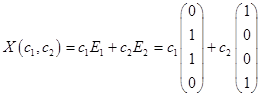
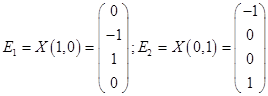
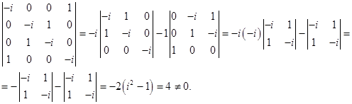
Число  есть собственное число оператора
  в том и только том случае, когда
  . Запишем характеристическое уравнение:
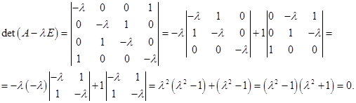
Решая его, имеем
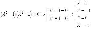
Таким образом, получаем собственные числа оператора:
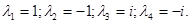
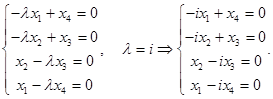
Для каждого из полученных собственных значений найдем собственные векторы.
Их можно найти их системы 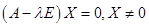 .
.
А) 
Решим однородную систему уравнений.
Матрица коэффициентов 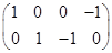 имеет ранг 2. Выберем в качестве базисного минора
  Тогда, полагая
  , имеем
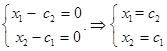
Таким образом, общее решение системы
 .
.
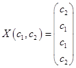
Из общего решения находим фундаментальную систему решений:
 .
.
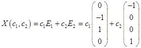
С использованием фундаментальной системы решений, общее решение может быть записано в виде .
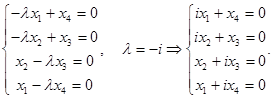
Б) 
Решим однородную систему уравнений
 .
.
Матрица коэффициентов  имеет ранг 2. Выберем в качестве базисного минора Тогда, полагая , имеем
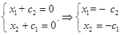
Таким образом, общее решение системы 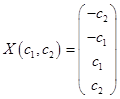 .
.
Из общего решения находим фундаментальную систему решений:
 .
.
С использованием фундаментальной системы решений, общее решение может быть записано в виде
 .
.
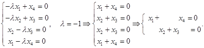
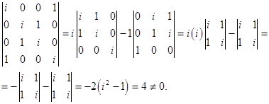
В) 
Решим однородную систему уравнений.
Матрица коэффициентов 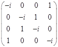 имеет ранг 4, поскольку
Так как ранг равен количеству неизвестных, то система имеет только тривиальное решение.
Г) 
Решим однородную систему уравнений.
Матрица коэффициентов  имеет ранг 4, поскольку
Так как ранг равен количеству неизвестных, то система имеет только тривиальное решение.
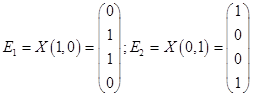
Таким образом, имеем собственные вектора 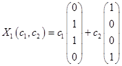 и
и 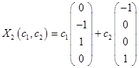 .
.
Выберем в качестве ортогонального базиса вектора  ,
,  ,
,  ,
,  .
.
Нормируем найденный ортогональный базис:
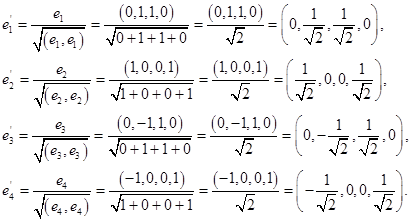
Ответ: 
Matrix Transformations
Frank E. Harris, in Mathematics for Physical Science and Engineering, 2014
5.7 Matrix Diagonalization
Another approach to the Hermitian matrix eigenvalue problem can be developed if we place the orthonormal eigenvectors of a matrix H as columns of a matrix V, with the ith column of V containing the ith orthonormal eigenvector xi of H, whose eigenvalue is λi. For simplicity, let’s assume H and the xi to be real, so V is an orthogonal matrix. If we then form HV, the ith column of this matrix product is λixi. Moreover, if we let Λ be a diagonal matrix whose elements Λii are the eigenvalues λi, we then see that the matrix product VΛ is a matrix whose columns are also λixi. This situation is illustrated schematically as follows:

corresponding to the equation
(5.37)HV=VΛ.
We now multiply Eq. (5.37) on the left by VT, obtaining the matrix equation
(5.38)VTHV=Λ.
Equation (5.38) has a nice interpretation. That equation has the form of a orthogonal transformation by the matrix VT. In other words, V is the inverse (and also the transpose) of the matrix U that rotates H into the diagonal matrix Λ. We therefore have the following important result:
A real symmetric matrix H can be brought to diagonal form by the transformation UHUT=Λ, where U is an orthogonal matrix; the diagonal matrix Λ has the eigenvalues of H as its diagonal elements and the columns of UT are the orthonormal eigenvectors of H, in the same order as the corresponding eigenvalues in Λ.
More casually, one says that a real symmetric matrix can be diagonalized by an orthogonal transformation.
The fact that the eigenvectors and eigenvalues of a real symmetric matrix can be found by diagonalizing it suggests that a route to the solution of eigenvalue problems might be to search for (and hopefully find) a diagonalizing orthogonal transformation. We cannot expect to find an explicit and direct matrix diagonalization method, because that would be equivalent to finding an explicit method for solving algebraic equations of arbitrary order, and it is known that no explicit solution exists for such equations of degree larger than 4. However, numerical methods have been developed for approaching diagonalization via successive approximations, and the insights of this section have contributed to those developments. Matrix diagonalization has been one of the most studied problems of applied numerical mathematics, and methods of high efficiency are now widely available for both numerical and symbolic computation. Already as long ago as 1990 researchers had published communications1 that report the finding of some eigenvalues and eigenvectors of matrices of dimension larger than 109. Extrapolating the increase in computer power to the date of publication of this text, an estimate of the largest matrix that could be handled in 2012 would be of a dimension somewhat larger than 1010.
Simultaneous Eigenfunctions
Because a quantum-mechanical system in a state which is an eigenvector of some Hermitian matrix A is postulated to have the corresponding eigenvalue as the unique definite value of the physical quantity associated with A, it is of great interest to know when it will also always be possible to observe at the same time a unique definite value of another quantity that is associated with a Hermitian matrix B. From a mathematical point of view, the question we are asking deals with the possibility that A and B have a complete common set of eigenvectors.
The key result here is simple:
Hermitian matrices have a complete set of simultaneous eigenvectors if and only if they commute.
For proof the reader is referred to Arfken et al in the Additional Readings.
It may happen that we have three matrices A,B, and C, and that [A,B]=0 and [A,C]=0, but [B,C]≠0. In that case, which is actually quite common in atomic physics, we have a choice. We can insist upon a set of vectors that are simultaneous eigenvectors of A and B, in which case not all of them can be eigenvectors of C, or we can have simultaneous eigenvectors of A and C, but not B. In atomic physics, those choices typically correspond to descriptions in which different angular momenta are required to have definite values.
Example 5.7.1 Simultaneous Eigenvectors
Consider the three matrices
A=1-100-110000200002,B=00000000000-i00i0,
C=00-i/2000i/20i/2-i/2000000.
The reader can verify that these matrices are such that [A,B]=[A,C]=0, but [B,C]≠0, i.e., BC≠CB. An orthogonal matrix U that diagonalizes A is
U=1/21/2001/2-1/20000100001;
when U is applied to A,B, and C, we get
UAUT=0000020000200002,UBUT=00000000000-i00i0,
UCUT=000000-i00i000000.
At this point, neither UBUT nor UCUT is also diagonal, but we can choose to diagonalize one of them (we choose UBUT) by a further orthogonal transformation that will modify the lower 3×3 block of UBUT (note that because this block of UAUT is proportional to a unit matrix the transformation we plan to make will not change it).
An orthogonal matrix V that diagonalizes UBUT is
V=10000100001/2i/2001/2-i/2;
as already stated, further transformation with V leaves UAUT unchanged, and converts UBUT and UCUT to
VUBUTVT=0000000000-100001,VUCUTVT=000000-i/2-i/20i/2000i/200.
The columns of UTVT=(VU)T are the simultaneous eigenvectors of A and B (but not C). It is not possible to diagonalize simultaneously both B and C, but we could have chosen to diagonalize C rather than B. ▪
Read full chapter
URL:
https://www.sciencedirect.com/science/article/pii/B9780128010006000055
Multivariate Analysis
P.K. Bhattacharya, Prabir Burman, in Theory and Methods of Statistics, 2016
Principal Factor Analysis
Let λ^1≥⋯≥λ^p be the eigenvalues of the sample covariance matrix S with the corresponding orthonormal eigenvectors û1,…,ûp. Then the p × k matrix L^=[λ^11/2û1,…,λ^k1/2ûk] is taken to be an estimate of L, that is, the columns of L^ are l^j=λ^j1/2ûj, j = 1, …, k, and hence L^L^T=∑j=1kλ^jûjûjT. Here
ĥi2=l^i12+⋯+l^ik2,ψ^i=sii−ĥi2,
where sii is the ith diagonal element of the sample covariance matrix S. An estimate of the proportion of total variability of Y explained by the first factor is ∥l^1∥2/trace(S)=λ^1/trace(S). In general, an estimate of the proportion of total variability of Y explained by the jth factor is λ^j/trace(S), j = 1, …, k.
If the sample correlation matrix is used in the analysis instead of the sample covariance matrix, then L^=[λ^11/2û1,…,λ^k1/2ûk], where λ^1≥λ^2≥⋯ are the eigenvalues of the sample correlation matrix with the corresponding normalized eigenvectors û1,û2,…. In this case, ĥi2=l^i12+⋯+l^ik2, ψ^i=1−ĥi2, and the proportion of the total variability explained by the jth factor is λ^j/p, j = 1, 2, … .
Read full chapter
URL:
https://www.sciencedirect.com/science/article/pii/B9780128024409000126
Classical and Quantum Information Theory
Dan C. Marinescu, Gabriela M. Marinescu, in Classical and Quantum Information, 2012
Theorem.
(Uhlmann) The fidelity of the two mixed quantum states, ρA and ρB, is equal to the maximum value of the modulus of the inner product of any purifications, |ϕA〉and|ϕB〉, respectively, of the two density matrices,
F(ρA,ρB)=max(ϕA,ϕB)〈ϕA|ϕB〉|2.
The proof discussed in this sections is due to Richard Jozsa [220] and avoids the difficulties of the original proof of Uhlmann [429] based on the representation theory of C* -algebras.
The two mixed states, ρA and ρB, are defined on an n-dimensional Hilbert space, Hn, and their purifications, |ϕA〉 and |ϕB〉, are defined on the extended space, Hn⊗Hn′. Without loss of generality, we assume that Hn′=Hn; thus, ϕA,ϕB∈Hn⊗Hn. We wish to express the two pure states, |ϕA〉 and |ϕB〉, in terms of the eigenvectors and eigenvalues of the corresponding density matrices, using Schmidt decomposition and
|ϕA〉=∑ipiA|ai〉⊗|ci〉 and |ϕB〉=∑ipiB|bi〉⊗|di〉.
In these expressions:
- 1.
-
A = {|a1〉, |a2〉,…, |an〉} is the set of orthonormal eigenvectors of ρA in Hn;p1A,p2A,…,pnA are the corresponding eigenvalues.
- 2.
-
B − {|b1>, |b2>,…,|bn>} is the set of orthonormal eigenvectors of ρB in Hn;p1B,p2B, …, pnB are the corresponding eigenvalues.
- 3.
-
C − {|c1〉, |c2〉,…, |cn>} and D = {|d1〉, |d2〉,…, |dn〉} are two orthonormal bases in H′n.
There are some unitary transformations, B, C, and D, that allow us to express the orthonormal bases, B, C, and D, as follows:
|bi〉=B|ai〉,|ci〉=C|ai〉, and |di〉=D|bi〉.
We also observe that
piA=ρA and piB=ρB.
Now we express the two pure states as
|ϕA}=∑ipiA|ai}⊗|ci}=[ρA⊗I]∑i|ai}⊗C|ai}=∑iρAC†|ai}⊗|ai}
and
|ϕB〉=∑jpjB|bj〉⊗|dj〉=∑jρBD†|bj〉⊗|bj〉=∑jρBD†B|aj〉⊗B|aj〉=ρBD†[B⊗I]∑j|aj〉⊗B|aj〉=∑jρBD†BB†|aj〉⊗|aj〉.
Finally,
〈ϕA|ϕB〉=∑i〈ai|C†ρAρBD†BB†|ai〉=tr(ρAρBD†BB↑C†).
It follows that the maximum value of |〈ϕA|ϕB〉| is tr (|ρAρB|) as B, C, and D are unitary transformations. We also can write
|ρAρB|=((ρAρB)(ρAρB)†)1/2=(ρAρBρBρA)1/2=(ρAρBρA)1/2.
We conclude that F (ρA, ρB)=max(ϕA,ϕB)|〈ϕA|ϕB〉|2.
Read full chapter
URL:
https://www.sciencedirect.com/science/article/pii/B9780123838742000035
Canonical Correlation
A. Basu, A. Mandal, in International Encyclopedia of Education (Third Edition), 2010
Canonical Correlations
Let X represent the first set of variables, and let Y denote the second set of variables. Assume that X is m dimensional, and let the dimension of Y be n. Without loss of generality, let m ≤ n. Let Cov(X), Cov(Y) and Cov(X, Y) be denoted by ∑11m×m, ∑22n×n, and ∑12m×n, respectively, with the superscripts denoting the dimensions of the matrices. We will drop the superscripts when there is no scope for confusion. We will assume that the (m + n) × (m + n) dimensional square matrix
∑=(∑11∑12∑21∑22)
is positive definite, where ∑21=∑12T. We will generalize the concept of multiple correlation and describe the correlation structure resulting from the elements of Σ in terms of appropriately chosen pairs of canonical variables.
We will consider linear combinations of the form
[1]U1=a1TXandV1=b1TY
where a1 and b1 are m and n dimensional coefficient vectors, respectively. From standard statistical theory, we have
Var(U1)=a1T∑11a1,Var(V1)=b1T∑22b1andCov(U1,V1)=a1T∑12b1
Thus, the correlation between the variables U1 and V1 is given by
[2]Corr(U1,V1)=a1T∑12b1a1T∑11a1b1T∑22b1
Our aim is to choose a1 and b1 to maximize the above correlation. The quantity
[3]maxa1,b1Corr(U1,V1)
obtained as a result of the above maximization will be referred to as the first canonical correlation between the sets X and Y, and the corresponding variable pair will be denoted as the first canonical variable pair. Later we will continue the description in terms of the second, third, and subsequent canonical variable pairs.
The development of the canonical correlations will require a few mathematical tools involving eigenvalues and eigenvectors of nonnegative definite matrices, which we state in the following (without proofs). The proofs are available in most standard texts of linear algebra or applied multivariate analysis. Johnson and Wichern (2006), for example, is a typical reference.
Lemma 1: Suppose A is a p × p nonnegative definite matrix having eigenvalues λ1≥⋯≥λj≥⋯≥λp, with corresponding orthonormal eigenvectors e1, … ,ej, … ,ep.
- (i)
-
Let s be any p dimensional vector. We are interested in the maximum value of the normalized quadratic form in A over all non-null vectors s. This maximum is given by
[4]maxs≠0sTAssTs=λ1
where λ1 is the largest eigenvalue of A. The maximum is attained when s = e1.
- (ii)
-
Among all nonnull p dimensional vectors s which are orthogonal to e1, … ,e(j − 1), j = 2, … ,p, the same maximization problem leads to
[5]maxs⊥e1,…,e(j−1)sTAssTs=λj
and this maximum is attained at s = ej.
Define the matrices M and N as
[6]M=∑11−1/2∑12∑22−1∑21∑11−1/2andN=∑22−1/2∑21∑11−1∑12∑22−1/2
where ∑11−1/2 and ∑22−1/2 are positive definite square roots of ∑11−1 and ∑22−1, respectively. Notice that the matrix M can be written in the form BBT where B=Bm×n=∑11−1/2∑12∑22−1/2, and hence M is non-negative definite. Similarly, N can be written as BTB, and hence N is non-negative definite as well. This representation also shows that the set of nonzero eigenvalues of M and N are the same (this is a consequence of the eigenvalues of CD and DC being the same, wherever the multiplication of the matrices C and D, and D and C, are defined); in particular if ρ1 is the largest eigenvalue of M, it is also the largest eigenvalue of N. Also if e is a normalized eigenvector of M corresponding to some nonzero eigenvalue ρ, then BTe is an eigenvector of N associated with the eigenvalue ρ; division by ρ reduces the length of this eigenvector to 1. Thus,
[7]f=BTe/ρ
is a normalized eigenvector of N associated with the eigenvalue ρ.
With this background, we are now ready to state and prove the following theorems.
Theorem 1: The elements of the first canonical variable pair (U1, V1) are given by
U1=e1T∑11−1/2XandV1=f1T∑22−1/2Y
where e1 and f1 are the normalized eigenvectors associated with the largest eigenvalue ρ1 of M and N, respectively. The value of the first canonical correlation is ρ1.
Proof: We consider linear combinationsU1=a1TX and V1=b1TY with the aim of maximizing Corr(U1, V1) over a1 and b1. Let c1=∑111/2a1 and d1=∑221/2b1. Using eqn [2], we can represent the correlation coefficient between U1 and V1:
[8]Corr(U1,V1)=a1T∑12b1a1T∑11a1b1T∑22b1=c1T∑11−1/2∑12∑22−1/2d1c1Tc1d1Td1
By a simple application of the Cauchy–Schwarz theorem, we observe that the numerator on the right-hand side of the quantity in eqn [8] is bounded above by
(c1T∑11−1/2∑12∑22−1/2∑21∑11−1/2c1)1/2(d1Td1)1/2
and the substitution of this in eqn [8] gives
[9]Corr(U1,V1)≤(c1T∑11−1/2∑12∑22−1/2∑21∑11−1/2c1)1/2(c1Tc1)1/2=(c1TMc1)1/2(c1Tc1)1/2≤ρ1
The last inequality follows from eqn [4]. Thus, Corr(U1, V1) is bounded by ρ1, where ρ1 is the largest eigenvalue of M.
It remains to show that Corr(U1, V1) attains this bound for the particular choices a1=∑11−1/2e1 and b1=∑22−1/2f1. Since e1 and f1 are normalized eigenvectors, direct substitution of the expressions in eqn [8] gives
[10]Corr(U1,V1)=(e1T∑11−1/2∑12∑22−1/2f1)(e1Te1)(f1Tf1)=e1TBf1
An application of eqn (7) shows
[11]Corr(U1,V1)=e1TBBTe1ρ1=e1TMe1ρ1=ρ1e1Te1ρ1=ρ1
which establishes the desired result.
The last part of the proof can also be shown by checking that these particular choices of a1 and b1 lead to equalities in both the inequalities of eqn [9].
Notice that since we are maximizing a correlation which is a scale-independent measure, the value of the correlation would remain the same if the coefficient vectors a1 and b1 were multiplied by any scalar constants. The particular choice given here ensures that the variance of the variables U1 and V1 are equal to unity. This is presented more formally later in Theorem 3.
Theorem 2: The jth pair of canonical variables (Uj, Vj), j = 2, …, m, are given by
Uj=ejT∑11−1/2XandVj=fjT∑22−1/2Y
where ej and fj are the orthonormal eigenvectors associated with the jth largest eigenvalue ρj of M and N. The jth canonical correlation is given by CorrUj,Vj=ρj.
Proof: We will determine linear combinations U2=a2TX and V2=b2TY such that Corr(U2, V2) is maximized subject to Cov(U1, U2) = Cov(V1, V2) = 0. By denoting a2=∑11−1/2c2 and b2=∑22−1/2d2, we get
Cov(U1,V1)=Cov(e1T∑11−1/2X,c2T∑11−1/2X)=eT∑11−1/2∑11∑11−1/2c2
Thus, Cov(U1, U2) = 0 implies that c2 must belong to the orthogonal space of e1. Similarly, d2 can be shown to belong to the orthogonal space of f1.
Therefore, we will have to maximize
[12]Corr(U2,V2)=c2T∑11−1/2∑12∑22−1/2d2c2Tc2d2Td2
subject to the restrictions on c2 and d2. As in Theorem 1, an application of the Cauchy–Schwarz inequality gives
[13]Corr(U2,V2)≤(c2TMc2)1/2(c2Tc2)1/2≤ρ2
where the last inequality follows from Lemma 1 (ii). Direct substitution shows that equality is attained for c2=∑11−1/2e2 and d2=∑22−1/2f2.
The result for the successive canonical correlations can be proved in a similar fashion.
Theorem 3: The canonical variable pairs have the properties
[14]Var(Uj)=Var(Vj)=1,j=1,…,m
[15]Cov(Uj,Uk)=Corr(Uj,Uk)=0,j≠k
[16]Cov(Vj,Vk)=Corr(Vj,Vk)=0,j≠k
[17]Cov(Uj,Vk)=Corr(Uj,Vk)=0,j≠k
Proof: Property [14] is easily verifiable from the definition of the canonical variables, and properties [15] and [16] follow from the construction of the canonical correlation pairs as outlined in Theorem 2. For property [17], note that
Cov(Uj,Vk)=ejT∑11−1/2∑12∑22−1/2fk=ejTMek/ρk=0
The last inequality follows from the fact that the vectors ej and ek are orthonormal eigenvectors of M. The previous equality follows from eqn [7].
In real situations where actual data are generated from the variables of interest, the theoretical quantities in the setup described in Theorems 1–3 are replaced by their sample analogs. Thus, for example, the population covariance matrix Σ will be replaced by the sample covariance matrix S.
Read full chapter
URL:
https://www.sciencedirect.com/science/article/pii/B9780080448947013105
Advancements in Bayesian Methods and Implementation
Geethu Joseph, … Sai Subramanyam Thoota, in Handbook of Statistics, 2022
7.3.1 SBL-based algorithms in the presence of colored noise
Let us consider the case where Q is known. We decompose Q using the eigenvalue decomposition as Q=VΛV⊺, where the columns of V∈Rm×m contain the orthonormal eigenvectors of Q, and the diagonal matrix Λ contains the eigenvalues of Q. When the rank of Q is p (≤ m), it can be decomposed as:
(86)Q=[V1V2]D0p×m−p0m−p×p0m−p×m−pV1⊺V2⊺,
where 0p×m represents a p × m all zero matrix, and D is a diagonal matrix containing the p nonzero eigenvalues of Q. By premultiplying the observations Y by V1⊺ and V2⊺, we get the projected observations Yi = AiX + Wi, where Yi=Vi⊺Y, Ai=Vi⊺A, and Wi=Vi⊺W. Under this projection, W1 has a diagonal, full rank covariance matrix D, while W2 = 0m−p×L. Our problem thus reduces to the recovery of sparse signals from a mixture of noisy and noiseless measurements. EM-based algorithms can be employed to solve the above problem.
Read full chapter
URL:
https://www.sciencedirect.com/science/article/pii/S0169716122000414
Functional Analysis
C.W. Groetsch, in Encyclopedia of Physical Science and Technology (Third Edition), 2003
IV.B The Spectral Theorem
We limit our discussion of the spectral theorem to the case of a compact self-adjoint operator. The spectral theorem gives a particularly simple characterization of the range of such an operator. We have seen that the nonzero eigenvalues of a compact self-adjoint operator T of infinite rank form a sequence of real numbers {λn} with λn → 0 as n → ∞. The corresponding eigenspaces N(T − λnI) are all finite-dimensional and there is a sequence {υn} of orthonormal eigenvectors, that is, vectors satisfying
∥υj∥=1,〈υi,υj〉=0,fori≠j,and,Tυj=λjυj.
The closure of the range of T is the closure of the span of this sequence of eigenvectors. Since T is self-adjoint, N(T)⊥=R(T)¯ the decomposition theorem then gives the representation
w=Pw+∑j=1∞〈w,υj〉υj
for all w ∈ H, where P is the projection operator from H onto N(T). The range of T then has the form
Tw=∑j=1∞λj〈w,υj〉υj.
This result is known as the spectral theorem. It can be extended (in terms of a Stieljes integral with respect to a projection valued measure on the real line) to bounded self-adjoint operators (and beyond).
Read full chapter
URL:
https://www.sciencedirect.com/science/article/pii/B0122274105002696
Toda Lattices
Y.B. Suris, in Encyclopedia of Mathematical Physics, 2006
Moser’s Solution
Integration of this system has been first performed by J Moser in 1975. His solution can be interpreted within the general scheme of the IST (see Figure 1). The spectral data in this case consist, for example, of the eigenvalues μj(j=1,…,N) of the matrix L0 and the first components rj of the corresponding orthonormal eigenvectors. The evolution of these data induced by the Toda flow [2] turns out to be simple:
[29]μj=const.,rj2(t)=rj2(0)eμjtΣi=1Nri2(0)eμit
The IST is expressed by the identity
[30]∑j=1Nrj2μ−μj=1μ−b1−a1μ−b2−⋱−aN−1μ−bN
both parts of which represent the entry (1,1) of the matrix (μI−L0)−1. It implies that all variables an(t),bn(t) are rational functions of μj and eμjt; in particular, one finds:
[31]an(t)=eqn+1(t)−qn(t)=τn−1(t)τn+1(t)τn2(t)
where τn(t) can be represented as an n×n Hankel determinant
[32]τn(t)=det(cj+k(t))0≤j,k≤n−1cj(t)=∑i=1Nμijri2(t)
Read full chapter
URL:
https://www.sciencedirect.com/science/article/pii/B0125126662001899
Discrete Systems
In Modelling of Mechanical Systems, 2004
NOTE Hilbert’s spaces
More generally, a vector space which is complete (i.e. any Cauchy sequence converges to a vector within that space, for further details see Appendix 1 paragraph A1.4) and which is provided with a scalar product is termed a Hilbert’s space. The scalar product is used to define the natural metrics of the space.
Returning back to matrices operating on a Hilbert’s space of finite dimension, it is recalled that the eigenvalues and the related eigenvectors of a matrix are the nontrivial solutions of the following homogeneous problem:
[2.35][[A]−λn[I]][Vn]=[0];with‖[Vn]‖≠0
where [I] denotes the identity matrix Ij,k =1, if j = k and 0 otherwise.
[φn] is the n-th eigenvector of [A] which is related to the n-th eigenvalue λn. The natural norm of [φn] is
‖[φn]‖=〈φn,φn〉. Unit eigenvectors are then produced by using the natural norm.
Hermitian matrices have the properties which are listed below (for mathematical proofs, see Appendix 4):
- 1.
-
All the eigenvalues are real numbers.
- 2.
-
All the eigenvectors related to distinct eigenvalues are orthogonal to each others.
- 3.
-
Starting from the whole set of eigenvectors, it is always possible to define an orthonormal basis of the Hilbert’s space in which [H] is operating. This basis is characterized by the transformation matrix [Φ], of which columns are formed with a set of N orthonormal eigenvectors. Therefore [Φ] is said to be orthonormal and it can be shown that its inverse is identical to its adjoint:
[2.36][Φ]−1=[Φ*]T
The matrix [Φ] can be used to transform [H] into a diagonal form as follows:
[2.37][Λ]=[Φ]−1[H][Φ]=[Φ*]T[H][Φ];Λij=λiifj=iand0otherwise
In the language of geometry, the transformation [2.37] is a similarity. Similarity maintains the parallelism of vectors, but not the direction. Two matrices related to each other by similarity are said to be similar. The eigenvalues of similar matrices are the same.
- 4.
-
The orthonormal transformation [Y] = [Φ][X] can also be viewed as an orthonormal change of coordinates of the same vector from the initial basis of definition (coordinates qn) to the basis of the [φn] (coordinates q ‘n). The transformation of coordinates is written as:
[2.38][q]=[Φ][q’]⇔[q’]=[Φ]−1[q]=[Φ*]T[q]
Any [H] matrix is thus transformed into a similar matrix noted [H]′:
[2.39][H]′=[Φ*]T[H][Φ]
Going back now to the special case of symmetrical matrices [S] operating in a real vector space, we consider the quadratic form:
[2.40][q]T[S][q]=σ
If the sign of σ remains the same whichever [q] may be, except the null vector, [S] is said to be either positive definite, or negative definite, in accordance with the sign of σ. Now it can be shown that the necessary and sufficient condition for [S] to be of a given sign is that all the eigenvalues are of the same sign, i.e. positive if [S] is positive. Obviously, two other cases are also possible. One is that all the eigenvalues have the same sign, except some of them, which are found to be zero. Such a matrix is said to be positive, or negative, in accordance with the sign of the nonvanishing eigenvalues. A final occurrence is that all the eigenvalues do not have the same sign, in which case the sign of the matrix is undefined.
Read full chapter
URL:
https://www.sciencedirect.com/science/article/pii/S1874705101800050
Eigenvalue Problems
George B. Arfken, … Frank E. Harris, in Mathematical Methods for Physicists (Seventh Edition), 2013
Spectral Decomposition
Once the eigenvalues and eigenvectors of a Hermitian matrix H have been found, we can express H in terms of these quantities. Since mathematicians call the set of eigenvalues of H its spectrum, the expression we now derive for H is referred to as its spectral decomposition.
As previously noted, in the orthonormal eigenvector basis the matrix H will be diagonal. Then, instead of the general form for the basis expansion of an operator, H will be of the diagonal form
(6.25)H=∑μ|cμ〉λμ〈cμ|, each cμ satisfies Hcμ=λμcμ and〈cμ|cμ〉=1.
This result, the spectral decomposition of H, is easily checked by applying it to any eigenvector cν.
Another result related to the spectral decomposition of H can be obtained if we multiply both sides of the equation Hcμ = λμcμ on the left by H, reaching
H2cμ=(λμ)2cμ;
further applications of H show that all positive powers of H have the same eigenvectors as H, so if f (H) is any function of H that has a power-series expansion, it has spectral decomposition
(6.26)f(H)=∑μ|cμ〉f(λμ)〈cμ|.
Equation (6.26) can be extended to include negative powers if H is nonsingular; to do so, multiply Hcμ = λμcμ on the left by H−1 and rearrange, to obtain
H−1cμ=1λμcμ,
showing that negative powers of H also have the same eigenvectors as H.
Finally, we can now easily prove the trace formula, Eq. (2.84). In the eigenvector basis,
(6.27)det exp(A) =∏μeλμ=exp∑μλμ=exp trace(A) .
Since the determinant and trace are basis-independent, this proves the trace formula.
Read full chapter
URL:
https://www.sciencedirect.com/science/article/pii/B9780123846549000062
Preliminaries
Dan C. Marinescu, Gabriela M. Marinescu, in Classical and Quantum Information, 2012
Proof.
We calculate the inner product, 〉ψ| A|ψ〉, where λψ is the eigenvalue corresponding to the eigenvector | ψ〉 of A:
〈ψ|A|ψ〉=〈ψ|[A|ψ〉]=ψ|[λψ|ψ〉]=λψ〈ψ|ψ〉.
If we take the adjoint of A, |ψ〉=λψ|ψ〉, and use the fact that A is Hermitian, A = A†, it follows that 〉ψ|A=λψ*〉ψ|. We now rewrite the inner product:
〈ψ|A|ψ〉=[〈ψ|A]|ψ〉=ψ|[λψ*〈ψ|]|ψ〉=λψ*〈ψ|ψ〉.
It follows that
λψ〈ψ|ψ〉=λψ*〈ψ|ψ〉⇒=(λψ-λψ*)〈ψ|ψ〉=0,∀|ψ〉∈Hn.
Since 〈ψ|ψ〉≠0, it follows that λψ=λψ* thus, the eigenvalue λψ is a real number.
P2. Two eigenvectors, |ψ〉 and |φ〉, of the Hermitian operator A with the distinct eigenvalues, λψ ≠ Xψ, are orthogonal, 〈ψ | ψ〉 = 0.
Proof.
We calculate the inner product, 〈ψ | A | ψ〉, and use the fact that λψ is an eigenvalue of A corresponding to the eigenvector, λψ≠λψ thus, A 〈ψ|φ〉:
〈ψ|A|φ〉=〈ψ|[A|φ〉]=〈ψ|[λψ|φ〉]=λψ〈ψ|φ〉.
The eigenvalue λψ corresponds to the eigenvector | ψ〉; thus, A | ψ〉 = λψ | ψ〉. If we take the adjoint of this expression and use the fact that A is Hermitian, A = A†, it follows that 〈ψA=*ψ〈ψ|. We can now rewrite the inner product:
〈ψ|A|φ〉=[〈ψ|A]|φ〉=[λψ*〈ψ|]|φ〉=λψ*〈ψ|φ〉.
It follows thatλφ〈ψ|φ〉=λψ*〈ψ|φ〉∀λψ≠λφ.
This is possible if and only if 〈ψ|φ〉= 0.
P3. For every Hermitian operator A there exists a basis of orthonormal eigenvectors such that the matrix A is diagonal in that basis and its diagonal elements are all the eigenvalues of A.
Proof.
Let |ψ〉, 1 ≤ i ≤ n, be an eigenvector of A and λi the corresponding eigenvalue. If the eigenvalues are distinct, λi ≠ λj for i ≠ j, 1 ≤ i,j ≤ n, we construct the orthonormal basis as follows: we select an eigenvector | ψj〉 from a subspace that is orthogonal to the subspace spanned by (|ψ1,|ψ2〉,…,|ψi〉).
Then:A=(λ100……0λ20……00λ3……⋮⋮⋮⋱⋮⋮⋮λn)..
If the eigenvalues, λj, are degenerate (not distinct), then there are many bases of eigenvectors that diagonalize matrix A. If λ is an eigenvalue of multiplicity K < 1, the set of corresponding eigenvectors generates a subspace of dimension K, the eigenspace corresponding to that λ; the eigenspaces corresponding to different eigenvalues are orthogonal. Assume that λ is a degenerate eigenvalue, and the corresponding eigenvectors are | ψλ1 〉 and | ψλ2〉:
A|ψλ1〉=λ|ψλ1〉 and A|ψλ2〉=λ|ψλ2〉.
Then, ∀α1, α2ɛ ℂ:
A (a1|ψλ1〉+a2|ψλ2〉)=λ(a1|ψλ1〉+a2|ψλ2〉).
We can say that there is a whole subspace spanned by the vectors, | ψλ1〉 and | ψλ2〉, the elements of which are eigenvectors of A, with eigenvalues λ.
P4. The necessary and sufficient condition for two Hermitian operators, A1 and A2, to have the same set of eigenvectors is that they commute with each other:
[A1,A2]=A1A2-A2A1=0.
P5. The eigenvectors of a projector operator, Pψ = |ψ〉〈ψ|, where 〈ψ|ψ〉 = 1, are either perpendicular or collinear to the vector | ψ〉 and their eigenvalues are 0 and 1, respectively.
Proof.
Assume | ψ〈 is an eigenvector of Pψ corresponding to the eigenvalue λ:
Pψ〉φ}=λ|φ〉
or
|ψ〉〈ψ|φ〉=λ|φ〉.
The inner product, 〈ψ|φ〉, is a number γ :
λ|ψ〉=λ|φ〉.
This implies that
λ=0if V =0,when |ψ〉and|φ〉are perpendicular
or
λ=1if V=1,when |ψ〉and|φ〉are parallel and normalized.▪
An operator A is unitary if AnA†n = A†nAn= InClearly, a unitary operator is normal. The product of unitary operators is unitary, but the sum is not; “product” in this case means composition, not to be confused with tensor product.
A unitary operator A preserves the inner product; thus, it preserves the distance in a Hilbert space. If |ψ1〉,|ψ2〉,|φ1〉 ɛHn|φ1〉=A|ψ1〉 and |φ2〉=A|ψ2〉, then:
〈φ1|φ2〉=〈ψ1|ψ2〉.
Indeed, the inner product, 〈ψ1 | ψ2〉, can be written as
〈φ1|φ2〉=[A|ψ1〉]†A|ψ2〉=〈ψ1|A†A|ψ2〉=〈ψ1|ψ2〉.
It follows immediately that a unitary operator A preserves the norm of a vector:
[〈φ|A†][A|φ〉]={φ|[A†A]|φ〉=〈φ|φ〉.
If A is a unitary operator, then we can undo its action (i.e., a unitary operator is invertible and A−1 = A†).
Every normal operator has a complete set of orthonormal eigenvectors. If | ei〉 is an eigenvector (eigenstate) of the operator A and λi is the associated eigenvalue, then we can write
A |ei〉=λi|ei〉.
The spectral decomposition of a normal operator A is
A=∑iλiPi,
with Pi = ei〉〈ei, the projector corresponding to the eigenvector | ei〉.
Proof.
Note that (A + A†)/2 and (A − A†)/2i are Hermitian and commute. By P3 and P4 there exists an orthonormal base, {|e1〉,|e2〉,…,|en〉}, of eigenvectors simultaneously for (A + A†)/2 and (A − A†)/2i. Hence, they are also eigenvectors forA=(A+A↑2+iA-A↑2i)
Let λ1,λ2, …, λn be the eigenvalues corresponding to the eigenvectors {|e1〉|e2〉,…,|en〉}:
α=∑iλiΡi, with Ρi=|ei〉〈ei|.
Indeed, both A and ∑iλiΡi have the same matrix representation with respect to the base {|e1〉,|e2〉,…,|en〉}.
Example. Choose an orthonormal basis in H2. Let A be a 2 × 2 matrix in this basis:
A=(a11a12a21a22).
Calculate its eigenvalues, λ1 and λ2, possibly equal. Find linearly independent solutions of the two linear equations:
A(x1y1)=λ1(x1y1)and A(x2y2)=λ2(x2y2).
Define
| v1=(y1|x1|2+|y1|2×1|x1|2+|y1|2)and|v2〉=(y2|x2|2+|y2|2×2|x2|2+|y2|2).
The vectors, |v1〉 and |v2〉, form another basis for A, such that we can express A as
A =λ1|v1〉〈V1|+λ2|v2〉〈V2|.
Now we introduce the concept of positive operators and define the square root and the modulus of a positive operator; then we describe the canonical decomposition of an invertible operator [354].
Read full chapter
URL:
https://www.sciencedirect.com/science/article/pii/B9780123838742000011