#статьи
- 6 окт 2022
-

0
Стыдные вопросы о логарифмах: всё, что нужно знать программисту
Объясняем, почему не стоит бояться логарифмов и как их считать в Python.
Иллюстрация: Оля Ежак для Skillbox Media

Журналист, изучает Python. Любит разбираться в мелочах, общаться с людьми и понимать их.
Прежде чем начать обсуждение, давайте немного освежим знания и решим несколько стандартных задачек:
- Чему равен log3 81?
- А lg 2 × lb 10?
- А сумма log216 2 + log216 3?
Если вы легко прорешали все три примера в уме, не пользуясь калькулятором, — можете сразу переходить к заключительной главе. Для тех же, кто слегка подзабыл школьные годы чудесные, — буквально пять минут ликбеза.
По большому счёту, логарифм — это просто перевёрнутая степень. Рассмотрим выражение 23 = 8. В нём:
- 2 — основание степени;
- 3 — показатель степени;
- 8 — результат возведения в степень.
У возведения в степень существует два обратных выражения. В одном мы ищем основание (это извлечение корня), в другом — показатель (это логарифмирование).
Таким образом, выражение 23 = 8 можно превратить в log2 8 = 3.
Закрепляем знания: логарифм — это число, в которое нужно возвести 2 (основание степени), чтобы получить 8 (результат возведения в степень).
Форма записи неинтуитивна, и поначалу можно легко спутать основание со степенью. Чтобы избежать этого, можно использовать следующее правило:
Основание у логарифма, как и у возведения в степень, находится внизу.
Чтобы лучше запомнить структуру записи, посмотрите на эти выражения и постарайтесь понять их смысл:
- log3 9 = 2
- log4 64 = 3
- log5 625 = 4
- log7 343 = 3
- log10 100 = 2
- log2 128 = 7
- log2 0,25 = −2
- log625 125 = 0,75
В общем виде запись logAB читается так: логарифм B по основанию A.
Главная часть любого логарифма — его основание. Именно наличие общего основания у нескольких логарифмических функций позволяет проводить с ними различные операции.
Основанием натурального логарифма является число Эйлера (e) — иррациональное число, приблизительно равное 2,71828.
На всякий случай напомним, что такое иррациональные числа. Так называют числа, которые нельзя записать в виде обыкновенной дроби с целыми числителем и знаменателем. При этом знаменатель не должен быть равен нулю.
Например, 0,333… — рациональное число, потому что его можно записать как 1/3. А вот число Пи или корень из 2 — иррациональны.
Так как натуральные логарифмы часто используются, для них ввели особый способ записи: ln x — это то же самое, что loge x.
Представим кристалл, который весит 1 кг и растёт со скоростью 100% в год. Можно ожидать, что через год он будет весить 2 кг, но это не так.
Каждая новая выращенная часть начнёт растить свою собственную. Когда в кристалле будет 1,1 кг, он будет расти со скоростью 1,1 кг в год, а когда в нём будет 1,5 кг — со скоростью 1,5 кг в год. Математики подсчитали, что через год масса кристалла составит e, или ≈ 2,71828 кг.
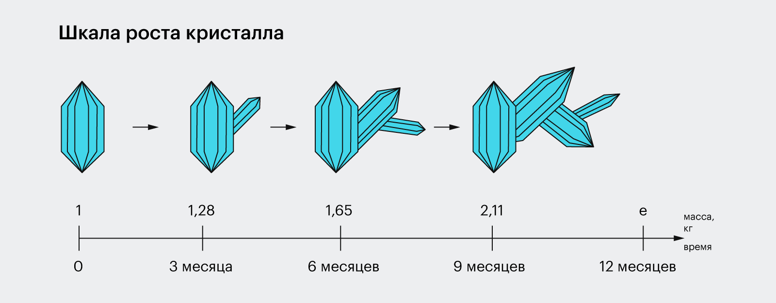
Такой рост называется экспоненциальным. По экспоненте размножаются бактерии, увеличиваются популяции, приумножаются доходы, растут снежные комья, распадается радиоактивное вещество и остывают напитки.
Чтобы узнать, какой массы достигнет кристалл через три, пять, десять лет, нужно возвести e в соответствующую степень.
e3 ≈ 20,0855 кг
e5 ≈ 148,4132 кг
e10 ≈ 22 026,4658 кг
Но как рассчитать, когда кристалл будет весить тонну? Составим уравнение:
ex = 1000
Нам известны основание степени и результат возведения в степень — осталось найти её показатель. Ничего не напоминает? Это ведь и есть логарифм x = loge 1000! Или, если использовать сокращённую запись, x = ln 1000.
Подставим в калькулятор и выясним, что x ≈ 6,9. Именно столько лет потребуется кристаллу, чтобы его масса достигла тонны.
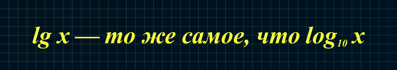
Десятичный логарифм — логарифм, основание которого равно 10. Он обозначается lg x и очень удобен, потому что с ним легко вычислять круглые числа.
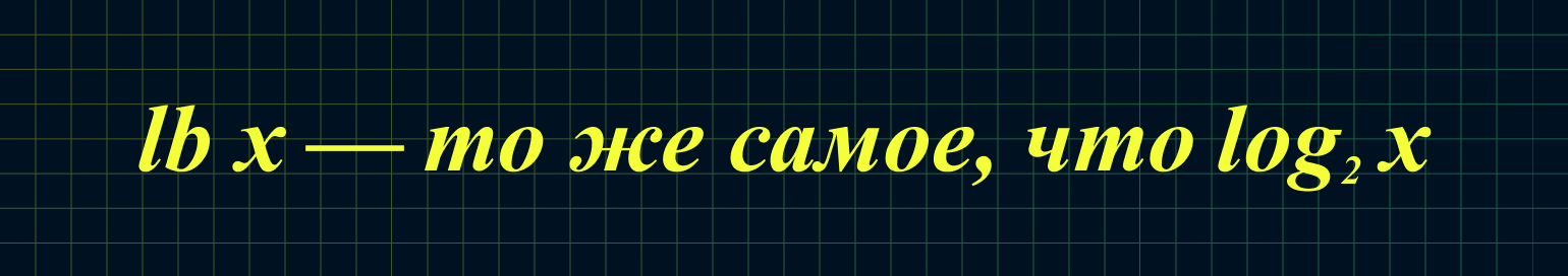
Двоичный логарифм — логарифм, основание которого равно 2. Он обозначается lb x и часто используется программистами, потому что компьютеры думают и считают в двоичной системе.
Список операций, которые можно совершать с логарифмами, ограничен. Если вы запомните все и научитесь их выполнять, то сможете щёлкать логарифмические задачки, как семечки.
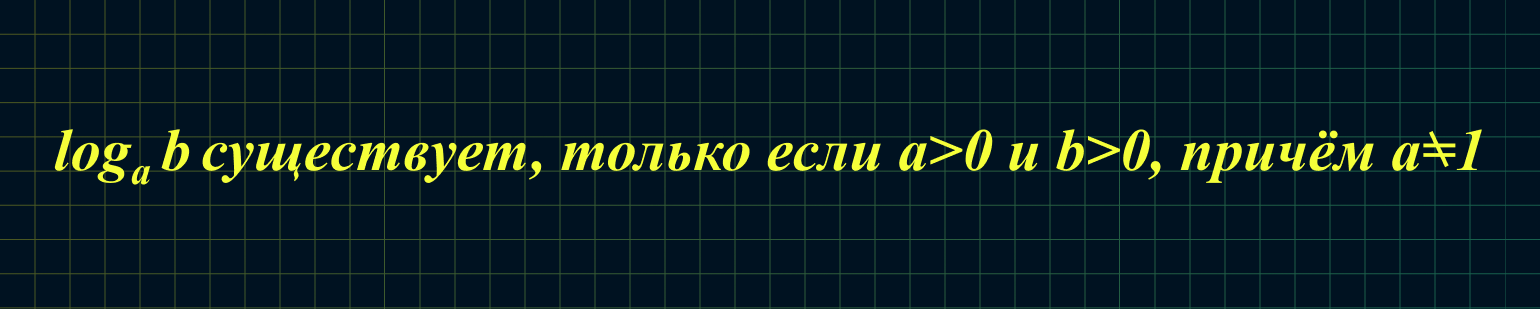
У всех логарифмов есть ограничения. Их основание и аргумент должны быть больше нуля, при этом основание не может быть равно единице. На математическом языке это звучит так:
Перейдём к свойствам логарифмов. Они работают в обе стороны, и их применяют как слева направо, так и справа налево.
1. Логарифм единицы по любому основанию всегда равен нулю:

Например: log17 1 = 0
2. Логарифм, где число и основание совпадают, равен единице:

Например: log17 17 = 1
3. Основное логарифмическое тождество:

Например: log17 175 = 5
4. Логарифм произведения чисел равен сумме их логарифмов:
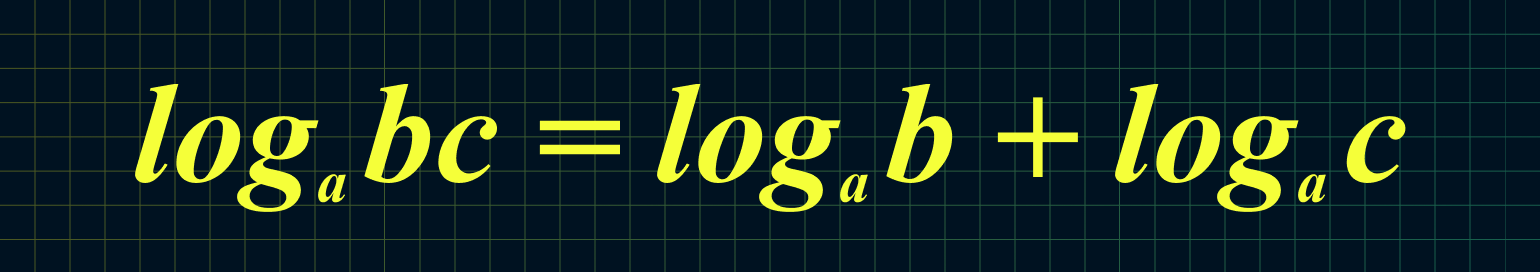
Например: log5 12,5 + log5 10 = log5 (12,5 × 10) = log5 125 = 3
5. Логарифм дроби равен разности логарифмов числителя и знаменателя:
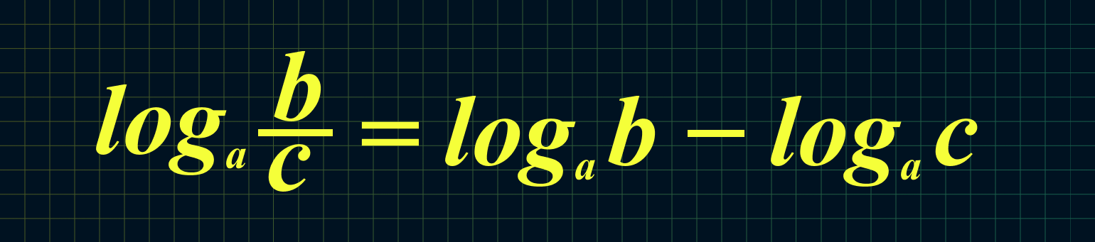
Например: log3 63 − log3 7 = log3 63/7 = log3 9 = 2
6. Если основание или аргумент возведены в степень, то их можно удобно выносить перед логарифмом:
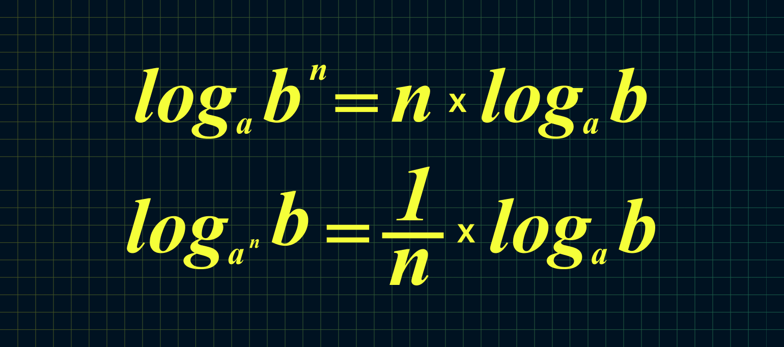
Из этих двух формул следует:
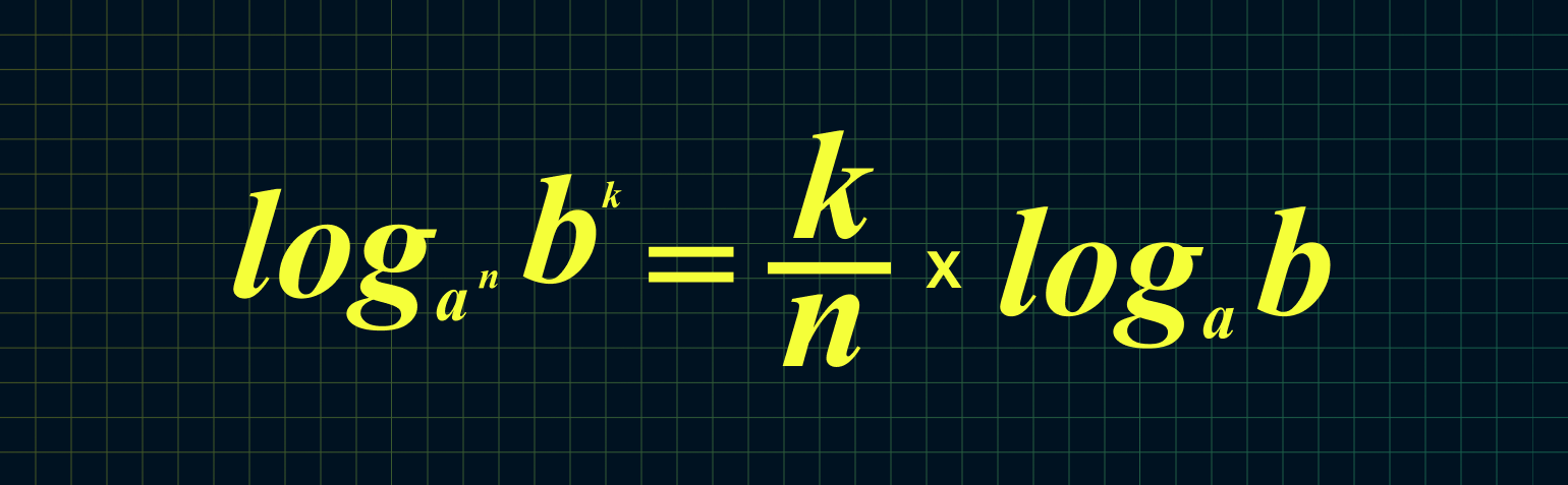
Например: log23 49 = 9/3 × log2 4 = 3 × 2 = 6
7. Если нам неудобно основание логарифма, то его можно изменить:
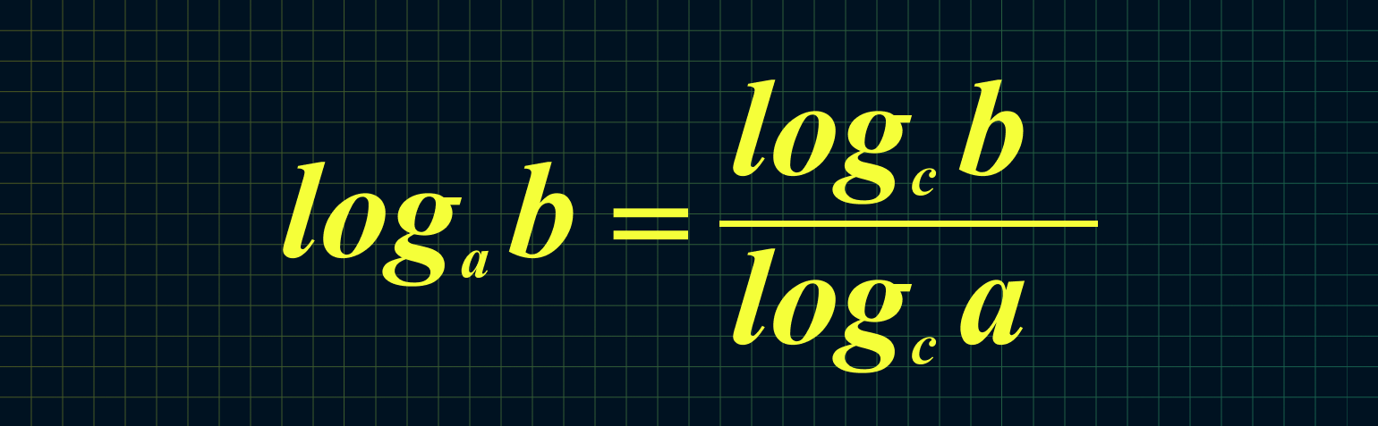
Например: log25 125 = log5 125/log5 25 = 3/2 = 1,5
Из этой формулы следует, что мы можем поменять местами основание и аргумент вот так:
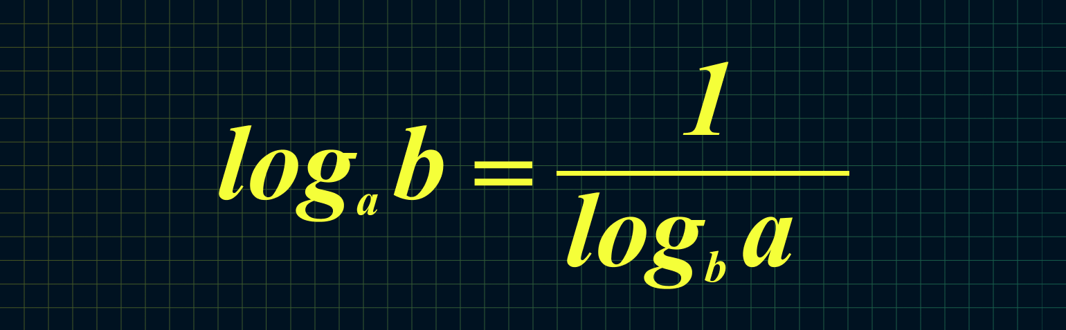
Например: log16 4 = 1/log4 16 = 1/2 = 0,5
А теперь возвращаемся к задачам, которые мы дали в начале статьи.
Пример 1
log3 81
Вспомните, что 81 — это 92. А 9 — это 32. Таким образом:
log3 81 = log3 92 = log3 32+2 = log3 34
Теперь логарифм не представляет для нас никаких сложностей. Воспользуемся свойством степени и вынесём четвёрку.
log3 34 = 4 × log3 3 = 4 × 1 =4
Ответ: 4.
Пример 2
lg 2 × lb 10
Переведём сокращённые записи в полный вид:
lg 2 × lb 10 = log10 2 × log2 10
Приведём оба логарифма к одному основанию.
log10 2 × log2 10 = 1/log2 10 × log2 10 = log2 10/log2 10 = 1
Ответ: 1.
Пример 3
log216 2 + log216 3
Воспользуемся свойством суммы.
log216 2 + log216 3 = log216 2 × 3 = log216 6
Представим 216 в виде степени числа 6 и вынесем с помощью свойства степени.
log216 6 = log63 6 = 1/3 × log6 6 = 1/3 × 1 = 1/3
Ответ: 1/3.
Чтобы работать с логарифмическими выражениями в Python, необходимо импортировать модуль math:
import math
И теперь посчитаем log2 8, используя метод math.log (b, a):
print (math.log (8, 2))
>>> 3.0
Обратите внимание на два момента. Во-первых, мы сначала передаём функции аргумент и только потом — основание. Во-вторых, функция всегда возвращает тип данных float, даже если результат целочисленный.
Если мы не передаём функции основание, то логарифм по умолчанию считается натуральным:
#math.e — метод для вызова числа Эйлера.
print (math.log (math.e))
>>> 1.0
Для подсчёта десятичного и двоичного логарифма есть отдельные методы:
#Для десятичного.
print (math.log10 (100))
>>> 2.0

#Для двоичного.
print (math.log2 (512))
>>> 9.0
Ещё в Python есть специфичный метод, который прибавляет к аргументу единицу и считает натуральный логарифм от получившегося числа:
x = math.e
print (math.log1p (x-1))
>>> 1.0
Когда х близок к нулю, этот метод даёт более точные результаты, чем math.log (1+x). Сравните:
x = 0.00001

print (math.log(x+1))
>>> 9.999950000398841e-06
print (math.log1p(x))
>>> 9.99995000033333e-06
Это все основные инструменты для работы с логарифмами в Python.
Научитесь: Профессия Python-разработчик
Узнать больше
Натуральный логарифм — это логарифм по основанию e (математическая константа, приблизительно равная числу 2.718281828459…).
- Определение натурального логарифма
- Связь с экспоненциальной функцией
- Свойства натурального логарифма
- Таблица натуральных логарифмов
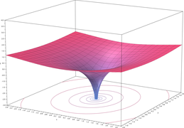
- График натурального логарифма
Определение натурального логарифма
Когда e y = x, натуральный логарифм (ln) числа x выглядит следующим образом:
ln(x) = loge(x) = y
Связь с экспоненциальной функцией
Функция логарифма ln(x) является обратной к экспоненциальной функции ex.
Для х > 0,
f (f -1(x)) = eln(x) = x
или
f -1(f (x)) = ln(ex) = x
Свойства натурального логарифма
| Свойство | Формула | Пример |
| Логарифм умножения | ln (x ⋅ y) = ln (x) + ln (y) | ln (3 ⋅ 7) = ln (3) + ln (7) |
| Логарифм деления | ln (x / y) = ln (x) — ln (y) | ln (3 / 7) = ln (3) — ln (7) |
| Логарифм степени | ln (x y) = y ⋅ ln (x) | ln (28) = 8 ⋅ ln (2) |
| Логарифм корня |  |
 |
| Производная логарифма | f (x) = ln (x) ⇒ f ‘ (x) = 1 / x | |
| Интеграл логарифма | ∫ ln (x) dx = x ⋅ (ln (x) — 1) + C | |
| Логарифм отрицательного числа | ln (x) не определен, если x ≤ 0 | |
| Логарифм числа 0 | ln (0) не определен | |
| Логарифм числа 1 | ln (1) = 0 | |
| Логарифм комплексного числа | log z = ln (r) + i (θ + 2nπ) = ln (√(x 2 + y 2)) + i · arctan (y/x)), для комплексного числа z = re iθ = x + iy |
|
| Логарифм бесконечности | lim ln (x) = ∞, если x → ∞ | |
| Тождество Эйлера | ln (-1) = i ⋅ π |
microexcel.ru
Таблица натуральных логарифмов
| x | ln x |
| 0 | не определен |
| 0+ | — ∞ |
| 0.0001 | -9.210340 |
| 0.001 | -6.907755 |
| 0.01 | -4.605170 |
| 0.1 | -2.302585 |
| 1 | 0 |
| 2 | 0.693147 |
| e ≈ 2.7183 | 1 |
| 3 | 1.098612 |
| 4 | 1.386294 |
| 5 | 1.609438 |
| 6 | 1.791759 |
| 7 | 1.945910 |
| 8 | 2.079442 |
| 9 | 2.197225 |
| 10 | 2.302585 |
| 20 | 2.995732 |
| 30 | 3.401197 |
| 40 | 3.688879 |
| 50 | 3.912023 |
| 60 | 4.094345 |
| 70 | 4.248495 |
| 80 | 4.382027 |
| 90 | 4.499810 |
| 100 | 4.605170 |
| 200 | 5.298317 |
| 300 | 5.703782 |
| 400 | 5.991465 |
| 500 | 6.214608 |
| 600 | 6.396930 |
| 700 | 6.551080 |
| 800 | 6.684612 |
| 900 | 6.802395 |
| 1000 | 6.907755 |
| 10000 | 9.210340 |
График натурального логарифма
Функция натурального логарифма задается как y = ln x. Существует только при неотрицательных значениях переменной x. График выглядит так:

| Natural logarithm | |
|---|---|

Graph of part of the natural logarithm function. The function slowly grows to positive infinity as x increases, and slowly goes to negative infinity as x approaches 0 («slowly» as compared to any power law of x). |
|
| General information | |
| General definition |  |
| Motivation of invention | Analytic proofs |
| Fields of application | Pure and applied mathematics |
| Domain, Codomain and Image | |
| Domain |  |
| Codomain |  |
| Image | |
| Specific values | |
| Value at +∞ | +∞ |
| Value at e | 1 |
| Specific features | |
| Asymptote |  |
| Root | 1 |
| Inverse |  |
| Derivative |  |
| Antiderivative |  |
The natural logarithm of a number is its logarithm to the base of the mathematical constant e, which is an irrational and transcendental number approximately equal to 2.718281828459. The natural logarithm of x is generally written as ln x, loge x, or sometimes, if the base e is implicit, simply log x.[1][2] Parentheses are sometimes added for clarity, giving ln(x), loge(x), or log(x). This is done particularly when the argument to the logarithm is not a single symbol, so as to prevent ambiguity.
The natural logarithm of x is the power to which e would have to be raised to equal x. For example, ln 7.5 is 2.0149…, because e2.0149… = 7.5. The natural logarithm of e itself, ln e, is 1, because e1 = e, while the natural logarithm of 1 is 0, since e0 = 1.
The natural logarithm can be defined for any positive real number a as the area under the curve y = 1/x from 1 to a[3] (with the area being negative when 0 < a < 1). The simplicity of this definition, which is matched in many other formulas involving the natural logarithm, leads to the term «natural». The definition of the natural logarithm can then be extended to give logarithm values for negative numbers and for all non-zero complex numbers, although this leads to a multi-valued function: see Complex logarithm for more.
The natural logarithm function, if considered as a real-valued function of a positive real variable, is the inverse function of the exponential function, leading to the identities:

Like all logarithms, the natural logarithm maps multiplication of positive numbers into addition:
- [4]

Logarithms can be defined for any positive base other than 1, not only e. However, logarithms in other bases differ only by a constant multiplier from the natural logarithm, and can be defined in terms of the latter,  .
.
Logarithms are useful for solving equations in which the unknown appears as the exponent of some other quantity. For example, logarithms are used to solve for the half-life, decay constant, or unknown time in exponential decay problems. They are important in many branches of mathematics and scientific disciplines, and are used to solve problems involving compound interest.
History[edit]
The concept of the natural logarithm was worked out by Gregoire de Saint-Vincent and Alphonse Antonio de Sarasa before 1649.[5] Their work involved quadrature of the hyperbola with equation xy = 1, by determination of the area of hyperbolic sectors. Their solution generated the requisite «hyperbolic logarithm» function, which had the properties now associated with the natural logarithm.
An early mention of the natural logarithm was by Nicholas Mercator in his work Logarithmotechnia, published in 1668,[6] although the mathematics teacher John Speidell had already compiled a table of what in fact were effectively natural logarithms in 1619.[7] It has been said that Speidell’s logarithms were to the base e, but this is not entirely true due to complications with the values being expressed as integers.[7]: 152
Notational conventions[edit]
The notations ln x and loge x both refer unambiguously to the natural logarithm of x, and log x without an explicit base may also refer to the natural logarithm. This usage is common in mathematics, along with some scientific contexts as well as in many programming languages.[nb 1] In some other contexts such as chemistry, however, log x can be used to denote the common (base 10) logarithm. It may also refer to the binary (base 2) logarithm in the context of computer science, particularly in the context of time complexity.
Definitions[edit]
The natural logarithm can be defined in several equivalent ways.
Inverse of exponential[edit]
The most general definition is as the inverse function of  , so that
  . Because is positive and invertible for any real input
  , this definition of
  is well defined for any positive x. For the complex numbers,
  is not invertible, so
  is a multivalued function. In order to make a proper, single-output function, we therefore need to restrict it to a particular principal branch, often denoted by
  . As the inverse function of , can be defined by inverting the usual definition of :

Doing so yields:
![{displaystyle ln(z)=lim _{nto infty }ncdot ({sqrt[{n}]{z}}-1)}](https://wikimedia.org/api/rest_v1/media/math/render/svg/bba681ea4108b1376919349999b5c3ae9bd08e3b)
This definition therefore derives its own principal branch from the principal branch of nth roots.
Integral definition[edit]

ln a as the area of the shaded region under the curve f(x) = 1/x from 1 to a. If a is less than 1, the area taken to be negative.

The area under the hyperbola satisfies the logarithm rule. Here A(s,t) denotes the area under the hyperbola between s and t.
The natural logarithm of a positive, real number a may be defined as the area under the graph of the hyperbola with equation y = 1/x between x = 1 and x = a. This is the integral[3]

If a is less than 1, then this area is considered to be negative.
This function is a logarithm because it satisfies the fundamental multiplicative property of a logarithm:[4]

This can be demonstrated by splitting the integral that defines ln ab into two parts, and then making the variable substitution x = at (so dx = a dt) in the second part, as follows:
![{displaystyle {begin{aligned}ln ab=int _{1}^{ab}{frac {1}{x}},dx&=int _{1}^{a}{frac {1}{x}},dx+int _{a}^{ab}{frac {1}{x}},dx\[5pt]&=int _{1}^{a}{frac {1}{x}},dx+int _{1}^{b}{frac {1}{at}}a,dt\[5pt]&=int _{1}^{a}{frac {1}{x}},dx+int _{1}^{b}{frac {1}{t}},dt\[5pt]&=ln a+ln b.end{aligned}}}](https://wikimedia.org/api/rest_v1/media/math/render/svg/d7210259ed243c3b86451e39eb2b50dccc7832e1)
In elementary terms, this is simply scaling by 1/a in the horizontal direction and by a in the vertical direction. Area does not change under this transformation, but the region between a and ab is reconfigured. Because the function a/(ax) is equal to the function 1/x, the resulting area is precisely ln b.
The number e can then be defined to be the unique real number a such that ln a = 1.
The natural logarithm also has an improper integral representation,[8] which can be derived with Fubini’s theorem as follows:

Properties[edit]
Derivative[edit]
The derivative of the natural logarithm as a real-valued function on the positive reals is given by[3]

How to establish this derivative of the natural logarithm depends on how it is defined firsthand. If the natural logarithm is defined as the integral

then the derivative immediately follows from the first part of the fundamental theorem of calculus.
On the other hand, if the natural logarithm is defined as the inverse of the (natural) exponential function, then the derivative (for x > 0) can be found by using the properties of the logarithm and a definition of the exponential function. From the definition of the number  the exponential function can be defined as
  , where
  The derivative can then be found from first principles.
![{displaystyle {begin{aligned}{frac {d}{dx}}ln x&=lim _{hto 0}{frac {ln(x+h)-ln x}{h}}\&=lim _{hto 0}left[{frac {1}{h}}ln left({frac {x+h}{x}}right)right]\&=lim _{hto 0}left[ln left(left(1+{frac {h}{x}}right)^{frac {1}{h}}right)right]quad &&{text{all above for logarithmic properties}}\&=ln left[lim _{hto 0}left(1+{frac {h}{x}}right)^{frac {1}{h}}right]quad &&{text{for continuity of the logarithm}}\&=ln e^{1/x}quad &&{text{for the definition of }}e^{x}=lim _{hto 0}(1+hx)^{1/h}\&={frac {1}{x}}quad &&{text{for the definition of the ln as inverse function.}}end{aligned}}}](https://wikimedia.org/api/rest_v1/media/math/render/svg/7ac40a28d99ea3c3c0e2fbcfad73461fa5837fa6)
Also, we have:

so, unlike its inverse function  , a constant in the function doesn’t alter the differential.
Series[edit]
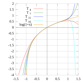
The Taylor polynomials for ln(1 + x) only provide accurate approximations in the range −1 < x ≤ 1. Beyond some x > 1, the Taylor polynomials of higher degree are increasingly worse approximations.
Since the natural logarithm is undefined at 0, itself does not have a Maclaurin series, unlike many other elementary functions. Instead, one looks for Taylor expansions around other points. For example, if  then[9]

This is the Taylor series for ln x around 1. A change of variables yields the Mercator series:

valid for |x| ≤ 1 and x ≠ −1.
Leonhard Euler,[10] disregarding  , nevertheless applied this series to x = −1 to show that the harmonic series equals the natural logarithm of 1/(1 − 1), that is, the logarithm of infinity. Nowadays, more formally, one can prove that the harmonic series truncated at N is close to the logarithm of N, when N is large, with the difference converging to the Euler–Mascheroni constant.
The figure is a graph of ln(1 + x) and some of its Taylor polynomials around 0. These approximations converge to the function only in the region −1 < x ≤ 1; outside this region, the higher-degree Taylor polynomials devolve to worse approximations for the function.
A useful special case for positive integers n, taking  , is:
, is:

If  then
then

Now, taking  for positive integers n, we get:

If  then
then

Since

we arrive at

Using the substitution again for positive integers n, we get:

This is, by far, the fastest converging of the series described here.
The natural logarithm can also be expressed as an infinite product:[11]
![{displaystyle ln(x)=(x-1)prod _{k=1}^{infty }left({frac {2}{1+{sqrt[{2^{k}}]{x}}}}right)}](https://wikimedia.org/api/rest_v1/media/math/render/svg/19a685fc50f560fbfd45cd8c625c839137a0cb42)
Two examples might be:
![{displaystyle ln(2)=left({frac {2}{1+{sqrt {2}}}}right)left({frac {2}{1+{sqrt[{4}]{2}}}}right)left({frac {2}{1+{sqrt[{8}]{2}}}}right)left({frac {2}{1+{sqrt[{16}]{2}}}}right)...}](https://wikimedia.org/api/rest_v1/media/math/render/svg/b7b509b3f7ce72ef554df0dfb48f10dbdc772055)
![{displaystyle pi =(2i+2)left({frac {2}{1+{sqrt {i}}}}right)left({frac {2}{1+{sqrt[{4}]{i}}}}right)left({frac {2}{1+{sqrt[{8}]{i}}}}right)left({frac {2}{1+{sqrt[{16}]{i}}}}right)...}](https://wikimedia.org/api/rest_v1/media/math/render/svg/438561a80d9075271b2dcd15bea94412d2683e69)
From this identity, we can easily get that:

For example:
![{displaystyle {frac {1}{ln(2)}}=2-{frac {sqrt {2}}{2+2{sqrt {2}}}}-{frac {sqrt[{4}]{2}}{4+4{sqrt[{4}]{2}}}}-{frac {sqrt[{8}]{2}}{8+8{sqrt[{8}]{2}}}}cdots }](https://wikimedia.org/api/rest_v1/media/math/render/svg/def29e93c87165f8547949c7e10896c45dc22d2f)
The natural logarithm in integration[edit]
The natural logarithm allows simple integration of functions of the form g(x) = f ‘(x)/f(x): an antiderivative of g(x) is given by ln(|f(x)|). This is the case because of the chain rule and the following fact:

In other words, when integrating over an interval of the real line that does not include then

where C is an arbitrary constant of integration.[12]
Likewise, when the integral is over an interval where  ,
,

For example, consider the integral of tan(x) over an interval that does not include points where tan(x) is infinite:

The natural logarithm can be integrated using integration by parts:

Let:


then:

Efficient computation[edit]
For ln(x) where x > 1, the closer the value of x is to 1, the faster the rate of convergence of its Taylor series centered at 1. The identities associated with the logarithm can be leveraged to exploit this:

Such techniques were used before calculators, by referring to numerical tables and performing manipulations such as those above.
Natural logarithm of 10[edit]
The natural logarithm of 10, which has the decimal expansion 2.30258509…,[13] plays a role for example in the computation of natural logarithms of numbers represented in scientific notation, as a mantissa multiplied by a power of 10:

This means that one can effectively calculate the logarithms of numbers with very large or very small magnitude using the logarithms of a relatively small set of decimals in the range [1, 10).
High precision[edit]
To compute the natural logarithm with many digits of precision, the Taylor series approach is not efficient since the convergence is slow. Especially if x is near 1, a good alternative is to use Halley’s method or Newton’s method to invert the exponential function, because the series of the exponential function converges more quickly. For finding the value of y to give exp(y) − x = 0 using Halley’s method, or equivalently to give exp(y/2) − x exp(−y/2) = 0 using Newton’s method, the iteration simplifies to

which has cubic convergence to ln(x).
Another alternative for extremely high precision calculation is the formula[14][15]

where M denotes the arithmetic-geometric mean of 1 and 4/s, and

with m chosen so that p bits of precision is attained. (For most purposes, the value of 8 for m is sufficient.) In fact, if this method is used, Newton inversion of the natural logarithm may conversely be used to calculate the exponential function efficiently. (The constants ln 2 and π can be pre-computed to the desired precision using any of several known quickly converging series.) Or, the following formula can be used:

where

are the Jacobi theta functions.[16]
Based on a proposal by William Kahan and first implemented in the Hewlett-Packard HP-41C calculator in 1979 (referred to under «LN1» in the display, only), some calculators, operating systems (for example Berkeley UNIX 4.3BSD[17]), computer algebra systems and programming languages (for example C99[18]) provide a special natural logarithm plus 1 function, alternatively named LNP1,[19][20] or log1p[18] to give more accurate results for logarithms close to zero by passing arguments x, also close to zero, to a function log1p(x), which returns the value ln(1+x), instead of passing a value y close to 1 to a function returning ln(y).[18][19][20] The function log1p avoids in the floating point arithmetic a near cancelling of the absolute term 1 with the second term from the Taylor expansion of the ln. This keeps the argument, the result, and intermediate steps all close to zero where they can be most accurately represented as floating-point numbers.[19][20]
In addition to base e the IEEE 754-2008 standard defines similar logarithmic functions near 1 for binary and decimal logarithms: log2(1 + x) and log10(1 + x).
Similar inverse functions named «expm1»,[18] «expm»[19][20] or «exp1m» exist as well, all with the meaning of expm1(x) = exp(x) − 1.[nb 2]
An identity in terms of the inverse hyperbolic tangent,

gives a high precision value for small values of x on systems that do not implement log1p(x).
Computational complexity[edit]
The computational complexity of computing the natural logarithm using the arithmetic-geometric mean (for both of the above methods) is O(M(n) ln n). Here n is the number of digits of precision at which the natural logarithm is to be evaluated and M(n) is the computational complexity of multiplying two n-digit numbers.
Continued fractions[edit]
While no simple continued fractions are available, several generalized continued fractions are, including:
![{displaystyle {begin{aligned}ln(1+x)&={frac {x^{1}}{1}}-{frac {x^{2}}{2}}+{frac {x^{3}}{3}}-{frac {x^{4}}{4}}+{frac {x^{5}}{5}}-cdots \[5pt]&={cfrac {x}{1-0x+{cfrac {1^{2}x}{2-1x+{cfrac {2^{2}x}{3-2x+{cfrac {3^{2}x}{4-3x+{cfrac {4^{2}x}{5-4x+ddots }}}}}}}}}}end{aligned}}}](https://wikimedia.org/api/rest_v1/media/math/render/svg/92f9f9bda019d60b5ac5d5fd29ea2dd952c5b90a)
![{displaystyle {begin{aligned}ln left(1+{frac {x}{y}}right)&={cfrac {x}{y+{cfrac {1x}{2+{cfrac {1x}{3y+{cfrac {2x}{2+{cfrac {2x}{5y+{cfrac {3x}{2+ddots }}}}}}}}}}}}\[5pt]&={cfrac {2x}{2y+x-{cfrac {(1x)^{2}}{3(2y+x)-{cfrac {(2x)^{2}}{5(2y+x)-{cfrac {(3x)^{2}}{7(2y+x)-ddots }}}}}}}}end{aligned}}}](https://wikimedia.org/api/rest_v1/media/math/render/svg/90abfa2132828fc8eea5d3551dfa4df25dbdfa87)
These continued fractions—particularly the last—converge rapidly for values close to 1. However, the natural logarithms of much larger numbers can easily be computed, by repeatedly adding those of smaller numbers, with similarly rapid convergence.
For example, since 2 = 1.253 × 1.024, the natural logarithm of 2 can be computed as:
![{displaystyle {begin{aligned}ln 2&=3ln left(1+{frac {1}{4}}right)+ln left(1+{frac {3}{125}}right)\[8pt]&={cfrac {6}{9-{cfrac {1^{2}}{27-{cfrac {2^{2}}{45-{cfrac {3^{2}}{63-ddots }}}}}}}}+{cfrac {6}{253-{cfrac {3^{2}}{759-{cfrac {6^{2}}{1265-{cfrac {9^{2}}{1771-ddots }}}}}}}}.end{aligned}}}](https://wikimedia.org/api/rest_v1/media/math/render/svg/bc10de9595aca079ef56e7b76a2a23af56e453da)
Furthermore, since 10 = 1.2510 × 1.0243, even the natural logarithm of 10 can be computed similarly as:
![{displaystyle {begin{aligned}ln 10&=10ln left(1+{frac {1}{4}}right)+3ln left(1+{frac {3}{125}}right)\[10pt]&={cfrac {20}{9-{cfrac {1^{2}}{27-{cfrac {2^{2}}{45-{cfrac {3^{2}}{63-ddots }}}}}}}}+{cfrac {18}{253-{cfrac {3^{2}}{759-{cfrac {6^{2}}{1265-{cfrac {9^{2}}{1771-ddots }}}}}}}}.end{aligned}}}](https://wikimedia.org/api/rest_v1/media/math/render/svg/931b5e1a786450547bd77e466677d9a983974886)
The reciprocal of the natural logarithm can be also written in this way:

For example:

Complex logarithms[edit]
The exponential function can be extended to a function which gives a complex number as ez for any arbitrary complex number z; simply use the infinite series with x=z complex. This exponential function can be inverted to form a complex logarithm that exhibits most of the properties of the ordinary logarithm. There are two difficulties involved: no x has ex = 0; and it turns out that e2iπ = 1 = e0. Since the multiplicative property still works for the complex exponential function, ez = ez+2kiπ, for all complex z and integers k.
So the logarithm cannot be defined for the whole complex plane, and even then it is multi-valued—any complex logarithm can be changed into an «equivalent» logarithm by adding any integer multiple of 2iπ at will. The complex logarithm can only be single-valued on the cut plane. For example, ln i = iπ/2 or 5iπ/2 or —3iπ/2, etc.; and although i4 = 1, 4 ln i can be defined as 2iπ, or 10iπ or −6iπ, and so on.
- Plots of the natural logarithm function on the complex plane (principal branch)
-

z = Re(ln(x + yi))
-

z = |(Im(ln(x + yi)))|
-

z = |(ln(x + yi))|
-

Superposition of the previous three graphs


See also[edit]
- Approximating natural exponents (log base e)
- Iterated logarithm
- Napierian logarithm
- List of logarithmic identities
- Logarithm of a matrix
- Logarithmic differentiation
- Logarithmic integral function
- Nicholas Mercator – first to use the term natural logarithm
- Polylogarithm
- Von Mangoldt function
Notes[edit]
- ^ Including C, C++, SAS, MATLAB, Mathematica, Fortran, and some BASIC dialects
- ^ For a similar approach to reduce round-off errors of calculations for certain input values see trigonometric functions like versine, vercosine, coversine, covercosine, haversine, havercosine, hacoversine, hacovercosine, exsecant and excosecant.
References[edit]
- ^ G.H. Hardy and E.M. Wright, An Introduction to the Theory of Numbers, 4th Ed., Oxford 1975, footnote to paragraph 1.7: «log x is, of course, the ‘Naperian’ logarithm of x, to base e. ‘Common’ logarithms have no mathematical interest«.
- ^ Mortimer, Robert G. (2005). Mathematics for physical chemistry (3rd ed.). Academic Press. p. 9. ISBN 0-12-508347-5. Extract of page 9
- ^ a b c Weisstein, Eric W. «Natural Logarithm». mathworld.wolfram.com. Retrieved 2020-08-29.
- ^ a b «Rules, Examples, & Formulas». Logarithm. Encyclopedia Britannica. Retrieved 2020-08-29.
- ^ Burn, R.P. (2001). Alphonse Antonio de Sarasa and Logarithms. Historia Mathematica. pp. 28:1–17.
- ^ O’Connor, J. J.; Robertson, E. F. (September 2001). «The number e». The MacTutor History of Mathematics archive. Retrieved 2009-02-02.
- ^ a b Cajori, Florian (1991). A History of Mathematics (5th ed.). AMS Bookstore. p. 152. ISBN 0-8218-2102-4.
- ^ An improper integral representation of the natural logarithm., retrieved 2022-09-24
- ^ ««Logarithmic Expansions» at Math2.org».
- ^ Leonhard Euler, Introductio in Analysin Infinitorum. Tomus Primus. Bousquet, Lausanne 1748. Exemplum 1, p. 228; quoque in: Opera Omnia, Series Prima, Opera Mathematica, Volumen Octavum, Teubner 1922
- ^ RUFFA, Anthony. «A PROCEDURE FOR GENERATING INFINITE SERIES IDENTITIES» (PDF). International Journal of Mathematics and Mathematical Sciences. International Journal of Mathematics and Mathematical Sciences. Retrieved 2022-02-27. (Page 3654, equation 2.6)
- ^ For a detailed proof see for instance: George B. Thomas, Jr and Ross L. Finney, Calculus and Analytic Geometry, 5th edition, Addison-Wesley 1979, Section 6-5 pages 305-306.
- ^ OEIS: A002392
- ^ Sasaki, T.; Kanada, Y. (1982). «Practically fast multiple-precision evaluation of log(x)». Journal of Information Processing. 5 (4): 247–250. Retrieved 2011-03-30.
- ^ Ahrendt, Timm (1999). «Fast Computations of the Exponential Function». Stacs 99. Lecture Notes in Computer Science. 1564: 302–312. doi:10.1007/3-540-49116-3_28. ISBN 978-3-540-65691-3.
- ^ Borwein, Jonathan M.; Borwein, Peter B. (1987). Pi and the AGM: A Study in Analytic Number Theory and Computational Complexity (First ed.). Wiley-Interscience. ISBN 0-471-83138-7. page 225
- ^ Beebe, Nelson H. F. (2017-08-22). «Chapter 10.4. Logarithm near one». The Mathematical-Function Computation Handbook — Programming Using the MathCW Portable Software Library (1 ed.). Salt Lake City, UT, USA: Springer International Publishing AG. pp. 290–292. doi:10.1007/978-3-319-64110-2. ISBN 978-3-319-64109-6. LCCN 2017947446. S2CID 30244721.
In 1987, Berkeley UNIX 4.3BSD introduced the log1p() function
- ^ a b c d Beebe, Nelson H. F. (2002-07-09). «Computation of expm1 = exp(x)−1» (PDF). 1.00. Salt Lake City, Utah, USA: Department of Mathematics, Center for Scientific Computing, University of Utah. Retrieved 2015-11-02.
- ^ a b c d HP 48G Series – Advanced User’s Reference Manual (AUR) (4 ed.). Hewlett-Packard. December 1994 [1993]. HP 00048-90136, 0-88698-01574-2. Retrieved 2015-09-06.
- ^ a b c d HP 50g / 49g+ / 48gII graphing calculator advanced user’s reference manual (AUR) (2 ed.). Hewlett-Packard. 2009-07-14 [2005]. HP F2228-90010. Retrieved 2015-10-10. Searchable PDF
Калькулятор натуральных логарифмов поможет найти логарифм по основанию e, где e — иррациональная константа, равная приблизительно 2,72.
Обозначение натурального логарифма
Для обозначения натурального логарифма существует несколько способов:
- ln
- loge
Так же возможно написание прописными буквами.
Что такое натуральный логарифм
Натуральный логарифм
Понятие натурального логарифма лучше проиллюстрировать примером. Например, натуральный логарифм числа 2 равен 0,693147180 потому, что
e0,693147180 = 2
Здесь e — основание натурального логарифма.
e =2,718281828
Таким образом натуральный логарифм — это степень, в которую нужно возвести число e для получения исходного числа, логарифм которого мы ищем. Вычисление натурального логарифма несложная задача и наш калькулятор поможет с расчетом.
Натуральный логарифм нуля не существует. Для чисел меньше единицы натуральный логарифм отрицательный.
Таблица натуральных логарифмов некоторых чисел
| x | ln x |
| 1 | 0 |
| 2 | 0,693147 |
| 3 | 1,098612 |
| 4 | 1,386294 |
| 5 | 1,609438 |
| 6 | 1,791759 |
| 7 | 1,94591 |
| 8 | 2,079442 |
| 9 | 2,197225 |
| 10 | 2,302585 |
| 100 | 4,60517 |
| 1000 | 6,907755 |
| 10000 | 9,21034 |
| 100000 | 11,51293 |
Ваша оценка
[Оценок: 285 Средняя: 2.8]
Калькулятор натуральных логарифмов Автор admin средний рейтинг 2.8/5 — 285 рейтинги пользователей
Краткая история логарифма
Логарифм имеет много применений в науке и инженерии.
Естественный логарифм имеет констант в своем основании, его использование широко распространено в дискретной математике, особенно в исчислении. Двоичный логарифм использует базу и занимает видное место в информатике. Логарифмы были введены Джоном Нейпиром в начале XVII века, как средство упрощения расчетов. Они были легко приняты учеными, инженерами и другими, чтобы облегчать вычисления. Современное понятие логарифмов исходит от Леонарда Эйлера, который связал их с экспоненциальной функцией в XVIII веке
Определение логарифма
Логарифмы — это показатель степени: в какую степень надо возвести число, которое стоит в основании, чтобы получить число в выражении логарифма. Например, (log_28 ) в какую степень надо возвести (2), чтобы получить (8) это (log_28 =3).
Читается, как логарифм (8) по основанию (2) равен (3).
Определение логарифма:
(log_ax=b) (x=a^b)
Очень важно помнить, где находится аргумент, а где основание
Если (x=1), то (b) равен (o), так как ненулевое число в нулевой степени всегда равно единице (x^0=1), (x) не равно (0).
Некоторые логарифмы в результате получают иррациональное число, пример (log_310) результат будет лежать на промежутке: (3^2 < 10< 3^3.)
ОДЗ логарифма
ОДЗ (область допустимых значений) логарифма – это множество всех действительных чисел, для которых определена данная функция. Для логарифмической функции с основанием a ОДЗ определяется следующим образом:
x > 0 (если a > 1) или x < 0 (если 0 < a < 1)
То есть аргумент логарифма должен быть положительным, если основание больше 1, и отрицательным, если основание меньше 1.
Область допустимых значений логарифма — главное:
- Аргумент и основание не могут быть равны нулю и отрицательными числами.
- Основание не может быть равно единице, поскольку единица в любой степени все равно остается единицей.
- Число b может быть любым.
- ОДЗ логарифма (log_a x = b ⇒ x > 0, a > 0, a ≠ 1).
Виды логарифмов
Существует два основных вида логарифмов: обычные (или десятичные) логарифмы и натуральные логарифмы.
- Обычный (десятичный) логарифм (log base 10): логарифм, основание которого равно 10. Обычный логарифм числа y обозначается как log(y) или lg(y) и определяется формулой:
log(y) = x, если 10^x = y
Например, log(100) = 2, так как 10^2 = 100.
- Натуральный логарифм (log base e): логарифм, основание которого равно числу e (приблизительно 2,71828). Натуральный логарифм числа y обозначается как ln(y) и определяется формулой:
ln(y) = x, если e^x = y
Например, ln(e) = 1, так как e^1 = e.
Обычные и натуральные логарифмы связаны друг с другом формулой:
log(y) = ln(y) / ln(10)
где ln(10) ≈ 2,3026.
Существуют также логарифмы с другими основаниями (например, логарифм по основанию 2), но они реже используются в практических расчетах.
Десятичные логарифмы
Десятичные логарифмы – логарифмы, в основании которых стоит (10). Пример (log_{10}10 =1),
Log10100 =2. Записывают их в виде (lg 10 = 1), (lg 100 = 2.)
Натуральный логарифм
Натуральный логарифм – логарифм, в основании которого стоит (e). Что означает (e)? Это иррациональное число, бесконечное непериодическое десятичное число, математическая константа, которую надо запомнить:
(e = 2,718281828459…)
(ln x = log_e x)
Часто задаваемые вопросы
✅ Как часто проходят занятия?
↪ Мы предлагаем индивидуальный график занятий, который учитывает ваше расписание и потребности ребенка. Обычно занятия проходят один или два раза в неделю.
✅ Какие материалы будут использоваться на занятиях?
↪ Мы используем разнообразные материалы, такие как учебники, аудио и видео материалы, игры и тесты. Все материалы выбираются исходя из возраста и уровня владения языком ученика.
✅ Как проходят занятия?
↪ Наши занятия проводятся онлайн с помощью специальных программ для видео-конференций. Репетитор будет работать с вашим ребенком индивидуально. Мы стремимся сделать наши занятия интерактивными, увлекательными и полезными.
Больше уроков и заданий по всем школьным предметам в онлайн-школе «Альфа». Запишитесь на пробное занятие прямо сейчас!
Запишитесь на бесплатное тестирование знаний!