This article is about the term used in probability theory and statistics. For other uses, see Expected value (disambiguation).
«E(X)» redirects here. For the  function, see Exponential function.
In probability theory, the expected value (also called expectation, expectancy, mathematical expectation, mean, average, or first moment) is a generalization of the weighted average. Informally, the expected value is the arithmetic mean of a large number of independently selected outcomes of a random variable.
The expected value of a random variable with a finite number of outcomes is a weighted average of all possible outcomes. In the case of a continuum of possible outcomes, the expectation is defined by integration. In the axiomatic foundation for probability provided by measure theory, the expectation is given by Lebesgue integration.
The expected value of a random variable X is often denoted by E(X), E[X], or EX, with E also often stylized as E or  [1][2][3]
History[edit]
The idea of the expected value originated in the middle of the 17th century from the study of the so-called problem of points, which seeks to divide the stakes in a fair way between two players, who have to end their game before it is properly finished.[4] This problem had been debated for centuries. Many conflicting proposals and solutions had been suggested over the years when it was posed to Blaise Pascal by French writer and amateur mathematician Chevalier de Méré in 1654. Méré claimed that this problem couldn’t be solved and that it showed just how flawed mathematics was when it came to its application to the real world. Pascal, being a mathematician, was provoked and determined to solve the problem once and for all.
He began to discuss the problem in the famous series of letters to Pierre de Fermat. Soon enough, they both independently came up with a solution. They solved the problem in different computational ways, but their results were identical because their computations were based on the same fundamental principle. The principle is that the value of a future gain should be directly proportional to the chance of getting it. This principle seemed to have come naturally to both of them. They were very pleased by the fact that they had found essentially the same solution, and this in turn made them absolutely convinced that they had solved the problem conclusively; however, they did not publish their findings. They only informed a small circle of mutual scientific friends in Paris about it.[5]
In Dutch mathematician Christiaan Huygens’ book, he considered the problem of points, and presented a solution based on the same principle as the solutions of Pascal and Fermat. Huygens published his treatise in 1657, (see Huygens (1657)) «De ratiociniis in ludo aleæ» on probability theory just after visiting Paris. The book extended the concept of expectation by adding rules for how to calculate expectations in more complicated situations than the original problem (e.g., for three or more players), and can be seen as the first successful attempt at laying down the foundations of the theory of probability.
In the foreword to his treatise, Huygens wrote:
It should be said, also, that for some time some of the best mathematicians of France have occupied themselves with this kind of calculus so that no one should attribute to me the honour of the first invention. This does not belong to me. But these savants, although they put each other to the test by proposing to each other many questions difficult to solve, have hidden their methods. I have had therefore to examine and go deeply for myself into this matter by beginning with the elements, and it is impossible for me for this reason to affirm that I have even started from the same principle. But finally I have found that my answers in many cases do not differ from theirs.
— Edwards (2002)
During his visit to France in 1655, Huygens learned about de Méré’s Problem. From his correspondence with Carcavine a year later (in 1656), he realized his method was essentially the same as Pascal’s. Therefore, he knew about Pascal’s priority in this subject before his book went to press in 1657.[6]
In the mid-nineteenth century, Pafnuty Chebyshev became the first person to think systematically in terms of the expectations of random variables.[7]
Etymology[edit]
Neither Pascal nor Huygens used the term «expectation» in its modern sense. In particular, Huygens writes:[8]
That any one Chance or Expectation to win any thing is worth just such a Sum, as wou’d procure in the same Chance and Expectation at a fair Lay. … If I expect a or b, and have an equal chance of gaining them, my Expectation is worth (a+b)/2.
More than a hundred years later, in 1814, Pierre-Simon Laplace published his tract «Théorie analytique des probabilités«, where the concept of expected value was defined explicitly:[9]
… this advantage in the theory of chance is the product of the sum hoped for by the probability of obtaining it; it is the partial sum which ought to result when we do not wish to run the risks of the event in supposing that the division is made proportional to the probabilities. This division is the only equitable one when all strange circumstances are eliminated; because an equal degree of probability gives an equal right for the sum hoped for. We will call this advantage mathematical hope.
Notations[edit]
The use of the letter E to denote expected value goes back to W. A. Whitworth in 1901.[10] The symbol has become popular since then for English writers. In German, E stands for «Erwartungswert», in Spanish for «Esperanza matemática», and in French for «Espérance mathématique».[11]
When «E» is used to denote expected value, authors use a variety of stylization: the expectation operator can be stylized as E (upright), E (italic), or  (in blackboard bold), while a variety of bracket notations (such as E(X), E[X], and EX) are all used.
Another popular notation is μX, whereas ⟨X⟩, ⟨X⟩av, and  are commonly used in physics,[12] and M(X) in Russian-language literature.
Definition[edit]
As discussed above, there are several context-dependent ways of defining the expected value. The simplest and original definition deals with the case of finitely many possible outcomes, such as in the flip of a coin. With the theory of infinite series, this can be extended to the case of countably many possible outcomes. It is also very common to consider the distinct case of random variables dictated by (piecewise-)continuous probability density functions, as these arise in many natural contexts. All of these specific definitions may be viewed as special cases of the general definition based upon the mathematical tools of measure theory and Lebesgue integration, which provide these different contexts with an axiomatic foundation and common language.
Any definition of expected value may be extended to define an expected value of a multidimensional random variable, i.e. a random vector X. It is defined component by component, as E[X]i = E[Xi]. Similarly, one may define the expected value of a random matrix X with components Xij by E[X]ij = E[Xij].
Random variables with finitely many outcomes[edit]
Consider a random variable X with a finite list x1, …, xk of possible outcomes, each of which (respectively) has probability p1, …, pk of occurring. The expectation of X is defined as[13]
![{displaystyle operatorname {E} [X]=x_{1}p_{1}+x_{2}p_{2}+cdots +x_{k}p_{k}.}](https://wikimedia.org/api/rest_v1/media/math/render/svg/77f1b12ae3ea9d1b9e872c95173ba2dfe4476253)
Since the probabilities must satisfy p1 + ⋅⋅⋅ + pk = 1, it is natural to interpret E[X] as a weighted average of the xi values, with weights given by their probabilities pi.
In the special case that all possible outcomes are equiprobable (that is, p1 = ⋅⋅⋅ = pk), the weighted average is given by the standard average. In the general case, the expected value takes into account the fact that some outcomes are more likely than others.
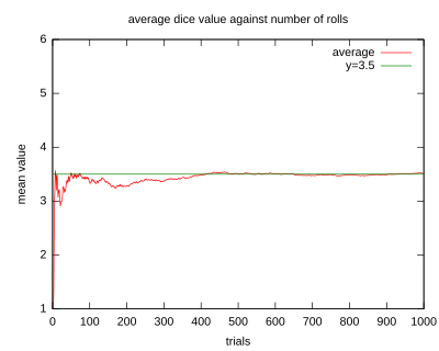
An illustration of the convergence of sequence averages of rolls of a die to the expected value of 3.5 as the number of rolls (trials) grows.
Examples[edit]
![{displaystyle operatorname {E} [X]=1cdot {frac {1}{6}}+2cdot {frac {1}{6}}+3cdot {frac {1}{6}}+4cdot {frac {1}{6}}+5cdot {frac {1}{6}}+6cdot {frac {1}{6}}=3.5.}](https://wikimedia.org/api/rest_v1/media/math/render/svg/d535e1c37fd63db36fd0878e39b43ea7fa513ea4)
- If one rolls the die
 times and computes the average (arithmetic mean) of the results, then as grows, the average will almost surely converge to the expected value, a fact known as the strong law of large numbers.
- The roulette game consists of a small ball and a wheel with 38 numbered pockets around the edge. As the wheel is spun, the ball bounces around randomly until it settles down in one of the pockets. Suppose random variable represents the (monetary) outcome of a $1 bet on a single number («straight up» bet). If the bet wins (which happens with probability 1/38 in American roulette), the payoff is $35; otherwise the player loses the bet. The expected profit from such a bet will be
![{displaystyle operatorname {E} [,{text{gain from }}$1{text{ bet}},]=-$1cdot {frac {37}{38}}+$35cdot {frac {1}{38}}=-${frac {1}{19}}.}](https://wikimedia.org/api/rest_v1/media/math/render/svg/efa6df424d69a14b24a7b598b5e0f1e6e426bff1)
- That is, the expected value to be won from a $1 bet is −$1/19. Thus, in 190 bets, the net loss will probably be about $10.
Random variables with countably many outcomes[edit]
Informally, the expectation of a random variable with a countable set of possible outcomes is defined analogously as the weighted average of all possible outcomes, where the weights are given by the probabilities of realizing each given value. This is to say that
![operatorname {E} [X]=sum _{i=1}^{infty }x_{i},p_{i},](https://wikimedia.org/api/rest_v1/media/math/render/svg/ef6f4efe003752f5353cfb1ed00235f374455805)
where x1, x2, … are the possible outcomes of the random variable X and p1, p2, … are their corresponding probabilities. In many non-mathematical textbooks, this is presented as the full definition of expected values in this context.[14]
However, there are some subtleties with infinite summation, so the above formula is not suitable as a mathematical definition. In particular, the Riemann series theorem of mathematical analysis illustrates that the value of certain infinite sums involving positive and negative summands depends on the order in which the summands are given. Since the outcomes of a random variable have no naturally given order, this creates a difficulty in defining expected value precisely.
For this reason, many mathematical textbooks only consider the case that the infinite sum given above converges absolutely, which implies that the infinite sum is a finite number independent of the ordering of summands.[15] In the alternative case that the infinite sum does not converge absolutely, one says the random variable does not have finite expectation.[15]
Examples[edit]
Random variables with density[edit]
Now consider a random variable X which has a probability density function given by a function f on the real number line. This means that the probability of X taking on a value in any given open interval is given by the integral of f over that interval. The expectation of X is then given by the integral[16]
![{displaystyle operatorname {E} [X]=int _{-infty }^{infty }xf(x),dx.}](https://wikimedia.org/api/rest_v1/media/math/render/svg/78baa8f12272973778deb275cdbb6a624acb0dc2)
A general and mathematically precise formulation of this definition uses measure theory and Lebesgue integration, and the corresponding theory of absolutely continuous random variables is described in the next section. The density functions of many common distributions are piecewise continuous, and as such the theory is often developed in this restricted setting.[17] For such functions, it is sufficient to only consider the standard Riemann integration. Sometimes continuous random variables are defined as those corresponding to this special class of densities, although the term is used differently by various authors.
Analogously to the countably-infinite case above, there are subtleties with this expression due to the infinite region of integration. Such subtleties can be seen concretely if the distribution of X is given by the Cauchy distribution Cauchy(0, π), so that f(x) = (x2 + π2)−1. It is straightforward to compute in this case that

The limit of this expression as a → −∞ and b → ∞ does not exist: if the limits are taken so that a = −b, then the limit is zero, while if the constraint 2a = −b is taken, then the limit is ln(2).
To avoid such ambiguities, in mathematical textbooks it is common to require that the given integral converges absolutely, with E[X] left undefined otherwise.[18] However, measure-theoretic notions as given below can be used to give a systematic definition of E[X] for more general random variables X.
Arbitrary real-valued random variables[edit]
All definitions of the expected value may be expressed in the language of measure theory. In general, if X is a real-valued random variable defined on a probability space (Ω, Σ, P), then the expected value of X, denoted by E[X], is defined as the Lebesgue integral[19]
![{displaystyle operatorname {E} [X]=int _{Omega }X,doperatorname {P} .}](https://wikimedia.org/api/rest_v1/media/math/render/svg/d43b61b393c5d8afddd331ac2b9a99e8fb0bac37)
Despite the newly abstract situation, this definition is extremely similar in nature to the very simplest definition of expected values, given above, as certain weighted averages. This is because, in measure theory, the value of the Lebesgue integral of X is defined via weighted averages of approximations of X which take on finitely many values.[20] Moreover, if given a random variable with finitely or countably many possible values, the Lebesgue theory of expectation is identical with the summation formulas given above. However, the Lebesgue theory clarifies the scope of the theory of probability density functions. A random variable X is said to be absolutely continuous if any of the following conditions are satisfied:
- there is a nonnegative measurable function f on the real line such that
-
- for any Borel set A, in which the integral is Lebesgue.

- the cumulative distribution function of X is absolutely continuous.
- for any Borel set A of real numbers with Lebesgue measure equal to zero, the probability of X being valued in A is also equal to zero
- for any positive number ε there is a positive number δ such that: if A is a Borel set with Lebesgue measure less than δ, then the probability of X being valued in A is less than ε.
These conditions are all equivalent, although this is nontrivial to establish.[21] In this definition, f is called the probability density function of X (relative to Lebesgue measure). According to the change-of-variables formula for Lebesgue integration,[22] combined with the law of the unconscious statistician,[23] it follows that
![{displaystyle operatorname {E} [X]equiv int _{Omega }X,doperatorname {P} =int _{mathbb {R} }xf(x),dx}](https://wikimedia.org/api/rest_v1/media/math/render/svg/a482fe9cd2b681480220cea55287286c408a7412)
for any absolutely continuous random variable X. The above discussion of continuous random variables is thus a special case of the general Lebesgue theory, due to the fact that every piecewise-continuous function is measurable.
Infinite expected values[edit]
Expected values as defined above are automatically finite numbers. However, in many cases it is fundamental to be able to consider expected values of ±∞. This is intuitive, for example, in the case of the St. Petersburg paradox, in which one considers a random variable with possible outcomes xi = 2i, with associated probabilities pi = 2−i, for i ranging over all positive integers. According to the summation formula in the case of random variables with countably many outcomes, one has
![{displaystyle operatorname {E} [X]=sum _{i=1}^{infty }x_{i},p_{i}=2cdot {frac {1}{2}}+4cdot {frac {1}{4}}+8cdot {frac {1}{8}}+16cdot {frac {1}{16}}+cdots =1+1+1+1+cdots .}](https://wikimedia.org/api/rest_v1/media/math/render/svg/e5f800b3f19fb7c49f816ed4c13782ae8fc2fdc6)
It is natural to say that the expected value equals +∞.
There is a rigorous mathematical theory underlying such ideas, which is often taken as part of the definition of the Lebesgue integral.[20] The first fundamental observation is that, whichever of the above definitions are followed, any nonnegative random variable whatsoever can be given an unambiguous expected value; whenever absolute convergence fails, then the expected value can be defined as +∞. The second fundamental observation is that any random variable can be written as the difference of two nonnegative random variables. Given a random variable X, one defines the positive and negative parts by X + = max(X, 0) and X − = −min(X, 0). These are nonnegative random variables, and it can be directly checked that X = X + − X −. Since E[X +] and E[X −] are both then defined as either nonnegative numbers or +∞, it is then natural to define:
![{displaystyle operatorname {E} [X]={begin{cases}operatorname {E} [X^{+}]-operatorname {E} [X^{-}]&{text{if }}operatorname {E} [X^{+}]<infty {text{ and }}operatorname {E} [X^{-}]<infty ;\+infty &{text{if }}operatorname {E} [X^{+}]=infty {text{ and }}operatorname {E} [X^{-}]<infty ;\-infty &{text{if }}operatorname {E} [X^{+}]<infty {text{ and }}operatorname {E} [X^{-}]=infty ;\{text{undefined}}&{text{if }}operatorname {E} [X^{+}]=infty {text{ and }}operatorname {E} [X^{-}]=infty .end{cases}}}](https://wikimedia.org/api/rest_v1/media/math/render/svg/d5cf312bcec89a7df3b6580751d6c93ad4248bf8)
According to this definition, E[X] exists and is finite if and only if E[X +] and E[X −] are both finite. Due to the formula |X| = X + + X −, this is the case if and only if E|X| is finite, and this is equivalent to the absolute convergence conditions in the definitions above. As such, the present considerations do not define finite expected values in any cases not previously considered; they are only useful for infinite expectations.
- In the case of the St. Petersburg paradox, one has X − = 0 and so E[X] = +∞ as desired.
- Suppose the random variable X takes values 1, −2,3, −4, … with respective probabilities 6π−2, 6(2π)−2, 6(3π)−2, 6(4π)−2, …. Then it follows that X + takes value 2k−1 with probability 6((2k−1)π)−2 for each positive integer k, and takes value 0 with remaining probability. Similarly, X − takes value 2k with probability 6(2kπ)−2 for each positive integer k and takes value 0 with remaining probability. Using the definition for non-negative random variables, one can show that both E[X +] = ∞ and E[X −] = ∞ (see Harmonic series). Hence, in this case the expectation of X is undefined.
- Similarly, the Cauchy distribution, as discussed above, has undefined expectation.
Expected values of common distributions[edit]
The following table gives the expected values of some commonly occurring probability distributions. The third column gives the expected values both in the form immediately given by the definition, as well as in the simplified form obtained by computation therefrom. The details of these computations, which are not always straightforward, can be found in the indicated references.
| Distribution | Notation | Mean E(X) |
|---|---|---|
| Bernoulli[24] | 
|

|
| Binomial[25] | 
|

|
| Poisson[26] | 
|

|
| Geometric[27] | 
|

|
| Uniform[28] | 
|

|
| Exponential[29] | 
|

|
| Normal[30] | 
|

|
| Standard Normal[31] | 
|

|
| Pareto[32] | 
|

|
| Cauchy[33] | 
|
 is undefined is undefined
|
Properties[edit]
The basic properties below (and their names in bold) replicate or follow immediately from those of Lebesgue integral. Note that the letters «a.s.» stand for «almost surely»—a central property of the Lebesgue integral. Basically, one says that an inequality like  is true almost surely, when the probability measure attributes zero-mass to the complementary event
  .
.
- whenever the right-hand side is well-defined. By induction, this means that the expected value of the sum of any finite number of random variables is the sum of the expected values of the individual random variables, and the expected value scales linearly with a multiplicative constant. Symbolically, for random variables and constants , we have . If we think of the set of random variables with finite expected value as forming a vector space, then the linearity of expectation implies that the expected value is a linear form on this vector space.


![{textstyle operatorname {E} left[sum _{i=1}^{N}a_{i}X_{i}right]=sum _{i=1}^{N}a_{i}operatorname {E} [X_{i}]}](https://wikimedia.org/api/rest_v1/media/math/render/svg/7aa54b6cb62df69950588226116bdeadec16dd85)
- Monotonicity: If (a.s.), and both and exist, then . Proof follows from the linearity and the non-negativity property for , since (a.s.).
- Non-degeneracy: If , then (a.s.).
- If (a.s.), then . In other words, if X and Y are random variables that take different values with probability zero, then the expectation of X will equal the expectation of Y.
- If (a.s.) for some real number c, then . In particular, for a random variable with well-defined expectation, . A well defined expectation implies that there is one number, or rather, one constant that defines the expected value. Thus follows that the expectation of this constant is just the original expected value.
- As a consequence of the formula |X| = X + + X − as discussed above, together with the triangle inequality, it follows that for any random variable with well-defined expectation, one has .
- Let 1A denote the indicator function of an event A, then E[1A] is given by the probability of A. This is nothing but a different way of stating the expectation of a Bernoulli random variable, as calculated in the table above.
- Formulas in terms of CDF: If is the cumulative distribution function of a random variable X, then

![operatorname {E} [X]](https://wikimedia.org/api/rest_v1/media/math/render/svg/44dd294aa33c0865f58e2b1bdaf44ebe911dbf93)
![{displaystyle operatorname {E} [Y]}](https://wikimedia.org/api/rest_v1/media/math/render/svg/639e8577c6faffc0471c7e123ead30970034e6d5)
![{displaystyle operatorname {E} [X]leq operatorname {E} [Y]}](https://wikimedia.org/api/rest_v1/media/math/render/svg/bcc409f2b956425dc9dacce39207930f60057d55)


![{displaystyle operatorname {E} [|X|]=0}](https://wikimedia.org/api/rest_v1/media/math/render/svg/ab8a77f734e7d3405900d794b5a323e2a6c58974)


![{displaystyle operatorname {E} [X]=operatorname {E} [Y]}](https://wikimedia.org/api/rest_v1/media/math/render/svg/206f1357b15162a6f9b14f8057fe8b75a6dc82e1)

![{displaystyle operatorname {E} [X]=c}](https://wikimedia.org/api/rest_v1/media/math/render/svg/8c081385ba053a066911729481c89ad435cc8c6a)
![{displaystyle operatorname {E} [operatorname {E} [X]]=operatorname {E} [X]}](https://wikimedia.org/api/rest_v1/media/math/render/svg/7ff311903fa69e69841abfef5c018d9c43145dac)
![{displaystyle |operatorname {E} [X]|leq operatorname {E} |X|}](https://wikimedia.org/api/rest_v1/media/math/render/svg/d950496113ee61bc1f496eecbadcf6bcc85e8d62)

-
where the values on both sides are well defined or not well defined simultaneously, and the integral is taken in the sense of Lebesgue-Stieltjes. As a consequence of integration by parts as applied to this representation of E[X], it can be proved that
with the integrals taken in the sense of Lebesgue.[35] As a special case, for any random variable X valued in the nonnegative integers {0, 1, 2, 3, …}, one has
- where P denotes the underlying probability measure.
![{displaystyle operatorname {E} [X]=int _{-infty }^{infty }x,dF(x),}](https://wikimedia.org/api/rest_v1/media/math/render/svg/bbe8427bb0a7ad1bbc07ab040bd39c81fad81558)
![{displaystyle operatorname {E} [X]=int _{0}^{infty }(1-F(x)),dx-int _{-infty }^{0}F(x),dx,}](https://wikimedia.org/api/rest_v1/media/math/render/svg/7c3b9fe9160a60e11b4c9632429da54b029c12bf)
![{displaystyle operatorname {E} [X]=sum _{n=0}^{infty }operatorname {P} (X>n),}](https://wikimedia.org/api/rest_v1/media/math/render/svg/06325151e75dd54c7351ae993c078bf896a20f96)
- Non-multiplicativity: In general, the expected value is not multiplicative, i.e. is not necessarily equal to . If and are independent, then one can show that . If the random variables are dependent, then generally , although in special cases of dependency the equality may hold.
- Law of the unconscious statistician: The expected value of a measurable function of , , given that has a probability density function , is given by the inner product of and :[34]
This formula also holds in multidimensional case, when
is a function of several random variables, and is their joint density.[34][36]
![{displaystyle operatorname {E} [XY]}](https://wikimedia.org/api/rest_v1/media/math/render/svg/612af0bbf256874e0b0551305574be507f9ff805)
![{displaystyle operatorname {E} [X]cdot operatorname {E} [Y]}](https://wikimedia.org/api/rest_v1/media/math/render/svg/c52e5f76c5aad37aeeaf32d355681263e92aad24)

![{displaystyle operatorname {E} [XY]=operatorname {E} [X]operatorname {E} [Y]}](https://wikimedia.org/api/rest_v1/media/math/render/svg/5cfc97e307911d3230962dd68be6a5c3dcaed71a)
![{displaystyle operatorname {E} [XY]neq operatorname {E} [X]operatorname {E} [Y]}](https://wikimedia.org/api/rest_v1/media/math/render/svg/088991fa5ad13b9421b1b14ed2b582fde070e4c1)


![{displaystyle operatorname {E} [g(X)]=int _{mathbb {R} }g(x)f(x),dx.}](https://wikimedia.org/api/rest_v1/media/math/render/svg/a417b7efdd5329bcd40b2efd4b8ed5bd3b031e52)
Inequalities[edit]
Concentration inequalities control the likelihood of a random variable taking on large values. Markov’s inequality is among the best-known and simplest to prove: for a nonnegative random variable X and any positive number a, it states that[37]
![{displaystyle operatorname {P} (Xgeq a)leq {frac {operatorname {E} [X]}{a}}.}](https://wikimedia.org/api/rest_v1/media/math/render/svg/d33c3c6fa0ecb7b99a4245dc1f55668bc50fd8cc)
If X is any random variable with finite expectation, then Markov’s inequality may be applied to the random variable |X−E[X]|2 to obtain Chebyshev’s inequality
![{displaystyle operatorname {P} (|X-{text{E}}[X]|geq a)leq {frac {operatorname {Var} [X]}{a^{2}}},}](https://wikimedia.org/api/rest_v1/media/math/render/svg/869ab67e8e164f93706a53c01489d97dc9abbd68)
where Var is the variance.[37] These inequalities are significant for their nearly complete lack of conditional assumptions. For example, for any random variable with finite expectation, the Chebyshev inequality implies that there is at least a 75% probability of an outcome being within two standard deviations of the expected value. However, in special cases the Markov and Chebyshev inequalities often give much weaker information than is otherwise available. For example, in the case of an unweighted dice, Chebyshev’s inequality says that odds of rolling between 1 and 6 is at least 53%; in reality, the odds are of course 100%.[38] The Kolmogorov inequality extends the Chebyshev inequality to the context of sums of random variables.[39]
The following three inequalities are of fundamental importance in the field of mathematical analysis and its applications to probability theory.
- Jensen’s inequality: Let f: ℝ → ℝ be a convex function and X a random variable with finite expectation. Then[40]

- Part of the assertion is that the negative part of f(X) has finite expectation, so that the right-hand side is well-defined (possibly infinite). Convexity of f can be phrased as saying that the output of the weighted average of two inputs under-estimates the same weighted average of the two outputs; Jensen’s inequality extends this to the setting of completely general weighted averages, as represented by the expectation. In the special case that f(x) = |x|t/s for positive numbers s < t, one obtains the Lyapunov inequality[41]
- This can also be proved by the Hölder inequality.[40] In measure theory, this is particularly notable for proving the inclusion Ls ⊂ Lt of Lp spaces, in the special case of probability spaces.

- Hölder’s inequality: if p > 1 and q > 1 are numbers satisfying p −1 + q −1 = 1, then

- for any random variables X and Y.[40] The special case of p = q = 2 is called the Cauchy–Schwarz inequality, and is particularly well-known.[40]
- Minkowski inequality: given any number p ≥ 1, for any random variables X and Y with E|X|p and E|Y|p both finite, it follows that E|X + Y|p is also finite and[42]

The Hölder and Minkowski inequalities can be extended to general measure spaces, and are often given in that context. By contrast, the Jensen inequality is special to the case of probability spaces.
Expectations under convergence of random variables[edit]
In general, it is not the case that ![{displaystyle operatorname {E} [X_{n}]to operatorname {E} [X]}](https://wikimedia.org/api/rest_v1/media/math/render/svg/2ac6f8237847b46129e5a1206c32caaf6535e2e9) even if
even if  pointwise. Thus, one cannot interchange limits and expectation, without additional conditions on the random variables. To see this, let
  be a random variable distributed uniformly on
 ![[0,1]](https://wikimedia.org/api/rest_v1/media/math/render/svg/738f7d23bb2d9642bab520020873cccbef49768d) . For
. For  define a sequence of random variables

with  being the indicator function of the event
  . Then, it follows that
  pointwise. But,
 ![{displaystyle operatorname {E} [X_{n}]=ncdot operatorname {P} left(Uin left[0,{tfrac {1}{n}}right]right)=ncdot {tfrac {1}{n}}=1}](https://wikimedia.org/api/rest_v1/media/math/render/svg/6d8f4a245decdf6546dae0ca3b3cb7c7a81236d8) for each
for each  . Hence,
 ![{displaystyle lim _{nto infty }operatorname {E} [X_{n}]=1neq 0=operatorname {E} left[lim _{nto infty }X_{n}right].}](https://wikimedia.org/api/rest_v1/media/math/render/svg/17501d2c79213ad8b6b10ff2aa6b90cb3d4b5b7a)
Analogously, for general sequence of random variables  , the expected value operator is not
  -additive, i.e.
![{displaystyle operatorname {E} left[sum _{n=0}^{infty }Y_{n}right]neq sum _{n=0}^{infty }operatorname {E} [Y_{n}].}](https://wikimedia.org/api/rest_v1/media/math/render/svg/b866cf6a1cae9adf1d0fee60b0c0fe0633c6b9f1)
An example is easily obtained by setting  and
and  for
for  , where
  is as in the previous example.
A number of convergence results specify exact conditions which allow one to interchange limits and expectations, as specified below.
- Monotone convergence theorem: Let be a sequence of random variables, with (a.s) for each . Furthermore, let pointwise. Then, the monotone convergence theorem states that Using the monotone convergence theorem, one can show that expectation indeed satisfies countable additivity for non-negative random variables. In particular, let be non-negative random variables. It follows from monotone convergence theorem that
- Fatou’s lemma: Let be a sequence of non-negative random variables. Fatou’s lemma states that
Corollary. Let
with for all . If (a.s), then Proof is by observing that (a.s.) and applying Fatou’s lemma. - Dominated convergence theorem: Let be a sequence of random variables. If pointwise (a.s.), (a.s.), and . Then, according to the dominated convergence theorem,
- Uniform integrability: In some cases, the equality holds when the sequence is uniformly integrable.


![{displaystyle lim _{n}operatorname {E} [X_{n}]=operatorname {E} [X].}](https://wikimedia.org/api/rest_v1/media/math/render/svg/2b73765da42e85ed02b14edbdb043d4439a7d811)

![{displaystyle operatorname {E} left[sum _{i=0}^{infty }X_{i}right]=sum _{i=0}^{infty }operatorname {E} [X_{i}].}](https://wikimedia.org/api/rest_v1/media/math/render/svg/aaf71dd77b7a0d0e91daeb404051d791320a19f2)

![{displaystyle operatorname {E} [liminf _{n}X_{n}]leq liminf _{n}operatorname {E} [X_{n}].}](https://wikimedia.org/api/rest_v1/media/math/render/svg/057772ee68f6360861362f952828d9777135c25f)

![{displaystyle operatorname {E} [X_{n}]leq C}](https://wikimedia.org/api/rest_v1/media/math/render/svg/339f966e30b892a25b0670b8fc07c651a69f87ea)
![{displaystyle operatorname {E} [X]leq C.}](https://wikimedia.org/api/rest_v1/media/math/render/svg/41f7fe3f4be094774d092c875c87774a60101495)


![{displaystyle operatorname {E} [Y]<infty }](https://wikimedia.org/api/rest_v1/media/math/render/svg/1d673ec21dbeafe0aa85b387902be8f1e99c71ab)
![{displaystyle lim _{n}operatorname {E} [X_{n}]=operatorname {E} [lim _{n}X_{n}]}](https://wikimedia.org/api/rest_v1/media/math/render/svg/141ad15049488307d66538925a7d0e23596ce69c)

Relationship with characteristic function[edit]
The probability density function  of a scalar random variable
  is related to its characteristic function
  by the inversion formula:

For the expected value of  (where
  is a Borel function), we can use this inversion formula to obtain
![{displaystyle operatorname {E} [g(X)]={frac {1}{2pi }}int _{mathbb {R} }g(x)left[int _{mathbb {R} }e^{-itx}varphi _{X}(t),mathrm {d} tright],mathrm {d} x.}](https://wikimedia.org/api/rest_v1/media/math/render/svg/4b89c3aa4e47cfc224b610f3bd5bb22914e1dc82)
If ![{displaystyle operatorname {E} [g(X)]}](https://wikimedia.org/api/rest_v1/media/math/render/svg/eb4b4bbeb1430cfba120570df9f18fb09480a7f3) is finite, changing the order of integration, we get, in accordance with Fubini–Tonelli theorem,
is finite, changing the order of integration, we get, in accordance with Fubini–Tonelli theorem,
![{displaystyle operatorname {E} [g(X)]={frac {1}{2pi }}int _{mathbb {R} }G(t)varphi _{X}(t),mathrm {d} t,}](https://wikimedia.org/api/rest_v1/media/math/render/svg/3f4c4680aaad76aec9e9ae3a722ba1140beafaff)
where

is the Fourier transform of  The expression for also follows directly from Plancherel theorem.
Uses and applications[edit]
The expectation of a random variable plays an important role in a variety of contexts. For example, in decision theory, an agent making an optimal choice in the context of incomplete information is often assumed to maximize the expected value of their utility function.
For a different example, in statistics, where one seeks estimates for unknown parameters based on available data, the estimate itself is a random variable. In such settings, a desirable criterion for a «good» estimator is that it is unbiased; that is, the expected value of the estimate is equal to the true value of the underlying parameter.
It is possible to construct an expected value equal to the probability of an event, by taking the expectation of an indicator function that is one if the event has occurred and zero otherwise. This relationship can be used to translate properties of expected values into properties of probabilities, e.g. using the law of large numbers to justify estimating probabilities by frequencies.
The expected values of the powers of X are called the moments of X; the moments about the mean of X are expected values of powers of X − E[X]. The moments of some random variables can be used to specify their distributions, via their moment generating functions.
To empirically estimate the expected value of a random variable, one repeatedly measures observations of the variable and computes the arithmetic mean of the results. If the expected value exists, this procedure estimates the true expected value in an unbiased manner and has the property of minimizing the sum of the squares of the residuals (the sum of the squared differences between the observations and the estimate). The law of large numbers demonstrates (under fairly mild conditions) that, as the size of the sample gets larger, the variance of this estimate gets smaller.
This property is often exploited in a wide variety of applications, including general problems of statistical estimation and machine learning, to estimate (probabilistic) quantities of interest via Monte Carlo methods, since most quantities of interest can be written in terms of expectation, e.g. ![{displaystyle operatorname {P} ({Xin {mathcal {A}}})=operatorname {E} [{mathbf {1} }_{mathcal {A}}]}](https://wikimedia.org/api/rest_v1/media/math/render/svg/bc2d627e0e24ccb93ccedb966935f49319f4fd25) , where
, where  is the indicator function of the set
  .
.
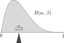
The mass of probability distribution is balanced at the expected value, here a Beta(α,β) distribution with expected value α/(α+β).
In classical mechanics, the center of mass is an analogous concept to expectation. For example, suppose X is a discrete random variable with values xi and corresponding probabilities pi. Now consider a weightless rod on which are placed weights, at locations xi along the rod and having masses pi (whose sum is one). The point at which the rod balances is E[X].
Expected values can also be used to compute the variance, by means of the computational formula for the variance
![operatorname {Var} (X)=operatorname {E} [X^{2}]-(operatorname {E} [X])^{2}.](https://wikimedia.org/api/rest_v1/media/math/render/svg/3704ee667091917e2e34f5b6e28e8d49df4b9650)
A very important application of the expectation value is in the field of quantum mechanics. The expectation value of a quantum mechanical operator  operating on a quantum state vector
  is written as
  . The uncertainty in can be calculated by the formula
  .
.
See also[edit]
- Center of mass
- Central tendency
- Chebyshev’s inequality (an inequality on location and scale parameters)
- Conditional expectation
- Expectation (the general term)
- Expectation value (quantum mechanics)
- Law of total expectation—the expected value of the conditional expected value of X given Y is the same as the expected value of X.
- Moment (mathematics)
- Nonlinear expectation (a generalization of the expected value)
- Sample mean
- Population mean
- Predicted value
- Wald’s equation—an equation for calculating the expected value of a random number of random variables
References[edit]
- ^ «Expectation | Mean | Average». www.probabilitycourse.com. Retrieved 2020-09-11.
- ^ Hansen, Bruce. «PROBABILITY AND STATISTICS FOR ECONOMISTS» (PDF). Retrieved 2021-07-20.
{{cite web}}: CS1 maint: url-status (link) - ^ Wasserman, Larry (December 2010). All of Statistics: a concise course in statistical inference. Springer texts in statistics. p. 47. ISBN 9781441923226.
- ^ History of Probability and Statistics and Their Applications before 1750. Wiley Series in Probability and Statistics. 1990. doi:10.1002/0471725161. ISBN 9780471725169.
- ^ Ore, Oystein (1960). «Ore, Pascal and the Invention of Probability Theory». The American Mathematical Monthly. 67 (5): 409–419. doi:10.2307/2309286. JSTOR 2309286.
- ^ Mckay, Cain (2019). Probability and Statistics. p. 257. ISBN 9781839473302.
- ^ George Mackey (July 1980). «HARMONIC ANALYSIS AS THE EXPLOITATION OF SYMMETRY — A HISTORICAL SURVEY». Bulletin of the American Mathematical Society. New Series. 3 (1): 549.
- ^ Huygens, Christian. «The Value of Chances in Games of Fortune. English Translation» (PDF).
- ^ Laplace, Pierre Simon, marquis de, 1749-1827. (1952) [1951]. A philosophical essay on probabilities. Dover Publications. OCLC 475539.
{{cite book}}: CS1 maint: multiple names: authors list (link) - ^ Whitworth, W.A. (1901) Choice and Chance with One Thousand Exercises. Fifth edition. Deighton Bell, Cambridge. [Reprinted by Hafner Publishing Co., New York, 1959.]
- ^ «Earliest uses of symbols in probability and statistics».
- ^ Feller 1968, p. 221.
- ^ Billingsley 1995, p. 76.
- ^ Ross 2019, Section 2.4.1.
- ^ a b Feller 1968, Section IX.2.
- ^ Papoulis & Pillai 2002, Section 5-3; Ross 2019, Section 2.4.2.
- ^ Feller 1971, Section I.2.
- ^ Feller 1971, p. 5.
- ^ Billingsley 1995, p. 273.
- ^ a b Billingsley 1995, Section 15.
- ^ Billingsley 1995, Theorems 31.7 and 31.8 and p. 422.
- ^ Billingsley 1995, Theorem 16.13.
- ^ Billingsley 1995, Theorem 16.11.
- ^ Casella & Berger 2001, p. 89; Ross 2019, Example 2.16.
- ^ Casella & Berger 2001, Example 2.2.3; Ross 2019, Example 2.17.
- ^ Billingsley 1995, Example 21.4; Casella & Berger 2001, p. 92; Ross 2019, Example 2.19.
- ^ Casella & Berger 2001, p. 97; Ross 2019, Example 2.18.
- ^ Casella & Berger 2001, p. 99; Ross 2019, Example 2.20.
- ^ Billingsley 1995, Example 21.3; Casella & Berger 2001, Example 2.2.2; Ross 2019, Example 2.21.
- ^ Casella & Berger 2001, p. 103; Ross 2019, Example 2.22.
- ^ Billingsley 1995, Example 21.1; Casella & Berger 2001, p. 103.
- ^ Johnson, Kotz & Balakrishnan 1994, Chapter 20.
- ^ Feller 1971, Section II.4.
- ^ a b c Weisstein, Eric W. «Expectation Value». mathworld.wolfram.com. Retrieved 2020-09-11.
- ^ Feller 1971, Section V.6.
- ^ Papoulis & Pillai 2002, Section 6-4.
- ^ a b Feller 1968, Section IX.6; Feller 1971, Section V.7; Papoulis & Pillai 2002, Section 5-4; Ross 2019, Section 2.8.
- ^ Feller 1968, Section IX.6.
- ^ Feller 1968, Section IX.7.
- ^ a b c d Feller 1971, Section V.8.
- ^ Billingsley 1995, pp. 81, 277.
- ^ Billingsley 1995, Section 19.
Literature[edit]
- Edwards, A.W.F (2002). Pascal’s arithmetical triangle: the story of a mathematical idea (2nd ed.). JHU Press. ISBN 0-8018-6946-3.
- Huygens, Christiaan (1657). De ratiociniis in ludo aleæ (English translation, published in 1714).
- Billingsley, Patrick (1995). Probability and measure. Wiley Series in Probability and Mathematical Statistics (Third edition of 1979 original ed.). New York: John Wiley & Sons, Inc. ISBN 0-471-00710-2. MR 1324786.
- Casella, George; Berger, Roger L. (2001). Statistical inference. Duxbury Advanced Series (Second edition of 1990 original ed.). Pacific Grove, CA: Duxbury. ISBN 0-534-11958-1.
- Feller, William (1968). An introduction to probability theory and its applications. Volume I (Third edition of 1950 original ed.). New York–London–Sydney: John Wiley & Sons, Inc. MR 0228020.
- Feller, William (1971). An introduction to probability theory and its applications. Volume II (Second edition of 1966 original ed.). New York–London–Sydney: John Wiley & Sons, Inc. MR 0270403.
- Johnson, Norman L.; Kotz, Samuel; Balakrishnan, N. (1994). Continuous univariate distributions. Volume 1. Wiley Series in Probability and Mathematical Statistics (Second edition of 1970 original ed.). New York: John Wiley & Sons, Inc. ISBN 0-471-58495-9. MR 1299979.
- Papoulis, Athanasios; Pillai, S. Unnikrishna (2002). Probability, random variables, and stochastic processes (Fourth edition of 1965 original ed.). New York: McGraw-Hill. ISBN 0-07-366011-6. (Erratum: [1])
- Ross, Sheldon M. (2019). Introduction to probability models (Twelfth edition of 1972 original ed.). London: Academic Press. doi:10.1016/C2017-0-01324-1. ISBN 978-0-12-814346-9. MR 3931305.
External links[edit]
«Expected Value | Brilliant Math & Science Wiki». brilliant.org. Retrieved 2020-08-21.
![]()
Загрузить PDF
![]()
Загрузить PDF
Ожидаемое значение — это понятие, используемое в статистике. При этом находится среднее взвешенное значение путем суммирования произведений каждого возможного результата на его вероятность. Ожидаемое значение — некая средняя величина, конкретное значение которой может не соответствовать ни одному из возможных событий: например, при бросании 6-гранной игральной кости ожидаемое значение равно 3,5. Для вычисления этого значения необходимо знать все возможные результаты и вероятность каждого из них.
Шаги
-
1
Внимательно ознакомьтесь с ситуацией. Прежде чем пронумеровать возможные события и присвоить им соответствующие вероятности, убедитесь, что учли все возможные результаты. Рассмотрим, например, игру в кости со ставкой $10. Подбрасывается 6-гранный кубик, и ваш выигрыш зависит от того, какая цифра выпала: 6 приносит выигрыш $20 (или $30 с учетом вашей ставки), 5 дает вам $10 ($20 с учетом вашей ставки), при выпадении же любой другой цифры вы ничего не выигрываете, то есть теряете свою ставку в $10.
-
2
Пронумеруйте все возможные исходы. В данном случае полезно выписать их в таблицу. В нашем примере всего 6 возможных событий: (1) выпадает 1, вы теряете $10, (2) 2 — потеря $10, (3) 3 — потеря $10, (4) 4 — потеря $10, (5) выпадает 5, и вы выигрываете $10, (6) выпадает 6, принося вам $20. Обратите внимание, что величина ставки $10 вычтена из каждого результата, то есть приведен чистый выигрыш.
-
3
Определите вероятность каждого события. В нашем примере все 6 исходов равновероятны. При бросании игрового кубика вероятность выпадения определенного номера равна 1 поделенному на 6, или 16,7 процентов. Вероятности событий также полезно внести в таблицу, особенно в случае, если они не настолько просто определяются, как в нашем примере.
-
4
Вычислите ожидаемое значение. При этом используйте выписанные вами возможные исходы и их вероятности. Воспользуйтесь следующей формулой: O1*P1 + O2*P2 + O3*P3 и так далее. Множитель «O» обозначает отдельное событие, а «P» — вероятность соответствующего события.
- В нашем примере ожидаемое значение игры в кости равно (-10 * 0,167) + (-10 * 0,167) + (-10 * 0,167) + (-10 * 0,167) + (10 * 0,167) + (20 * 0,167), или — $1,67. Таким образом, садясь играть в кости, приготовьтесь терять $1,67 в каждом раунде.
- В нашем примере ожидаемое значение игры в кости равно (-10 * 0,167) + (-10 * 0,167) + (-10 * 0,167) + (-10 * 0,167) + (10 * 0,167) + (20 * 0,167), или — $1,67. Таким образом, садясь играть в кости, приготовьтесь терять $1,67 в каждом раунде.
-
5
Подумайте о смысле ожидаемого значения. В нашем примере вероятность выигрыша была определена как — $1,67 за раунд. Такое событие, естественно, не возможно при однократном броске кости: в одном раунде вы можете потерять $10, либо выиграть $10 или $20. Тем не менее, ожидаемое значение полезно при оценке долгосрочных результатов. Если вы играете вновь и вновь, вы будете терять в среднем $1,67 за один бросок кубика. Значит, такая игра не выгодна для вас.
- Чем больше испытаний проводится, тем ближе их результат к ожидаемому значению. Например, вы сыграли 5 раз подряд и проиграли $10. Однако, если бы вы сыграли 100 раз подряд или больше, сумма вашего выигрыша или проигрыша вплотную приблизилась бы к ожидаемому значению. Это так называемый «закон больших чисел».
- Выше приведенный простой пример служит иллюстрацией того, как устроены азартные игры. Ваш усредненный выигрыш отрицателен, что означает выгоду для игрового дома. Тем не менее, азарт и надежда на крупный выигрыш привлекают все новых игроков.
Реклама


Советы
- При наличии большого количества возможных событий вы можете создать электронную таблицу, занося в нее события и их вероятности.
- В приведенном выше примере можно использовать и другие денежные единицы, цифры от этого не изменятся.
Реклама
Что вам понадобится
- Карандаш
- Лист бумаги
- Калькулятор
Об этой статье
Эту страницу просматривали 10 691 раз.
Была ли эта статья полезной?
17 авг. 2022 г.
читать 2 мин
Распределение вероятностей говорит нам о вероятности того, что случайная величина примет определенные значения.
Например, следующее распределение вероятностей говорит нам о вероятности того, что определенная футбольная команда забьет определенное количество голов в данной игре:
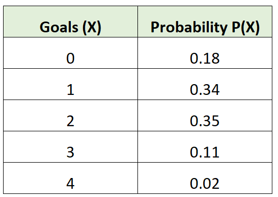
Чтобы найти ожидаемое значение распределения вероятностей, мы можем использовать следующую формулу:
μ = Σx * P (x)
куда:
- х: значение данных
- P(x): вероятность ценности
Например, ожидаемое количество голов для футбольной команды будет рассчитано как:
μ = 0*0,18 + 1*0,34 + 2*0,35 + 3*0,11 + 4*0,02 = 1,45 гола.
В следующем примере представлен пошаговый пример расчета ожидаемого значения распределения вероятностей в Excel.
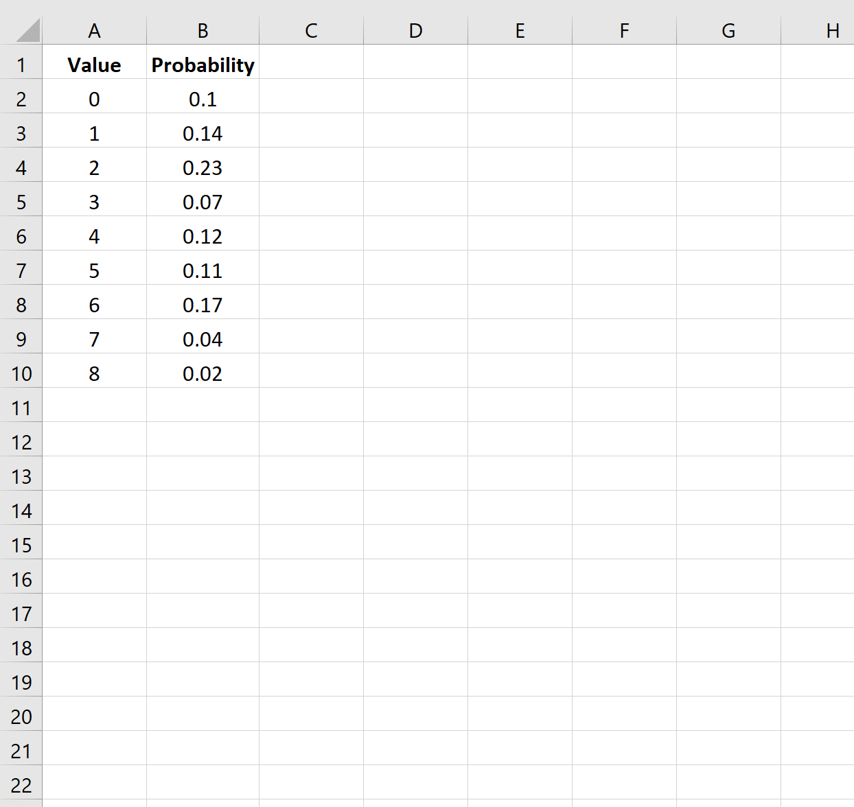
Шаг 1: введите данные
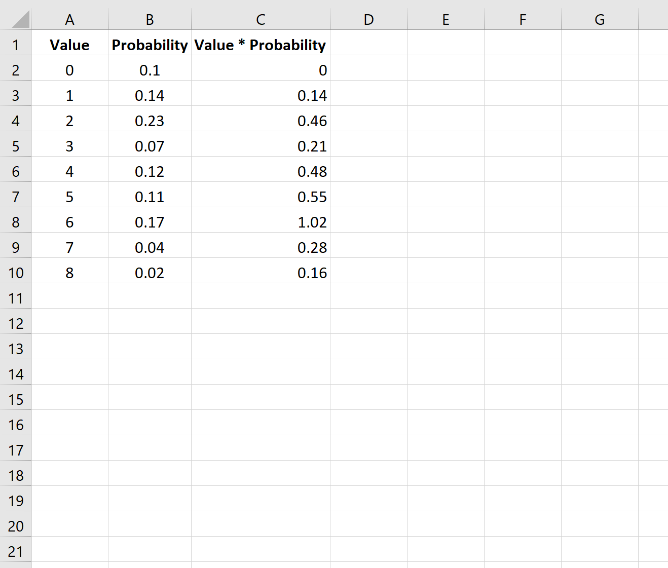
Во-первых, давайте введем значения данных и соответствующие вероятности для данного распределения вероятностей:
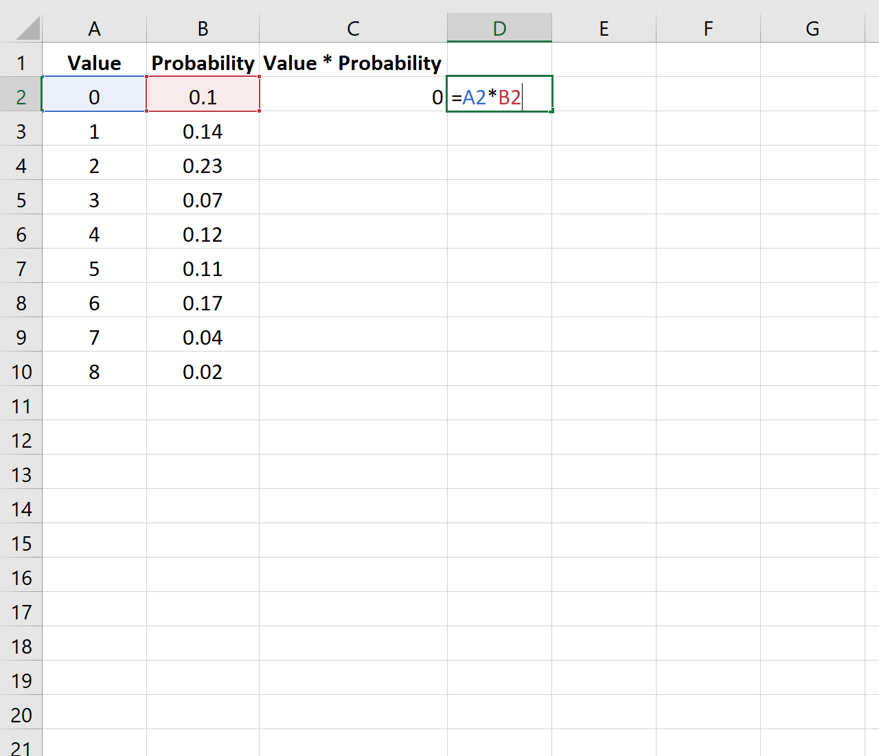
Шаг 2: Умножьте значения и вероятности
Затем мы умножим первое число в столбце «Значения» на первое число в столбце «Вероятность»:
Затем мы скопируем и вставим эту формулу в каждую ячейку столбца C:
Шаг 3: Рассчитайте ожидаемое значение
Наконец, мы можем рассчитать ожидаемое значение распределения вероятностей, используя SUM(C2:C10) для суммирования всех значений в столбце C:
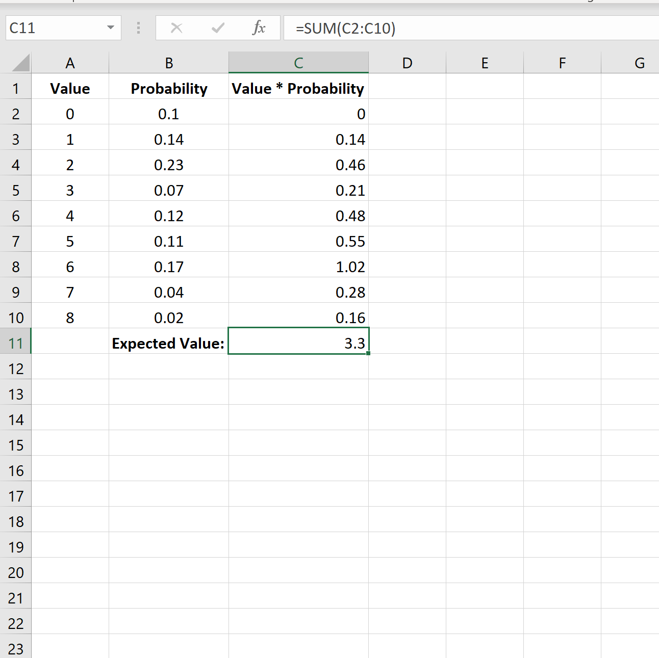
Ожидаемое значение для этого распределения вероятностей равно 3,3 .
Дополнительные ресурсы
В следующих руководствах объясняется, как рассчитать другую описательную статистику в Excel:
Как найти среднее значение, медиану и моду в Excel
Как рассчитать межквартильный диапазон в Excel
Как рассчитать коэффициент вариации в Excel
Написано
![]()
Замечательно! Вы успешно подписались.
Добро пожаловать обратно! Вы успешно вошли
Вы успешно подписались на кодкамп.
Срок действия вашей ссылки истек.
Ура! Проверьте свою электронную почту на наличие волшебной ссылки для входа.
Успех! Ваша платежная информация обновлена.
Ваша платежная информация не была обновлена.
Как найти математическое ожидание?
Математическое ожидание случайной величины $X$ (обозначается $M(X)$ или реже $E(X)$) характеризует среднее значение случайной величины (дискретной или непрерывной). Мат. ожидание — это первый начальный момент заданной СВ.
Математическое ожидание относят к так называемым характеристикам положения распределения (к которым также принадлежат мода и медиана). Эта характеристика описывает некое усредненное положение случайной величины на числовой оси. Скажем, если матожидание случайной величины — срока службы лампы, равно 100 часов, то считается, что значения срока службы сосредоточены (с обеих сторон) от этого значения (с тем или иным разбросом, о котором уже говорит дисперсия).
Нужна помощь? Решаем теорию вероятностей на отлично
Лучшее спасибо — порекомендовать эту страницу
Формула среднего случайной величины
Математическое ожидание дискретной случайной величины Х вычисляется как сумма произведений значений $x_i$ , которые принимает СВ Х, на соответствующие вероятности $p_i$:
$$
M(X)=sum_{i=1}^{n}{x_i cdot p_i}.
$$
Для непрерывной случайной величины (заданной плотностью вероятностей $f(x)$), формула вычисления математического ожидания Х выглядит следующим образом:
$$
M(X)=int_{-infty}^{+infty} f(x) cdot x dx.
$$
Пример нахождения математического ожидания
Рассмотрим простые примеры, показывающие как найти M(X) по формулам, введеным выше.
Пример 1. Вычислить математическое ожидание дискретной случайной величины Х, заданной рядом:
$$
x_i quad -1 quad 2 quad 5 quad 10 quad 20 \
p_i quad 0.1 quad 0.2 quad 0.3 quad 0.3 quad 0.1
$$
Используем формулу для м.о. дискретной случайной величины:
$$
M(X)=sum_{i=1}^{n}{x_i cdot p_i}.
$$
Получаем:
$$
M(X)=sum_{i=1}^{n}{x_i cdot p_i} =-1cdot 0.1 + 2 cdot 0.2 +5cdot 0.3 +10cdot 0.3+20cdot 0.1=6.8.
$$
Вот в этом примере 2 описано также нахождение дисперсии Х.
Пример 2. Найти математическое ожидание для величины Х, распределенной непрерывно с плотностью $f(x)=12(x^2-x^3)$ при $x in(0,1)$ и $f(x)=0$ в остальных точках.
Используем для нахождения мат. ожидания формулу:
$$
M(X)=int_{-infty}^{+infty} f(x) cdot x dx.
$$
Подставляем из условия плотность вероятности и вычисляем значение интеграла:
$$
M(X)=int_{-infty}^{+infty} f(x) cdot x dx = int_{0}^{1} 12(x^2-x^3) cdot x dx = int_{0}^{1} 12(x^3-x^4) dx = \
=left.(3x^4-frac{12}{5}x^5) right|_0^1=3-frac{12}{5} = frac{3}{5}=0.6.
$$
Другие задачи с решениями по ТВ
Подробно решим ваши задачи по теории вероятностей
Вычисление математического ожидания онлайн
Как найти математическое ожидание онлайн для произвольной дискретной случайной величины? Используйте калькулятор ниже.
- Введите число значений случайной величины К.
- Появится форма ввода для значений $x_i$ и соответствующих вероятностей $p_i$ (десятичные дроби вводятся с разделителем точкой, например: -10.3 или 0.5). Введите нужные значения (проверьте, что сумма вероятностей равна 1, то есть закон распределения корректный).
- Нажмите на кнопку «Вычислить».
- Калькулятор покажет вычисленное математическое ожидание $M(X)$.
Видео. Полезные ссылки
Видеоролики: что такое среднее (математическое ожидание)
Если вам нужно более подробное объяснение того, что такое мат.ожидание, как она вычисляется и какими свойствами обладает, рекомендую два видео (для дискретной и непрерывной случайной величины соответственно).
Лучшее спасибо — порекомендовать эту страницу
Полезные ссылки
А теперь узнайте о том, как находить дисперсию или проверьте онлайн-калькулятор для вычисления математического ожидания, дисперсии и среднего квадратического отклонения дискретной случайной величины.
Что еще может пригодиться? Например, для изучения основ теории вероятностей — онлайн учебник по терверу. Для закрепления материала — еще примеры решений по теории вероятностей.
А если у вас есть задачи, которые надо срочно сделать, а времени нет? Можете поискать готовые решения в решебнике или заказать в МатБюро:
Ожидаемое значение случайной величины является важным количественным понятием в инвестициях. Инвесторы постоянно используют ожидаемые значения — при оценке выгод от альтернативных инвестиций, при прогнозировании прибыли на акцию и других корпоративных финансовых величин и коэффициентов, а также при оценке любых других факторов, которые могут повлиять на их финансовое положение.
Ожидаемое значение случайной величины определяется следующим образом:
Определение ожидаемого значения.
Ожидаемое значение случайной величины (или математическое ожидание, от англ. ‘expected value’) является средневзвешенной вероятностью возможных результатов случайной величины.
Для случайной величины (X) математическое ожидание (X) обозначается как (E(X)).
Ожидаемое значение (например, ожидаемая доходность акций) представляет собой либо будущее значение, например прогноз, либо «истинное» значение среднего (например, среднее значение для генеральной совокупности, которое обсуждается в чтении о статистических концепциях и доходности рынка). Следует различать ожидаемое значение и понятия исторического или выборочного среднего.
Выборочное среднее также суммирует в единственном числе центральное значение выборки. Тем не менее, выборочное среднее представляет собой центральное значение для определенного набора наблюдений в виде равно взвешенного среднего значения этих наблюдений.
Пример (8) анализа прибыли на акцию BankCorp.
Вы продолжаете свой анализ прибыли на акцию (EPS) BankCorp. В Таблице (3) вы представили распределение вероятностей для EPS BankCorp за текущий финансовый год.
|
Вероятность |
EPS ($) |
|---|---|
|
0.15 |
2.60 |
|
0.45 |
2.45 |
|
0.24 |
2.20 |
|
0.16 |
2.00 |
|
1.00 |
Каково ожидаемое значение EPS BankCorp на текущий финансовый год?
Следуя определению математического ожидания, перечислите каждый результат, взвесьте его по вероятности и суммируйте взвешенные результаты.
( begin{aligned}
E(EPS) &= 0.15($2.60) + 0.45($2.45) + 0.24($2.20) + 0.16($2.00) \
&= $2.3405
end{aligned} )
Ожидаемое значение EPS составляет $2.34.
Формула, которое суммирует ваши вычисления в Примере (8):
( dst large begin{aligned}
E(X) &= P(X_l)X_l + P(X_2)X_2 + cdots + P (X_n)X_n \
&= dsum_{i=1}^{n}P(X_i)X_i
end{aligned} ) (Формула 7)
где
(X_i) — один из (n) возможных результатов случайной величины (X).
Для простоты мы моделируем все случайные величины в этом чтении как дискретные случайные величины, которые имеют исчисляемый набор результатов. Для непрерывных случайных величин, которые обсуждаются вместе с дискретными случайными величинами в чтении об общих распределениях вероятностей, операция, соответствующая суммированию, является интегрированием.
Ожидаемое значение — это наш прогноз. Поскольку мы обсуждаем случайные величины, мы не можем рассчитывать на реализацию отдельного прогноза (хотя мы надеемся, что в среднем прогнозы будут точными).
В результате важно измерить риск, с которым мы сталкиваемся. Дисперсия и стандартное отклонение случайной величины измеряют разброс результатов вокруг ожидаемого значения или прогноза.
Определение дисперсии случайной величины.
Дисперсия случайной величины (англ. ‘variance of random variable’) — это ожидаемое значение (средневзвешенное по вероятности) квадратов отклонений от ожидаемого значения случайной величины:
( large dst
sigma^2(X) = E Big { big [ X — E(X) big ]^2 Big } ) (Формула 
Для дисперсии случайной величины используются два обозначения:
( sigma^2(X) ) и ( mathrm{Var}(X) )
- Дисперсия — это число, которое больше или равно 0, потому что это сумма квадратов.
- Если дисперсия равна 0, дисперсия или риск отсутствуют.
- Результат определенный, а величина (X) вовсе не случайна.
- Дисперсия случайной величины больше 0 указывает на дисперсию (т.е. разброс) результатов.
- Увеличение дисперсии случайной величины указывает на увеличение разброса результатов.
Дисперсия (X) — это величина, выраженная в квадратах единиц (X). Например, если случайная величина является процентной доходностью, дисперсия доходности выражается в процентах, возведенных в квадрат.
Стандартное отклонение случайной величины легче интерпретировать, чем дисперсию, поскольку оно выражено в тех же единицах, что и случайная величина. Если случайная величина выражена в процентах, то стандартное отклонение также будет выражено в процентах.
Обратите внимание, что в следующем примере там, где дисперсия доходности указывается в виде десятичной дроби, усложнения работы с «процентами в квадрате» не возникает.
Определение стандартного отклонения случайной величины.
Стандартное отклонение случайной величины (англ. ‘standard deviation of random variable’) — это положительный квадратный корень дисперсии случайной величины.
Лучший способ познакомиться с этими понятиями — это поработать с ними на примерах.
Пример (9) расчета дисперсии и стандартного отклонения для EPS BankCorp.
В Примере (8) вы рассчитали ожидаемое значение прибыли на акцию (EPS) BankCorp как $2.34, что является вашим прогнозом.
Теперь вы хотите измерить разброс вокруг вашего прогноза. В Таблице 4 показано ваше представление о вероятности распределения прибыли на акцию за текущий финансовый год.
|
Вероятность |
EPS ($) |
|---|---|
|
0.15 |
2.60 |
|
0.45 |
2.45 |
|
0.24 |
2.20 |
|
0.16 |
2.00 |
|
1.00 |
Каковы дисперсия и стандартное отклонение EPS BankCorp для текущего финансового года?
Порядок расчета всегда предполагает сначала расчет ожидаемого значения, затем дисперсии, затем стандартное отклонение. Ожидаемое значение уже рассчитано.
Следуя приведенному выше определению дисперсии, рассчитайте отклонение каждого результата от среднего или ожидаемого значения, возведите в квадрат каждое отклонение, вычислите вес (умножьте) каждое квадратичное отклонение на вероятность его возникновения, а затем сложите эти результаты.
( small begin{aligned}
sigma^2(EPS) &= P($2.60)[$2.60 — E(EPS)]^2 + P($2.45)[$2.45 — E(EPS)]^2 \
&+ P($2.20)[$2.20 — E(EPS)]^2 + P($2.00)[$2.00 — E(EPS)]^2 \
&= 0.15(2.60 — 2.34)^2 + 0.45(2.45 — 2.34)^2 \
&+ 0.24(2.20 — 2.34)^2 + 0.16(2.00 — 2.34)^2 \
&= 0.01014 + 0.005445 + 0.004704 + 0.018496 = 0.038785
end{aligned} )
Стандартное отклонение — это положительный квадратный корень из 0.038785:
( sigma(EPS) = 0.038785^{1/2} = 0.196939 )
или приблизительно 0.20.
Формулой, с помощью которой выполняется ваш расчет дисперсии в Примере 9 будет:
(Формула 9)
(
begin{aligned}
sigma^2(X) &= P(X_l)big[ X_l — E(X) big]^2 + P(X_2)big[ X_2 — E(X) big]^2 \
&+ cdots + P(X_n)big[ X_n — E(X) big]^2 = \
&sum_{i=1}^{n}P(X_i) big[ X_i — E(X) big]^2
end{aligned} )
где
(X_i) — один из (n) возможных результатов случайной величины (X).
В инвестициях мы используем любую соответствующую информацию, доступную для составления наших прогнозов. Когда мы уточняем наши ожидания или прогнозы, мы обычно вносим корректировки на основе новой информации или событий; в этих случаях мы используем условные ожидаемые значения (англ. ‘conditional expected values’).
Ожидаемое значение случайной величины (X) для данного события или сценария ( S ) обозначается как ( E(X|S) ).
Предположим, что случайная величина (X) может принимать любое из (n) различных результатов ( X_1, X_2, …, X_n ) (эти результаты образуют набор взаимоисключающих и исчерпывающих событий).
Ожидаемое значение (X) при условии (S) — это первый результат, (X_i), умноженный на вероятность первого результата, заданного(S), ( P(X_1|S) ), плюс второй результат, (X_2), умноженный на вероятность второго результата, заданного (S), ( P(X_2|S) ) и так далее.
(Формула 10)
( large begin{aligned}
E(X|S) &= P(X_1|S)X_1 + P(X_2|S)X_2 \
&+ ldots + P(X_n|S)X_n
end{aligned} )
Мы проиллюстрируем эту формулу далее.
Параллельно с правилом полной вероятности для определения безусловных вероятностей существует принцип для определения (безусловных) ожидаемых значений.
Этот принцип является правилом полной вероятности для ожидаемого значения (англ. ‘total probability rule for expected value’).
Правило общей вероятности для ожидаемого значения.
( large E(X) = E(X|S)P(S) + E(X|S^C)P(S^C) ) (Формула 11)
(Формула 12)
( large begin{aligned}
E(X) &= E(X|S_1)P(S_1) + E(X|S_2)P(S_2) \
&+ ldots + E(X|S_n)P(S_n)
end{aligned} )
где
- ( S_1, S_2, ldots, S_n ) — взаимоисключающие и исчерпывающие сценарии или события.
Формула 12, гласит, что ожидаемое значение (X) равно ожидаемому значению (X) для данного сценария 1, ( E(X|S_1) ), умноженному на вероятность сценария 1, ( P(S_1) ) плюс ожидаемое значение (X) для данного сценария 2, ( E(X|S_2) ), умноженное на вероятность сценария 2, ( P(S_2) ) и т.д.
Чтобы использовать этот принцип, мы формулируем взаимоисключающие и исчерпывающие сценарии, которые полезны для понимания результатов случайной величины. Этот подход был использован при разработке распределения вероятностей EPS в BankCorp в Примерах 8 и 9, которое мы сейчас обсудим.
Доходы BankCorp чувствительны к процентным ставкам, и корпорация получает выгоду в условиях снижения процентных ставок.
Предположим, есть вероятность 0.60, что BankCorp будет работать в условиях снижения процентных ставок в текущем финансовом году, и вероятность 0.40, что она будет работать в условиях стабильных процентных ставок (вероятность повышения процентных ставок оценивается как незначительная).
Если происходит снижение процентных ставок, вероятность того, что EPS составит $2.60, оценивается в 0.25, а вероятность того, что EPS составит $2.45, оценивается в 0.75.
Обратите внимание, что 0.60, вероятность снижения процентных ставок, умноженная на 0.25, вероятность EPS в $2.60 при условии снижения процентной ставки равна 0.15, (безусловная) вероятность $2.60 приведена в таблице в Примерах 8 и 9. Вероятности последовательны.
Кроме того, 0.60(0.75) = 0.45, вероятность прибыли на акцию в размере $2.45 приведена в Таблицах 3 и 4.
Древовидная диаграмма на Рисунке 2 показывает остальную часть анализа.
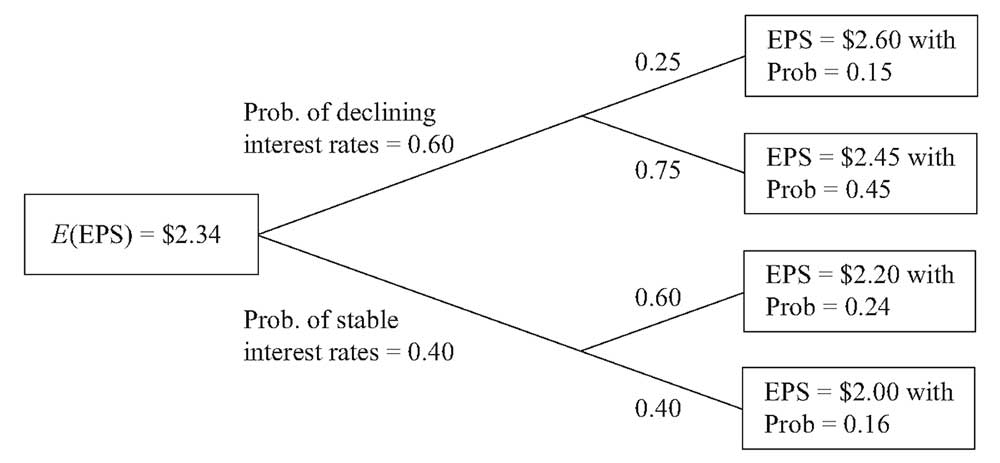 Рисунок 2. Анализ прогнозируемой прибыли на акцию (EPS) BankCorp.
Сценарий снижения процентных ставок указывает нам на узел дерева, который разветвляется до результатов в $2.60 и $2.45. Мы можем найти ожидаемую прибыль на акцию при условии снижения процентной ставки, используя Формулу 10, следующим образом:
E (EPS | Снижение процентных ставок) =
= 0.25($2.60) + 0.75($2.45) = $2.4875
Если процентные ставки стабильны,
E(EPS | Стабильные процентные ставки) =
= 0.60($2.20) + 0.40($2.00) = $2.12
Например, как только мы получаем новую информацию о том, что процентные ставки стабильны, мы пересматриваем наши первоначальные ожидания EPS с $2.34 вниз до $2.12.
Теперь, используя правило общей вероятности для ожидаемого значения, находим:
E(EPS) = E(EPS | Снижение процентных ставок) P(Снижение процентных ставок) + E(EPS | Стабильные процентные ставки) P(Стабильные процентные ставки)
Таким образом,
( E(EPS) = $2.4875(0.60) + $2.12(0.40) = $2.3405 )
или около $2.34.
Эта сумма идентична оценке ожидаемого значения EPS, рассчитанной непосредственно из распределения вероятностей в Примере 8. Так же, как и наши вероятности, ожидаемые значения должны быть согласующимися; в противном случае наши инвестиционные действия могут создать возможности получения прибыли для других инвесторов за наш счет.
Для анализа мы сначала разрабатываем факторы или сценарии, которые влияют на результат интересующего события. После присвоения вероятностей этим сценариям мы формируем ожидания, обусловленные различными сценариями.
Затем мы действуем в обратном направлении, чтобы получить ожидаемую стоимость на текущий момент. В рассмотренном выше примере EPS был интересующим нас событием, а изменение процентных ставок было фактором, влияющим на EPS.
Мы также можем рассчитать дисперсию EPS для каждого сценария:
(sigma^2)(EPS | Снижение процентных ставок)
= P(
$2.60 | Снижение процентных ставок)
(times)[$2.60 — E(EPS | Снижение процентных ставок)]2
+ P($2.45 | Снижение процентных ставок)
(times)[$2.45 — E(EPS | Снижение процентных ставок)]2
= 0.25(2.60 — $2.4875)2 + 0.75(2.45 — $2.4875)2 = 0.004219
(sigma^2)(EPS | Стабильные процентные ставки)
= P(
$2.20 | Стабильные процентные ставки)
(times) [$2.20 — E(EPS | Стабильные процентные ставки)]2
+ P($2.00 | Стабильные процентные ставки)
(times) [$2.00 — E(EPS | Стабильные процентные ставки)]2
= 0.60(2.20 — $2.12)2 + 0.40(2.00 — $2.12)2 = 0.0096
Это условные стандартные отклонения, т.е. дисперсия EPS при условии снижения процентных ставок и дисперсия EPS при условии стабильных процентных ставок. Связь между безусловной дисперсией и условной дисперсией является относительно сложной темой.
Безусловная дисперсия EPS представляет собой сумму двух слагаемых:
- ожидаемого значения (средневзвешенного по вероятности) условных дисперсий и
- дисперсии условных ожидаемых значений EPS.
Второе слагаемое возникает потому, что изменчивость условного ожидаемого значения является источником риска.
Первое слагаемое равно:
(sigma^2)(EPS) = P(Снижение процентных ставок) (sigma^2)(EPS | Снижение процентных ставок) + P(Стабильные процентные ставки) (sigma^2)(EPS | Стабильные процентные ставки)
= 0.60(0.004219) + 0.40(0.0096) = 0.006371
Второе слагаемое равно:
(sigma^2)[E(EPS | Среда процентных ставок)] =
0.60($2.4875 — $2.34)2 + 0.40($2.12 — $2.34)2 = 0.032414
Суммируя два слагаемых, находим безусловную дисперсию, которая равна:
0.006371 + 0.032414 = 0.038785
Основными моментами здесь является:
- то, что дисперсия, как и ожидаемое значение, имеет условный аналог безусловной концепции и
- то, что мы можем использовать условную дисперсию для оценки риска по конкретному сценарию.
Пример (10) анализа прибыли на акцию BankCorp.
Продолжая анализ показателей BankCorp, вы сосредоточитесь сейчас на структуре затрат BankCorp. Модель операционных расходов BankCorp, которую вы исследуете, это:
( hat{Y} = a + bX )
где
- ( hat{Y} ) — прогноз операционных расходов в млн. долларов, а
- X — количество филиалов корпорации
( hat{Y} ) представляет собой ожидаемое значение (Y) при условии (X) или (E (Y|X)).
(( hat{Y} ) — это обозначение, используемое в регрессионном анализе, который мы обсудим в следующих чтениях.)
Вы интерпретируете значение (a) как постоянные затраты, а (b) — как переменные затраты. Уравнение будет выглядеть следующим образом:
( hat{Y} = 12.5 + 0.65X )
BankCorp в настоящее время имеет 66 филиалов, и, согласно уравнению:
12.5 + 0.65(66) = $55.4 млн.
У вас есть два сценария роста, изображенные на древовидной диаграмме на Рисунке 3.
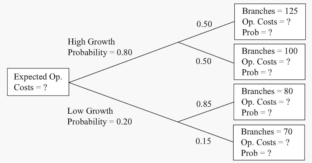 Рисунок 3. Прогнозируемые операционные расходы BankCorp.
- Рассчитайте прогнозируемые операционные расходы с учетом различных уровней операционных расходов, используя уравнение ( hat{Y} = 12.5 + 0.65X ). Укажите вероятность каждого уровня из числа филиалов (см. вопросительные знак в крайних правых полях древовидной диаграммы).
- Рассчитайте ожидаемую стоимость операционных расходов в сценарии с высокими темпами роста. Также рассчитайте ожидаемую стоимость операционных расходов по сценарию низкого роста.
- Ответьте на вопрос в начальном поле дерева: каковы ожидаемые операционные расходы BankCorp?
Решение для части 1:
Используя уравнение ( hat{Y} = 12.5 + 0.65X ) для ветвей дерева сверху вниз, находим:
|
Операционные расходы |
Вероятность |
|---|---|
|
( hat{Y}) = 12.5 + 0.65(125) = $93.75 млн. |
0.80(0.50) = 0.40 |
|
( hat{Y}) = 12.5 + 0.65(100) = $77.50 млн. |
0.80(0.50) = 0.40 |
|
( hat{Y}) = 12.5 + 0.65(80) = $64.50 млн. |
0.20(0.85) = 0.17 |
|
( hat{Y}) = 12.5 + 0.65(70) = $58.00 млн. |
0.20(0.15) = 0.03 |
|
Сумма = 1.00 |
Решение для части 2:
Суммы представлены в млн. долл.
E(операционные расходы | высокий рост) =
= 0.50(93.75) + 0.50(77.50) = $85.625
E(операционные расходы | низкий рост) =
= 0.85(64.50) + 0.15(58.00) = $63.525
Решение для части 3:
Суммы представлены в млн. долл.
E(операционные расходы) = E(операционные расходы | высокий рост) P(высокий рост)
+ E(операционные расходы | низкий рост) P(низкий рост)
= $85.625(0.80) + $63.525(0.20) = $81.205
Ожидаемые операционные расходы BankCorp составляют $81.205.
Мы снова увидим условные вероятности, когда будем обсуждать формулу Байеса. В этом разделе представлено несколько примеров проблем, которые можно решить с помощью вероятностных концепций.
Следующая проблема опирается на эти концепции, а также на аналитические навыки.
Пример (11) расчета премии за риск дефолта для долгового инструмента за один период.
Как соуправляющий портфеля краткосрочных облигаций, вы пересматриваете цену спекулятивной (дисконтной) облигации с нулевым купоном и сроком обращения 1 год. Для этого типа облигаций доход представляет собой разницу между уплаченной суммой и номинальной стоимостью, полученной при погашении.
Ваша цель — оценить соответствующую премию за риск дефолта для этой облигации. Вы определяете премию за риск дефолта как дополнительную доходность сверх безрисковой доходности, которая будет компенсировать инвесторам риск дефолта.
Если (R) — это обещанная доходность (доходность к погашению) по долговому инструменту, а (R_F) — безрисковая ставка, то премия за риск дефолта — это (R — R_F).
Вы оцениваете вероятность того, что риск дефолта облигации, обозначаемый как P(дефолт облигации) = 0,06.
Анализируя текущую доходность денежного рынка, вы обнаруживаете, что однолетние казначейские векселя США (T-bills) обеспечивают доходность в 2%, и вы используете эту ставку как (R_F).
В качестве первого шага вы делаете упрощенное предположение, что держатели облигаций ничего не возместят в случае дефолта.
Какая минимальная премия за риск вам требуется для этого инструмента?
Основная сложность в решении этого типа проблемы состоит в том, чтобы найти отправную точку. Во многих проблемах, включая эту, эффективным первым шагом является разделение возможных результатов на взаимоисключающие и исчерпывающие события экономически логичным способом.
Здесь, с точки зрения держателя облигации, есть два события, которые влияют на доходность, это:
- дефолт облигации и
- то, что дефолт облигации не произошел.
Эти два события охватывают все результаты.
Как эти события влияют на доход владельца облигации?
Вторым шагом является вычисление стоимости облигации для двух событий. У нас нет конкретных данных по номинальной стоимости облигации, но мы можем рассчитать стоимость за $1 или на одну вложенную денежную единицу.
|
Дефолт облигации |
Дефолт облигации не произошел |
|
|---|---|---|
|
Стоимость облигации |
$0 |
$(1 + R) |
Третий шаг — найти ожидаемую стоимость облигации (на 1 вложенный $).
E(Облигация) = $0 (times) P(Дефолт облигации) + $(1 + (R)) [1 — P(Дефолт облигации не произошел)]
Таким образом,
E(Облигация) = $(1 + (R)) [1 — P(Дефолт облигации)].
Ожидаемая стоимость безрискового казначейский вексель (Т-bill) на 1 вложенный $ составляет ( (1 + R_F) ).
Следующий шаг требует экономических суждений.
Вы хотите, чтобы премия за риск была достаточно большой, поэтому вы ожидаете, по крайней мере, безубыточности по сравнению с инвестированием в T-bill. Этот результат будет достигнут, если ожидаемая стоимость облигации будет равна ожидаемой стоимости Т-bill за 1 вложенный $.
Ожидаемая стоимость облигации = Ожидаемая стоимость T-Bill
$(1 + (R))[1 — P(Дефолт облигации) = (1 + (R_F))
Рассчитывая доход к погашению по облигации, вы найдете:
(R) = {(1 + (R_F))/[1 — P(Дефолт облигации)]} — 1
Подставляя в значения формулу, вы получите:
(R) = [1.02/(1 — 0.06)] — 1 = 1.08511 — 1 = 0.08511
или около 8.51%, а премия за риск дефолта составит
(R — R_F) = 8.51% — 2% = 6.51%.
Вам необходима премия за риск дефолта не менее 651 базисных пунктов. Вы можете заявить об этом следующим образом: если цена облигации составляет 8.51%, вы получите спред в 651 базисный пункт, а также получите номинальную сумму облигации с вероятностью 94%.
Однако, если произойдет дефолт, вы потеряете все. С премией в 651 базисный пункт, вы рассчитываете точку безубыточности относительно инвестиций в казначейские векселя. Поскольку инвестиции в облигации с нулевым купоном имеют переменную стоимость, если вы не склонны к риску, вы будете требовать, чтобы премия превышала 651 базисный пункт.
Этот анализ является отправной точкой. Владельцы облигаций обычно возмещают часть своих инвестиций в случае дефолта. Следующим шагом будет включение в анализ уровня возмещения средств в случае дефолта.
В этом разделе мы рассматривали случайные финансовые величины, такие как EPS, как отдельные значения. Мы не исследовали, как такие показатели, как ожидаемое значение и дисперсия EPS, могут быть функциями других случайных величин.
Доходность портфеля — это одна случайная величина, которая, очевидно, является функцией других случайных величин — случайных ставок доходности отдельных ценных бумаг в портфеле.
Чтобы проанализировать ожидаемую доходность портфеля и дисперсию доходности, мы должны понимать, что эти величины являются функцией характеристик доходности отдельных ценных бумаг. Глядя на дисперсию доходности портфеля, мы видим, что способ, которым меняется доходность каждой отдельной ценной бумаги меняется, чрезвычайно важен.
Чтобы понять значение этих изменений отдельных ценных бумаг портфеля, нам необходимо изучить некоторые новые концепции, — ковариацию и корреляцию. В следующем разделе, который касается ожидаемой доходности портфеля и дисперсии доходности, эти концепции будут рассмотрены.