Как найти передаточную функцию в матлабе - Исправление недочетов и поиск решений вместе с Examum.ru

tf

Description

Use tf to create real-valued or complex-valued transfer
function models, or to convert dynamic system
models to transfer function form.

Transfer functions are a frequency-domain representation of linear time-invariant
systems. For instance, consider a continuous-time SISO dynamic system represented by the
transfer function sys(s) = N(s)/D(s), where s = jw
and N(s) and D(s) are called the numerator and
denominator polynomials, respectively. The tf model object can
represent SISO or MIMO transfer functions in continuous time or discrete time.

You can create a transfer function model object either by specifying its coefficients
directly, or by converting a model of another type (such as a state-space model
ss) to transfer-function form. For more information, see Transfer Functions.

You can also use tf to create generalized state-space (genss) models or uncertain state-space (uss (Robust Control Toolbox)) models.

Creation

Syntax

Description

example

sys = tf(numerator,denominator)
creates a continuous-time transfer function model, setting the
Numerator and Denominator
properties. For instance, consider a continuous-time SISO dynamic system
represented by the transfer function sys(s) = N(s)/D(s),
the input arguments numerator and
denominator are the coefficients of
N(s) and D(s),
respectively.

example

sys = tf(numerator,denominator,ts)
creates a discrete-time transfer function model, setting the
Numerator, Denominator, and
Ts properties. For instance, consider a
discrete-time SISO dynamic system represented by the transfer function
sys(z) = N(z)/D(z), the input arguments
numerator and denominator are
the coefficients of N(z) and D(z),
respectively. To leave the sample time unspecified, set
ts input argument to -1.

example

sys = tf(numerator,denominator,ltiSys)
creates a transfer function model with properties inherited from the dynamic
system model ltiSys, including the sample time.

example

sys = tf(m)
creates a transfer function model that represents the static gain,
m.

example

sys = tf(___,Name,Value)
sets properties of the transfer function model using one or more
Name,Value pair arguments for any of the previous
input-argument combinations.

example

sys = tf(ltiSys)
converts the dynamic system model ltiSys to a transfer
function model.

example

sys = tf(ltiSys,component)
converts the specified component of
ltiSys to transfer function form. Use this syntax
only when ltiSys is an identified linear time-invariant
(LTI) model.

example

s = tf('s') creates special variable
s that you can use in a rational expression to create
a continuous-time transfer function model. Using a rational expression can
sometimes be easier and more intuitive than specifying polynomial
coefficients.

example

z = tf('z',ts) creates special
variable z that you can use in a rational expression to
create a discrete-time transfer function model. To leave the sample time
unspecified, set ts input argument to
-1.

Input Arguments

expand all

`numerator` — Numerator coefficients of the transfer function
row vector | `Ny`-by-`Nu` cell array of row
vectors

Numerator coefficients of the transfer function, specified as:

A row vector of polynomial coefficients.
An Ny-by-Nu cell array
of row vectors to specify a MIMO transfer function, where
Ny is the number of outputs, and
Nu is the number of inputs.

When you create the transfer function, specify the numerator
coefficients in order of descending power. For instance, if the transfer
function numerator is 3s^2-4s+5, then specify
numerator as [3 -4 5]. For a
discrete-time transfer function with numerator 2z-1,
set numerator to [2 -1].

Also a property of the tf object. For more
information, see Numerator.

`denominator` — Denominator coefficients of the transfer function
row vector | `Ny`-by-`Nu` cell array of row
vectors

Denominator coefficients, specified as:

A row vector of polynomial coefficients.
An Ny-by-Nu cell array
of row vectors to specify a MIMO transfer function, where
Ny is the number of outputs and
Nu is the number of inputs.

When you create the transfer function, specify the denominator
coefficients in order of descending power. For instance, if the transfer
function denominator is 7s^2+8s-9, then specify
denominator as [7 8 -9]. For
a discrete-time transfer function with denominator
2z^2+1, set denominator to
[2 0 1].

Also a property of the tf object. For more
information, see Denominator.

`ts` — Sample time
scalar

Sample time, specified as a scalar. Also a property of the
tf object. For more information, see Ts.

`ltiSys` — Dynamic system
dynamic system model | model array

Dynamic system, specified as a SISO or MIMO dynamic
system model or array of dynamic system models. Dynamic
systems that you can use include:

Continuous-time or discrete-time numeric LTI models, such as
tf, zpk, ss, or
pid
models.
Generalized or uncertain LTI models such as genss or
uss (Robust Control Toolbox) models.
(Using uncertain models requires Robust Control Toolbox™ software.)

The resulting transfer function assumes
- current values of the tunable components for tunable
  control design blocks.
- nominal model values for uncertain control design
  blocks.
Identified LTI models, such as idtf (System Identification Toolbox), idss (System Identification Toolbox), idproc (System Identification Toolbox),
idpoly (System Identification Toolbox), and
idgrey (System Identification Toolbox) models.
To select the component of the identified model to convert,
specify component. If you do not specify
component, tf
converts the measured component of the identified model by
default. (Using identified models
requires System Identification Toolbox™ software.)

`m` — Static gain
scalar | matrix

Static gain, specified as a scalar or matrix. Static gain or steady
state gain of a system represents the ratio of the output to the input
under steady state condition.

`component` — Component of identified model
`'measured'` (default) | `'noise'` | `'augmented'`

Component of identified model to convert, specified as one of the
following:

'measured' — Convert the measured component
of sys.
'noise' — Convert the noise component of
sys
'augmented' — Convert both the measured and
noise components of sys.

component only applies when
sys is an identified LTI model.

For more information on identified LTI models and their measured and
noise components, see Identified LTI Models.

Output Arguments

expand all

`sys` — Output system model
`tf` model object | `genss` model object | `uss` model object

Output system model, returned as:

A transfer function (tf) model object,
when numerator and
denominator input arguments are
numeric arrays.
A generalized state-space model (genss)
object, when the numerator or
denominator input arguments
includes tunable parameters, such as realp
parameters or generalized matrices (genmat).
For an example, see Tunable Low-Pass Filter.
An uncertain state-space model (uss)
object, when the numerator or
denominator input arguments
includes uncertain parameters. Using uncertain models
requires Robust Control Toolbox software. For an example, see Transfer Function with Uncertain Coefficients (Robust Control Toolbox).

Properties

expand all

`Numerator` — Numerator coefficients
row vector | `Ny`-by-`Nu` cell array of row
vectors

Numerator coefficients, specified as:

A row vector of polynomial coefficients in order of descending
power (for Variable values
's', 'z',
'p', or 'q') or in order
of ascending power (for Variable values
'z^-1' or 'q^-1').
An Ny-by-Nu cell array of
row vectors to specify a MIMO transfer function, where
Ny is the number of outputs and
Nu is the number of inputs. Each element of
the cell array specifies the numerator coefficients for a given
input/output pair. If you specify both
Numerator and
Denominator as cell arrays, they must have
the same dimensions.

The coefficients of Numerator can be either
real-valued or complex-valued.

`Denominator` — Denominator coefficients
row vector | `Ny`-by-`Nu` cell array of row
vectors

Denominator coefficients, specified as:

A row vector of polynomial coefficients in order of descending
power (for values Variable values
's', 'z',
'p', or 'q') or in order
of ascending power (for Variable values
'z^-1' or 'q^-1').
An Ny-by-Nu cell array of
row vectors to specify a MIMO transfer function, where
Ny is the number of outputs and
Nu is the number of inputs. Each element of
the cell array specifies the numerator coefficients for a given
input/ output pair. If you specify both
Numerator and
Denominator as cell arrays, they must have
the same dimensions.

If all SISO entries of a MIMO transfer function have the same denominator,
you can specify Denominator as the row vector while
specifying Numerator as a cell array.

The coefficients of Denominator can be either
real-valued or complex-valued.

`Variable` — Transfer function display variable
`'s'` (default) | `'z'` | `'p'` | `'q'` | `'z^-1'` | `'q^-1'`

Transfer function display variable, specified as one of the following:

's' — Default for continuous-time
models
'z' — Default for discrete-time
models
'p' — Equivalent to
's'
'q' — Equivalent to
'z'
'z^-1' — Inverse of
'z'
'q^-1' — Equivalent to
'z^-1'

The value of Variable is reflected in the display, and
also affects the interpretation of the Numerator and
Denominator coefficient vectors for discrete-time
models.

For Variable values
's', 'z',
'p', or 'q', the
coefficients are ordered in descending powers of the variable.
For example, consider the row vector [ak ... a1 a0]. The polynomial order is specified as akzk+…+a1z+a0.
For Variable values
'z^-1' or 'q^-1', the
coefficients are ordered in ascending powers of the variable.
For example, consider the row vector [b0 b1 ... bk]. The polynomial order is specified as b0+b1z−1+…+bkz−k.

For examples, see Specify Polynomial Ordering in Discrete-Time Transfer Function,
Transfer Function Model Using Rational Expression, and
Discrete-Time Transfer Function Model Using Rational Expression.

`IODelay` — Transport delay
`0` (default) | scalar | `Ny`-by-`Nu` array

Transport delay, specified as one of the following:

Scalar — Specify the transport delay for a SISO system or the same
transport delay for all input/output pairs of a MIMO system.
Ny-by-Nu array — Specify
separate transport delays for each input/output pair of a MIMO
system. Here, Ny is the number of outputs and
Nu is the number of inputs.

For continuous-time systems, specify transport delays in the time unit
specified by the TimeUnit property. For discrete-time
systems, specify transport delays in integer multiples of the sample time,
Ts.

`InputDelay` — Input delay
`0` (default) | scalar | `Nu`-by-1 vector

Input delay for each input channel, specified as one of the following:

Scalar — Specify the input delay for a SISO system or the same delay for all inputs of a multi-input system.
Nu-by-1 vector — Specify separate input delays for input of a multi-input system, where Nu is the number of inputs.

For continuous-time systems, specify input delays in the time unit specified by the TimeUnit property. For discrete-time systems, specify input delays in integer multiples of the sample time, Ts.

For more information, see Time Delays in Linear Systems.

`OutputDelay` — Output delay
`0` (default) | scalar | `Ny`-by-1 vector

Output delay for each output channel, specified as one of the following:

Scalar — Specify the output delay for a SISO system or the same delay for all outputs of a multi-output system.
Ny-by-1 vector — Specify separate output delays for output of a multi-output system, where Ny is the number of outputs.

For continuous-time systems, specify output delays in the time unit specified by the TimeUnit property. For discrete-time systems, specify output delays in integer multiples of the sample time, Ts.

For more information, see Time Delays in Linear Systems.

`Ts` — Sample time
`0` (default) | positive scalar | `-1`

Sample time, specified as:

0 for continuous-time systems.
A positive scalar representing the sampling period of a discrete-time system. Specify Ts in the time unit specified by the TimeUnit property.
-1 for a discrete-time system with an unspecified sample time.

Note

Changing Ts does not discretize or resample the model. To
convert between continuous-time and discrete-time representations, use c2d and d2c. To change the sample time of a
discrete-time system, use d2d.

`TimeUnit` — Time variable units
`'seconds'` (default) | `'nanoseconds'` | `'microseconds'` | `'milliseconds'` | `'minutes'` | `'hours'` | `'days'` | `'weeks'` | `'months'` | `'years'` | …

Time variable units, specified as one of the following:

'nanoseconds'
'microseconds'
'milliseconds'
'seconds'
'minutes'
'hours'
'days'
'weeks'
'months'
'years'

Changing TimeUnit has no effect on other properties, but changes the overall system behavior. Use chgTimeUnit to convert between time units without modifying system behavior.

`InputName` — Input channel names
`''` (default) | character vector | cell array of character vectors

Input channel names, specified as one of the following:

A character vector, for single-input models.
A cell array of character vectors, for multi-input models.
'', no names specified, for any input channels.

Alternatively, you can assign input names for multi-input models using automatic vector
expansion. For example, if sys is a two-input model, enter the
following:

sys.InputName = 'controls';

The input names automatically expand to {'controls(1)';'controls(2)'}.

You can use the shorthand notation u to refer to the InputName property. For example, sys.u is equivalent to sys.InputName.

Use InputName to:

Identify channels on model display and plots.
Extract subsystems of MIMO systems.
Specify connection points when interconnecting models.

`InputUnit` — Input channel units
`''` (default) | character vector | cell array of character vectors

Input channel units, specified as one of the following:

A character vector, for single-input models.
A cell array of character vectors, for multi-input models.
'', no units specified, for any input channels.

Use InputUnit to specify input signal units. InputUnit has no effect on system behavior.

`InputGroup` — Input channel groups
structure

Input channel groups, specified as a structure. Use InputGroup to assign
the input channels of MIMO systems into groups and refer to each group by name. The
field names of InputGroup are the group names and the field values
are the input channels of each group. For example, enter the following to create input
groups named controls and noise that include input
channels 1 and 2, and 3 and
5, respectively.

sys.InputGroup.controls = [1 2];
sys.InputGroup.noise = [3 5];

You can then extract the subsystem from the controls inputs to all outputs
using the following.

By default, InputGroup is a structure with no fields.

`OutputName` — Output channel names
`''` (default) | character vector | cell array of character vectors

Output channel names, specified as one of the following:

A character vector, for single-output models.
A cell array of character vectors, for multi-output models.
'', no names specified, for any output channels.

Alternatively, you can assign output names for multi-output models using automatic vector
expansion. For example, if sys is a two-output model, enter the
following.

sys.OutputName = 'measurements';

The output names automatically expand to {'measurements(1)';'measurements(2)'}.

You can also use the shorthand notation y to refer to the OutputName property. For example, sys.y is equivalent to sys.OutputName.

Use OutputName to:

Identify channels on model display and plots.
Extract subsystems of MIMO systems.
Specify connection points when interconnecting models.

`OutputUnit` — Output channel units
`''` (default) | character vector | cell array of character vectors

Output channel units, specified as one of the following:

A character vector, for single-output models.
A cell array of character vectors, for multi-output models.
'', no units specified, for any output channels.

Use OutputUnit to specify output signal units. OutputUnit has no effect on system behavior.

`OutputGroup` — Output channel groups
structure

Output channel groups, specified as a structure. Use OutputGroupto assign
the output channels of MIMO systems into groups and refer to each group by name. The
field names of OutputGroup are the group names and the field values
are the output channels of each group. For example, create output groups named
temperature and measurement that include
output channels 1, and 3 and 5,
respectively.

sys.OutputGroup.temperature = [1];
sys.OutputGroup.measurement = [3 5];

You can then extract the subsystem from all inputs to the measurement
outputs using the following.

By default, OutputGroup is a structure with no fields.

`Name` — System name
`''` (default) | character vector

System name, specified as a character vector. For example, 'system_1'.

`Notes` — User-specified text
`{}` (default) | character vector | cell array of character vectors

User-specified text that you want to associate with the system, specified as a character vector or cell array of character vectors. For example, 'System is MIMO'.

`UserData` — User-specified data
`[]` (default) | any MATLAB^® data type

User-specified data that you want to associate with the system, specified as any MATLAB data type.

`SamplingGrid` — Sampling grid for model arrays
structure array

Sampling grid for model arrays, specified as a structure array.

Use SamplingGrid to track the variable values associated with each model in a model array, including identified linear time-invariant (IDLTI) model arrays.

Set the field names of the structure to the names of the sampling variables. Set the field values to the sampled variable values associated with each model in the array. All sampling variables must be numeric scalars, and all arrays of sampled values must match the dimensions of the model array.

For example, you can create an 11-by-1 array of linear models, sysarr, by taking snapshots of a linear time-varying system at times t = 0:10. The following code stores the time samples with the linear models.

 sysarr.SamplingGrid = struct('time',0:10)

Similarly, you can create a 6-by-9 model array, M, by independently sampling two variables, zeta and w. The following code maps the (zeta,w) values to M.

[zeta,w] = ndgrid(<6 values of zeta>,<9 values of w>)
M.SamplingGrid = struct('zeta',zeta,'w',w)

When you display M, each entry in the array includes the corresponding zeta and w values.

M(:,:,1,1) [zeta=0.3, w=5] =
 
        25
  --------------
  s^2 + 3 s + 25
 

M(:,:,2,1) [zeta=0.35, w=5] =
 
         25
  ----------------
  s^2 + 3.5 s + 25
 
...

For model arrays generated by linearizing a Simulink^® model at multiple parameter values or operating points, the software populates SamplingGrid automatically with the variable values that correspond to each entry in the array. For instance, the Simulink
Control Design™ commands linearize (Simulink Control Design) and slLinearizer (Simulink Control Design) populate SamplingGrid automatically.

By default, SamplingGrid is a structure with no fields.

Object Functions

The following lists contain a representative subset of the functions you can use with
tf models. In general, any function applicable to Dynamic System Models
is applicable to a tf object.

expand all

Linear Analysis

`step`	Step response plot of dynamic system; step response data
`impulse`	Impulse response plot of dynamic system; impulse response data
`lsim`	Plot simulated time response of dynamic system to arbitrary inputs; simulated response data
`bode`	Bode plot of frequency response, or magnitude and phase data
`nyquist`	Nyquist plot of frequency response
`nichols`	Nichols chart of frequency response
`bandwidth`	Frequency response bandwidth

Stability Analysis

`pole`	Poles of dynamic system
`zero`	Zeros and gain of SISO dynamic system
`pzplot`	Pole-zero plot of dynamic system model with additional plot customization options
`margin`	Gain margin, phase margin, and crossover frequencies

Model Transformation

`zpk`	Zero-pole-gain model
`ss`	State-space model
`c2d`	Convert model from continuous to discrete time
`d2c`	Convert model from discrete to continuous time
`d2d`	Resample discrete-time model

Model Interconnection

`feedback`	Feedback connection of multiple models
`connect`	Block diagram interconnections of dynamic systems
`series`	Series connection of two models
`parallel`	Parallel connection of two models

Controller Design

`pidtune`	PID tuning algorithm for linear plant model
`rlocus`	Root locus plot of dynamic system
`lqr`	Linear-Quadratic Regulator (LQR) design
`lqg`	Linear-Quadratic-Gaussian (LQG) design
`lqi`	Linear-Quadratic-Integral control
`kalman`	Design Kalman filter for state estimation

Examples

collapse all

SISO Transfer Function Model

For this example, consider the following SISO transfer function model:

sys(s)=12s2+3s+4.

Specify the numerator and denominator coefficients ordered in descending powers of s, and create the transfer function model.

numerator = 1;
denominator = [2,3,4];
sys = tf(numerator,denominator)

sys =
 
         1
  ---------------
  2 s^2 + 3 s + 4
 
Continuous-time transfer function.

Discrete-Time SISO Transfer Function Model

For this example, consider the following discrete-time SISO transfer function model:

sys(z)=2z4z3+3z-1.

Specify the numerator and denominator coefficients ordered in descending powers of z and the sample time of 0.1 seconds. Create the discrete-time transfer function model.

numerator = [2,0];
denominator = [4,0,3,-1];
ts = 0.1;
sys = tf(numerator,denominator,ts)

sys =
 
        2 z
  ---------------
  4 z^3 + 3 z - 1
 
Sample time: 0.1 seconds
Discrete-time transfer function.

Second-Order Transfer Function from Damping Ratio and Natural Frequency

For this example, consider a transfer function model that represents a second-order system with known natural frequency and damping ratio.

The transfer function of a second-order system, expressed in terms of its damping ratio ζ and natural frequency ω0, is:

sys(s)=ω02s2+2ζω0s+ω02.

Assuming a damping ratio, ζ = 0.25 and natural frequency, ω0 = 3 rad/s, create the second order transfer function.

zeta = 0.25;
w0 = 3;
numerator = w0^2;
denominator = [1,2*zeta*w0,w0^2];
sys = tf(numerator,denominator)

sys =
 
         9
  ---------------
  s^2 + 1.5 s + 9
 
Continuous-time transfer function.

Examine the response of this transfer function to a step input.

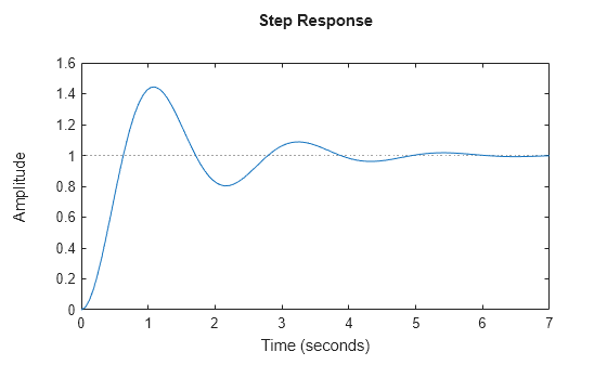
The plot shows the ringdown expected of a second-order system with a low damping ratio.

Discrete-Time MIMO Transfer Function Model

Create a transfer function for the discrete-time, multi-input, multi-output model:

sys(z)=[1z+0.3zz+0.3-z+2z+0.33z+0.3]

with sample time ts = 0.2 seconds.

Specify the numerator coefficients as a 2-by-2 matrix.

numerators = {1 [1 0];[-1 2] 3};

Specify the coefficients of the common denominator as a row vector.

Create the discrete-time MIMO transfer function model.

ts = 0.2;
sys = tf(numerators,denominator,ts)

sys =
 
  From input 1 to output...
          1
   1:  -------
       z + 0.3
 
       -z + 2
   2:  -------
       z + 0.3
 
  From input 2 to output...
          z
   1:  -------
       z + 0.3
 
          3
   2:  -------
       z + 0.3
 
Sample time: 0.2 seconds
Discrete-time transfer function.

For more information on creating MIMO transfer functions, see MIMO Transfer Functions.

Concatenate SISO Transfer Functions into MIMO Transfer Function Model

In this example, you create a MIMO transfer function model by concatenating SISO transfer function models. Consider the following single-input, two-output transfer function:

sys(s)=[s-1s+1s+2s2+4s+5].

Specify the MIMO transfer function model by concatenating the SISO entries.

sys1 = tf([1 -1],[1 1]);		
sys2 = tf([1 2],[1 4 5]);
sys = [sys1;sys2]

sys =
 
  From input to output...
       s - 1
   1:  -----
       s + 1
 
           s + 2
   2:  -------------
       s^2 + 4 s + 5
 
Continuous-time transfer function.

For more information on creating MIMO transfer functions, see MIMO Transfer Functions.

Transfer Function Model Using Rational Expression

For this example, create a continuous-time transfer function model using rational expressions. Using a rational expression can sometimes be easier and more intuitive than specifying polynomial coefficients of the numerator and denominator.

Consider the following system:

sys(s)=ss2+2s+10.

To create the transfer function model, first specify s as a tf object.

s =
 
  s
 
Continuous-time transfer function.

Create the transfer function model using s in the rational expression.

sys =
 
        s
  --------------
  s^2 + 2 s + 10
 
Continuous-time transfer function.

Discrete-Time Transfer Function Model Using Rational Expression

For this example, create a discrete-time transfer function model using a rational expression. Using a rational expression can sometimes be easier and more intuitive than specifying polynomial coefficients.

Consider the following system:

sys(z)=z-1z2-1.85z+0.9.Discrete-time transfer function

To create the transfer function model, first specify z as a tf object and the sample time Ts.

z =
 
  z
 
Sample time: 0.1 seconds
Discrete-time transfer function.

Create the transfer function model using z in the rational expression.

sys = (z - 1) / (z^2 - 1.85*z + 0.9)

sys =
 
        z - 1
  ------------------
  z^2 - 1.85 z + 0.9
 
Sample time: 0.1 seconds
Discrete-time transfer function.

Transfer Function Model with Inherited Properties

For this example, create a transfer function model with properties inherited from another transfer function model. Consider the following two transfer functions:

sys1(s)=2ss2+8sandsys2(s)=s-17s4+2s3+9.

For this example, create sys1 with the TimeUnit and InputDelay property set to ‘minutes‘.

numerator1 = [2,0];
denominator1 = [1,8,0];
sys1 = tf(numerator1,denominator1,'TimeUnit','minutes','InputUnit','minutes')

sys1 =
 
     2 s
  ---------
  s^2 + 8 s
 
Continuous-time transfer function.

propValues1 = [sys1.TimeUnit,sys1.InputUnit]

propValues1 = 1x2 cell
    {'minutes'}    {'minutes'}

Create the second transfer function model with properties inherited from sys1.

numerator2 = [1,-1];
denominator2 = [7,2,0,0,9];
sys2 = tf(numerator2,denominator2,sys1)

sys2 =
 
        s - 1
  -----------------
  7 s^4 + 2 s^3 + 9
 
Continuous-time transfer function.

propValues2 = [sys2.TimeUnit,sys2.InputUnit]

propValues2 = 1x2 cell
    {'minutes'}    {'minutes'}

Observe that the transfer function model sys2 has that same properties as sys1.

Array of Transfer Function Models

You can use a for loop to specify an array of transfer function models.

First, pre-allocate the transfer function array with zeros.

The first two indices represent the number of outputs and inputs for the models, while the third index is the number of models in the array.

Create the transfer function model array using a rational expression in the for loop.

s = tf('s');                                                  
for k = 1:3                                                             
    sys(:,:,k) = k/(s^2+s+k);                                          
end
sys

sys(:,:,1,1) =
 
       1
  -----------
  s^2 + s + 1
 

sys(:,:,2,1) =
 
       2
  -----------
  s^2 + s + 2
 

sys(:,:,3,1) =
 
       3
  -----------
  s^2 + s + 3
 
3x1 array of continuous-time transfer functions.

Convert State-Space Model to Transfer Function

For this example, compute the transfer function of the following state-space model:

A=[-2-11-2],B=[112-1],C=[10],D=[01].

Create the state-space model using the state-space matrices.

A = [-2 -1;1 -2];
B = [1 1;2 -1];
C = [1 0];
D = [0 1];
ltiSys = ss(A,B,C,D);

Convert the state-space model ltiSys to a transfer function.

sys =
 
  From input 1 to output:
        s
  -------------
  s^2 + 4 s + 5
 
  From input 2 to output:
  s^2 + 5 s + 8
  -------------
  s^2 + 4 s + 5
 
Continuous-time transfer function.

Extract Transfer Functions from Identified Model

For this example, extract the measured and noise components of an identified polynomial model into two separate transfer functions.

Load the Box-Jenkins polynomial model ltiSys in identifiedModel.mat.

load('identifiedModel.mat','ltiSys');

ltiSys is an identified discrete-time model of the form: y(t)=BFu(t)+CDe(t), where BF represents the measured component and CD the noise component.

Extract the measured and noise components as transfer functions.

sysMeas = tf(ltiSys,'measured')

sysMeas =
 
  From input "u1" to output "y1":
            -0.1426 z^-1 + 0.1958 z^-2
  z^(-2) * ----------------------------
           1 - 1.575 z^-1 + 0.6115 z^-2
 
Sample time: 0.04 seconds
Discrete-time transfer function.

sysNoise = tf(ltiSys,'noise')

sysNoise =
 
  From input "v@y1" to output "y1":
           0.04556 + 0.03301 z^-1
  ----------------------------------------
  1 - 1.026 z^-1 + 0.26 z^-2 - 0.1949 z^-3
 
Input groups:        
    Name     Channels
    Noise       1    
                     
Sample time: 0.04 seconds
Discrete-time transfer function.

The measured component can serve as a plant model, while the noise component can be used as a disturbance model for control system design.

Specify Input and Output Names for MIMO Transfer Function Model

Transfer function model objects include model data that helps you keep track of what the model represents. For instance, you can assign names to the inputs and outputs of your model.

Consider the following continuous-time MIMO transfer function model:

sys(s)=[s+1s2+2s+21s]

The model has one input — Current, and two outputs — Torque and Angular velocity.

First, specify the numerator and denominator coefficients of the model.

numerators = {[1 1] ; 1};
denominators = {[1 2 2] ; [1 0]};

Create the transfer function model, specifying the input name and output names.

sys = tf(numerators,denominators,'InputName','Current',...
        'OutputName',{'Torque' 'Angular Velocity'})

sys =
 
  From input "Current" to output...
                s + 1
   Torque:  -------------
            s^2 + 2 s + 2
 
                      1
   Angular Velocity:  -
                      s
 
Continuous-time transfer function.

Specify Polynomial Ordering in Discrete-Time Transfer Function

For this example, specify polynomial ordering in discrete-time transfer function models using the ‘Variable‘ property.

Consider the following discrete-time transfer functions with sample time 0.1 seconds:

sys1(z)=z2z2+2z+3sys2(z-1)=11+2z-1+3z-2.

Create the first discrete-time transfer function by specifying the z coefficients.

numerator = [1,0,0];
denominator = [1,2,3];
ts = 0.1;
sys1 = tf(numerator,denominator,ts)

sys1 =
 
       z^2
  -------------
  z^2 + 2 z + 3
 
Sample time: 0.1 seconds
Discrete-time transfer function.

The coefficients of sys1 are ordered in descending powers of z.

tf switches convention based on the value of the ‘Variable‘ property. Since sys2 is the inverse transfer function model of sys1, specify ‘Variable‘ as ‘z^-1‘ and use the same numerator and denominator coefficients.

sys2 = tf(numerator,denominator,ts,'Variable','z^-1')

sys2 =
 
           1
  -------------------
  1 + 2 z^-1 + 3 z^-2
 
Sample time: 0.1 seconds
Discrete-time transfer function.

The coefficients of sys2 are now ordered in ascending powers of z^-1.

Based on different conventions, you can specify polynomial ordering in transfer function models using the ‘Variable‘ property.

Tunable Low-Pass Filter

In this example, you will create a low-pass filter with one tunable parameter a:

F=as+a

Since the numerator and denominator coefficients of a tunableTF block are independent, you cannot use tunableTF to represent F. Instead, construct F using the tunable real parameter object realp.

Create a real tunable parameter with an initial value of 10.

a = 
       Name: 'a'
      Value: 10
    Minimum: -Inf
    Maximum: Inf
       Free: 1

Real scalar parameter.

Use tf to create the tunable low-pass filter F.

numerator = a;
denominator = [1,a];
F = tf(numerator,denominator)

Generalized continuous-time state-space model with 1 outputs, 1 inputs, 1 states, and the following blocks:
  a: Scalar parameter, 2 occurrences.

Type "ss(F)" to see the current value and "F.Blocks" to interact with the blocks.

F is a genss object which has the tunable parameter a in its Blocks property. You can connect F with other tunable or numeric models to create more complex control system models. For an example, see Control System with Tunable Components.

Static Gain MIMO Transfer Function Model

In this example, you will create a static gain MIMO transfer function model.

Consider the following two-input, two-output static gain matrix m:

m=[2435]

Specify the gain matrix and create the static gain transfer function model.

m = [2,4;...
    3,5];
sys1 = tf(m)

sys1 =
 
  From input 1 to output...
   1:  2
 
   2:  3
 
  From input 2 to output...
   1:  4
 
   2:  5
 
Static gain.

You can use static gain transfer function model sys1 obtained above to cascade it with another transfer function model.

For this example, create another two-input, two-output discrete transfer function model and use the series function to connect the two models.

numerators = {1,[1,0];[-1,2],3};
denominator = [1,0.3];
ts = 0.2;
sys2 = tf(numerators,denominator,ts)

sys2 =
 
  From input 1 to output...
          1
   1:  -------
       z + 0.3
 
       -z + 2
   2:  -------
       z + 0.3
 
  From input 2 to output...
          z
   1:  -------
       z + 0.3
 
          3
   2:  -------
       z + 0.3
 
Sample time: 0.2 seconds
Discrete-time transfer function.

sys =
 
  From input 1 to output...
       3 z^2 + 2.9 z + 0.6
   1:  -------------------
       z^2 + 0.6 z + 0.09
 
       -2 z^2 + 12.4 z + 3.9
   2:  ---------------------
        z^2 + 0.6 z + 0.09
 
  From input 2 to output...
       5 z^2 + 5.5 z + 1.2
   1:  -------------------
       z^2 + 0.6 z + 0.09
 
       -4 z^2 + 21.8 z + 6.9
   2:  ---------------------
        z^2 + 0.6 z + 0.09
 
Sample time: 0.2 seconds
Discrete-time transfer function.

Limitations

Transfer function models are ill-suited for numerical computations. Once
created, convert them to state-space form before combining them with other
models or performing model transformations. You can then convert the resulting
models back to transfer function form for inspection purposes
An identified nonlinear model cannot be directly converted into a transfer
function model using tf. To obtain a transfer function model:
1. Convert the nonlinear identified model to an identified LTI model
  using linapp (System Identification Toolbox), idnlarx/linearize (System Identification Toolbox), or
  idnlhw/linearize (System Identification Toolbox).
2. Then, convert the resulting model to a transfer function model
  using tf.

Version History

Introduced before R2006a

Источник

На основе передаточных функций

Использование команд языка сценариев

В среде MatLabсуществует
несколько возможностей задания
передаточных функций линейных систем
управления. В случае работы с помощью
командной строки либо файла сценария
наиболее рационально использовать
функциюtf(transferfunction).

Синтаксис
функции ft:

f=tf(num,den),
где num – коэффициенты полинома
числителя передаточной функции, идущие
по убыванию степени s, аden– коэффициенты полинома знаменателя
передаточной функции, идущие по убыванию
степениs.

Например, передаточная функция

(17)

вводится следующим образом:

>>
n = [2 4]

n
=

2
4

>>
d = [1 1.5 1.5 1]

d
=

1.0000
1.5000 1.5000 1.0000

>>
f = tf ( n, d )

Transfer
function:

2
s + 4

————————-

s^3
+ 1.5 s^2 + 1.5 s + 1

Еще один способ задания передаточной
функции (17):

>>
f = tf ( [2 4], [1 1.5 1.5 1] );

Функции для получения временных
характеристик на основе передаточных
функций приведены в табл. 4.

Таблица 4

Функции для представления временных
характеристик

Функция	Описание функции
step(f) step(f, t)	Вывод в виде графика переходной характеристики системы
impulse(f) impulse(f, t)	Вывод в виде графика импульсной характеристики системы
Примечание. f – передаточная функция; t – интервал времени, для которого будет рассчитан переходный процесс

Использование Simulink

Еще одним способом задания систем в
виде передаточных функций является
использование пакета Simulink,
входящего в составMatLab.

Для представления передаточной функции
в Simulink используется блок Transfer Fcn. Блок
передаточной характеристики Transfer Fcn
задает передаточную функцию в виде
отношения полиномов

, (18)

где nn и nd – порядок числителя и знаменателя
передаточной функции, порядок числителя
не должен превышать порядок знаменателя,
num – вектор или матрица коэффициентов
числителя, den – вектор коэффициентов
знаменателя. Параметры блока TransferFcn:

Numerator
– вектор или матрица коэффициентов
полинома числителя.
Denominator
– вектор коэффициентов полинома
знаменателя.
Absolute
tolerance – абсолютная погрешность.

Исследование переходных характеристик
осуществляется путем подачи на вход
блока, представляющего передаточную
функцию (блок Transfer Fcn), единичного
ступенчатого сигнала (блоки ConstantилиStep). Входной сигнал
блока должен быть скалярным. Чтобы
получить переходный процесс, необходимо
поместить на схему блокScopeи соединить его вход с выходом блока,
переходный процесс которого необходимо
получить. На рис. 6. показан пример
моделирования колебательного звена с
помощью блока Transfer Fcn (схема вSimulinkи переходные процессы, полученные в
блокеScope). Начальные
условия при использовании блока Transfer
Fcn полагаются нулевыми.

Рис.
6. Пример моделирования колебательного
звена с помощью Simulink

2.5. Использование SciLab для моделирования систем
На основе передаточных функций

Использование script-языка

При использовании script-языка SciLab для
представления линейных систем используется
функция syslin.

Синтаксис:

sl
= syslin(dom, N, D)

sl
= syslin(dom, H)

Параметры функции syslin:

dom –
символьная переменная, которая может
принимать два значения: ‘c’ или ‘d’. dom
определяет временной домен системы и
может принимать следующие значения:
dom=’c’ для систем непрерывных во времени;
dom=’d’ для дискретно-временных систем;

N, D –
полиномиальные матрицы;

H –
рациональная матрица;

Выражение s = poly(0,’s’) задаёт полином,
соответствующий оператору Лапласа;
переменная s может быть использована в
дальнейшем. Наряду с таким заданием
можно использовать и константу %s.

Далее приведены альтернативные способы
задания двух ПФ
и.

Пример 1:

s
= poly(0, ‘s’);

H1
=(1+2*s)/s^2

W1
= syslin(‘c’, H1)

H2
= (1+2*s+s^2)/s^2

W2
= syslin(‘c’, H2)

Пример 2:

s
= poly(0, ‘s’);

W1
= syslin(‘c’, 1+2*s, s^2)

W2
= syslin(‘c’, 1+2*s+s^2, s^2)

Пример 3:

W1
= syslin(‘c’, 1+2*%s, %s^2)

W2
= syslin(‘c’, 1+2*%s+%s^2, %s^2)

Для исследования временных характеристик
используется функция csim, предназначенная
для моделирования линейной системы

[y
[,x]] = csim(u, t, sl),

где u –
функция управления, принимает значения
‘step’ или ‘impulse’
в зависимости от вызываемой временной
характеристики;

t – действительный вектор, характеризующий
время; t(1) – начальное время x0=x(t(1));

sl – передаточная функция, представленная
функцией syslin.

Далее рассмотрим в качестве примера
моделирование апериодических звеньев
первого порядка с различными значениями
постоянных времени. Результат моделирования
в виде переходных характеристик приведен
на рис. 7.

Пример:

//
построение переходных характеристик

//
апериодического звена 1-го порядка

K
= 1; // коэффициент усиления

T1
= 0.1; // постоянные времени

T2
= 0.5;

T3
= 1;

W1
= syslin(‘c’, K/(T1*%s + 1));// задать ПФ

W2
= syslin(‘c’, K/(T2*%s + 1));

W3
= syslin(‘c’, K/(T3*%s + 1));

t
= 0:0.05:5; // временной интервал

h1
= csim(‘step’, t, W1); // моделирование подачи

h2
= csim(‘step’, t, W2); // на вход ПФ

h3
= csim(‘step’, t, W3); // ступенчатого воздействия

//
построение графиков

plot(t,
h1, ‘r’, t, h2, ‘g’, t, h3, ‘b’);

xgrid(2);
// установка сетки на графике

//
установка подписей графика и осей

xtitle(‘h(t)’,
‘time, c’, ‘h(t)’);

legend(‘T=0.1’,
‘T=0.5’, ‘T=1’); // подпись легенды

Рис.
7. Переходные
характеристики апериодических звеньев
в SciLab

Соседние файлы в предмете [НЕСОРТИРОВАННОЕ]

Источник

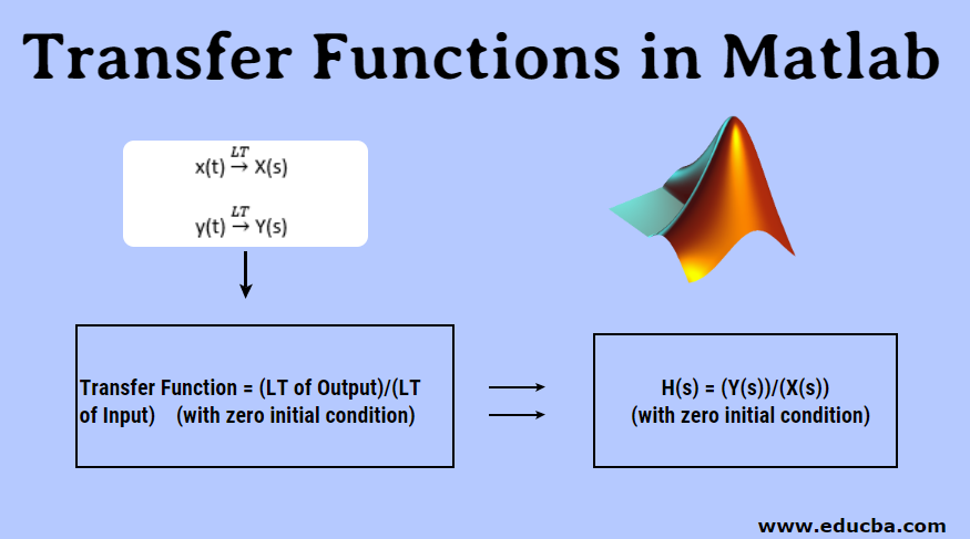
Introduction to Transfer Functions in Matlab

A transfer function is represented by ‘H(s)’. H(s) is a complex function and ‘s’ is a complex variable. It is obtained by taking the Laplace transform of impulse response h(t). transfer function and impulse response are only used in LTI systems. LTI system means Linear and Time invariant system, according to the linear property as the input is zero then output also becomes zero. Therefore if we do not consider initial conditions are zero then linear property will fail and if the property fails then the system will become non-linear. Because of non-linearity system will become Non-LTI system. And for non-LTI system we cannot define transfer function, therefore, it is mandatory to assume initial conditions are zero.

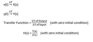
Definition of Transfer Functions in Matlab

The transfer function of the LTI system is the ratio of the Laplace transform of output to the Laplace transform of input of the system by assuming all the initial conditions are zero.

In the above system, the input is x (t) and the output is y(t). After taking Laplace Transform of the whole system, x(t) becomes X(s), y(t) becomes Y(s) .we consider all the initial conditions are zero because

Methods of Transfer Functions in Matlab

There are three methods to obtain the Transfer function in Matlab:

By Using Equation
By Using Coefficients
By Using Pole Zero gain

Let us consider one example

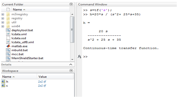
1. By Using Equation

First, we need to declare ‘s’ is a transfer function then type the whole equation in the command window or Matlab editor. In this ‘s’ is the transfer function variable.

Command: “tf”

Syntax : transfer function variable name = tf(‘transfer function variable name’);

Example: s=tf(‘s’);

Matlab program

2. By Using Coefficients

In this method numerator and denominator, coefficients are used followed by ‘tf’ command.

In the above example

The numerator has only one value which is “10s”, so the coefficient is 10.

And in the denominator there are three terms “, so coefficients are 1, 10 and 25.

Command: “tf”

Syntax: transfer function variable name = tf([numerator coefficients ] ,[denominator coefficients])

Example: h= tf([10 0],[1 10 25];

3. By Using Pole Zero gain

In this method, we use the command “zpk”, here z stands for zeros,p stands for poles and k stands for gain.

In above example :

Zeros:

N =0

10 * s =0

(s-0)=0

Here gain is 10 and

s=0

therefore zero present at origin

D= 0

S² + 10s + 25 = 0

S + 5s +5s + 25 = 0

S (s+5) + 5 (s+5) = 0

(s+5)(s+5) = 0

S = -5, -5

Therefore two poles are present at -5.

command: zpk

syntax: zpk([zeros],[poles],gain)

example :zpk([0],[-5 -5],10)

Examples & Syntax of Transfer Functions in Matlab

Below are the various examples of transfer function with their syntax:

Example #1

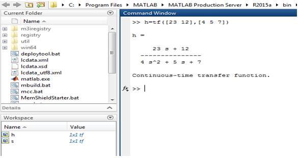
The above example illustrated in screen 1 .in this transfer function represented by using equation as well as ‘tf’ command is used. Values of h and s are stored in the workspace.

Example #2

In this example, the coefficient method is used. Therefore first we need to find out numerator and denominator separately. Here numerator is 23s + 12 and the coefficient of the numerator is 23 and 12. The denominator is and coefficients of the denominator are 4, 5 and 7

The below image shows the Matlab program for the above example.

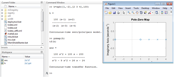
Example #3

In this example input is values of pole, zero, and gain, zpk command is used to find out the transfer function.

Zero’s = 1,-2

Pole’s = 2,3,4

Gain = 100

It shows output

Advantages

Below are some of the advantages explained.

It is a mathematical model that gives Gain of LTI system. mathematical modeling and mathematical equations are useful to understand the performance, characteristics, and stability of the system
Complex integral equations and differential equation converted into the simple algebraic equations (polynomial equations)
The transfer function is dependent on the System and independent on Input.
If the transfer function of the system is known then the output can be easily calculated.
It gives information about poles and zeros, which can be calculated.

Conclusion

In this article, we have studied various methods to represent transfer function in Matlab which are using the equation, using coefficients, and using pole-zero gain information. In Transfer Function representation we can also plot poles, zero plots by using ‘pzmap’ command.

This representation can be obtained in both the ways from equations to pole-zero plot and from pole-zero plot to the equation. Transfer function mostly used in control systems and signals and systems.

Введение в функции передачи в Matlab

Передаточная функция представлена как «H (s)». H (s) — комплексная функция, а s — комплексная переменная. Он получается путем преобразования Лапласа импульсного отклика h (t). Передаточная функция и импульсный отклик используются только в системах LTI. LTI-система означает линейную и инвариантную по времени систему, в соответствии с линейным свойством, поскольку входное значение равно нулю, а выходное значение также становится равным нулю. Следовательно, если мы не считаем начальные условия равными нулю, линейное свойство не будет выполнено, а если свойство не выполнено, то система станет нелинейной. Из-за нелинейности система станет не-LTI системой. А для не-LTI системы мы не можем определить передаточную функцию, поэтому обязательно предположить, что начальные условия равны нулю.

Определение передаточных функций в Matlab

Передаточная функция системы LTI представляет собой отношение преобразования Лапласа на выходе к преобразованию Лапласа на входе системы, предполагая, что все начальные условия равны нулю.

В описанной выше системе входной сигнал равен x (t), а выходной — y (t). После преобразования Лапласа всей системы x (t) становится X (s), y (t) становится Y (s). Мы считаем, что все начальные условия равны нулю, потому что

Методы передаточных функций в Matlab

Существует три способа получения Передаточной функции в Matlab

Используя уравнение
Используя коэффициенты
Используя нулевое усиление полюса

Давайте рассмотрим один пример

1) Используя уравнение

Во-первых, нам нужно объявить ‘s’ как передаточную функцию, а затем ввести полное уравнение в командном окне или редакторе Matlab. В этом ‘s’ является переменной передаточной функции.

Команда: «тф»

Синтаксис : transfer function variable name = tf('transfer function variable name');

Пример: s = tf (‘s’);

Программа Matlab

2) Используя коэффициенты

В этом методе числитель и знаменатель используются коэффициенты, за которыми следует команда «tf».

В приведенном выше примере

Числитель имеет только одно значение, равное 10 с, поэтому коэффициент равен 10.

А в знаменателе есть три термина «, поэтому коэффициенты 1, 10 и 25.

Команда: «тф»

Синтаксис : transfer function variable name = tf((numerator coefficients ), (denominator coefficients))

Пример: h = tf ((10 0), (1 10 25);

3) Используя нулевое усиление полюса

В этом методе мы используем команду «zpk», где z обозначает нули, p обозначает полюсы, а k обозначает усиление.

В приведенном выше примере:

Нули:

N = 0

10 * с = 0

(S-0) = 0

Здесь усиление составляет 10 и

s = 0

следовательно, ноль присутствует в источнике

D = 0

S ² + 10 с + 25 = 0

S + 5s + 5s + 25 = 0

S (s + 5) + 5 (s + 5) = 0

(с + 5) (с + 5) = 0

S = -5, -5

Поэтому два полюса присутствуют в -5.

команда: zpk

синтаксис: zpk ((нули), (полюсы), усиление)

пример: zpk ((0), (- 5 -5), 10)

Примеры и синтаксис передаточных функций в Matlab

Ниже приведены различные примеры передаточной функции с их синтаксисом:

Пример № 1

Вышеприведенный пример, показанный на экране 1, в этой передаточной функции представлен с использованием уравнения, а также команды «tf». Значения h и s хранятся в рабочей области.

Пример № 2

В этом примере используется метод коэффициентов. Поэтому сначала нам нужно выяснить числитель и знаменатель отдельно. Здесь числитель равен 23s + 12, а коэффициент числителя равен 23 и 12. Знаменатель равен, а коэффициенты знаменателя равны 4, 5 и 7.

На рисунке ниже показана программа Matlab для приведенного выше примера.

Пример № 3

В этом примере вводом являются значения полюса, нуля и усиления, команда zpk используется для определения передаточной функции.

Ноль = 1, -2

Полюс = 2, 3, 4

Gain = 100

Показывает вывод

преимущества

Это математическая модель, которая дает усиление системы LTI. математическое моделирование и математические уравнения полезны для понимания производительности, характеристик и стабильности системы
Комплексные интегральные уравнения и дифференциальные уравнения, преобразованные в простые алгебраические уравнения (полиномиальные уравнения)
Передаточная функция зависит от системы и не зависит от входа.
Если передаточная функция системы известна, выход может быть легко рассчитан.
Он дает информацию о полюсах и нулях, может быть рассчитан.

Вывод

В этой статье мы изучили различные методы представления передаточной функции в Matlab, которые используют уравнение, используют коэффициенты и используют информацию об усилении с нулевым полюсом. В представлении передаточной функции мы также можем построить полюсы, нулевой график, используя команду ‘pzmap’.

Это представление может быть получено как из уравнения в график с нулевым полюсом, так и из графика с нулевым полюсом в уравнение. Передаточная функция в основном используется в системах управления, а также в сигналах и системах.

Описание

Используйте tf создать модели передаточной функции с комплексным знаком или с действительным знаком или преобразовать модели динамической системы в форму передаточной функции.

Передаточные функции являются представлением частотного диапазона линейных независимых от времени систем. Например, считайте непрерывное время динамической системой SISO представленный передаточной функцией sys(s) = N(s)/D(s), где s = jw и N(s) и D(s) называются полиномом числителя и полиномом знаменателя, соответственно. tf объект модели может представлять SISO или передаточные функции MIMO в непрерывное время или дискретное время.

Можно создать объект модели передаточной функции или путем определения его коэффициентов непосредственно, или путем преобразования модели другого типа (таких как модель в пространстве состояний ss) к форме передаточной функции. Для получения дополнительной информации смотрите Передаточные функции.

Можно также использовать tf создать обобщенное пространство состояний (genss) модели или неопределенное пространство состояний (uss (Robust Control Toolbox)) модели.

Создание

Синтаксис

Описание

пример

sys = tf(numerator,denominator) создает модель передаточной функции непрерывного времени, устанавливая Numerator и Denominator свойства. Например, считайте непрерывное время динамической системой SISO представленный передаточной функцией sys(s) = N(s)/D(s), входные параметры numerator и denominator коэффициенты N(s) и D(s), соответственно.

пример

sys = tf(numerator,denominator,ts) создает модель передаточной функции дискретного времени, устанавливая Numerator, Denominator, и Ts свойства. Например, считайте дискретное время динамической системой SISO представленный передаточной функцией sys(z) = N(z)/D(z), входные параметры numerator и denominator коэффициенты N(z) и D(z), соответственно. Оставить шаг расчета незаданным, набор ts входной параметр к -1.

пример

sys = tf(numerator,denominator,ltiSys) создает модель передаточной функции со свойствами, наследованными от модели ltiSys динамической системы, включая шаг расчета.

пример

sys = tf(m) создает модель передаточной функции, которая представляет статическое усиление, m.

пример

sys = tf(___,Name,Value) свойства наборов модели передаточной функции, использующей один или несколько Name,Value парные аргументы для любой из предыдущих комбинаций входных аргументов.

пример

sys = tf(ltiSys) преобразует модель ltiSys динамической системы к модели передаточной функции.

пример

sys = tf(ltiSys,component) преобразует заданный component из ltiSys к форме передаточной функции. Используйте этот синтаксис только когда ltiSys идентифицированная модель линейного независимого от времени (LTI).

пример

s = tf('s') создает специальную переменную s то, что можно использовать в рациональном выражении, чтобы создать модель передаточной функции непрерывного времени. Используя рациональное выражение может иногда быть легче и более интуитивным, чем определение полиномиальных коэффициентов.

пример

z = tf('z',ts) создает специальную переменную z то, что можно использовать в рациональном выражении, чтобы создать модель передаточной функции дискретного времени. Оставить шаг расчета незаданным, набор ts входной параметр к -1.

Входные параметры

развернуть все

`numerator` — Коэффициенты числителя передаточной функции
вектор-строка | `Ny`— `Nu` массив ячеек векторов-строк

Коэффициенты числителя передаточной функции в виде:

Вектор-строка из полиномиальных коэффициентов.
Ny— Nu массив ячеек векторов-строк, чтобы задать передаточную функцию MIMO, где Ny количество выходных параметров и Nu количество входных параметров.

Когда вы создаете передаточную функцию, задаете коэффициенты числителя в порядке убывающей степени. Например, если числителем передаточной функции является 3s^2-4s+5, затем задайте numerator как [3 -4 5]. Для передаточной функции дискретного времени с числителем 2z-1, установите numerator к [2 -1].

Также свойство tf объект. Для получения дополнительной информации смотрите Числитель.

`denominator` — Коэффициенты знаменателя передаточной функции
вектор-строка | `Ny`— `Nu` массив ячеек векторов-строк

Коэффициенты знаменателя в виде:

Вектор-строка из полиномиальных коэффициентов.
Ny— Nu массив ячеек векторов-строк, чтобы задать передаточную функцию MIMO, где Ny количество выходных параметров и Nu количество входных параметров.

Когда вы создаете передаточную функцию, задаете коэффициенты знаменателя в порядке убывающей степени. Например, если знаменателем передаточной функции является 7s^2+8s-9, затем задайте denominator как [7 8 -9]. Для передаточной функции дискретного времени со знаменателем 2z^2+1, установите denominator к [2 0 1].

Также свойство tf объект. Для получения дополнительной информации смотрите Знаменатель.

`ts` Размер шага
скаляр

Шаг расчета в виде скаляра. Также свойство tf объект. Для получения дополнительной информации смотрите Ts.

`ltiSys` — Динамическая система
модель динамической системы | массив моделей

Динамическая система в виде SISO или модели динамической системы MIMO или массива моделей динамической системы. Динамические системы, которые можно использовать, включают:

Непрерывное время или дискретное время числовые модели LTI, такие как tf, zpk, ss, или pid модели.
Обобщенные или неопределенные модели LTI такой как genss или uss Модели (Robust Control Toolbox). (Используя неопределенные модели требует программного обеспечения Robust Control Toolbox™.)

Получившаяся передаточная функция принимает
- текущие значения настраиваемых компонентов для настраиваемых блоков системы управления.
- номинальные значения модели для неопределенных блоков системы управления.
Идентифицированные модели LTI, такой как idtf (System Identification Toolbox), idss (System Identification Toolbox), idproc (System Identification Toolbox), idpoly (System Identification Toolbox), и idgrey Модели (System Identification Toolbox). Чтобы выбрать компонент идентифицированной модели, чтобы преобразовать, задайте component. Если вы не задаете component, tf преобразует измеренный компонент идентифицированной модели по умолчанию. (Используя идентифицированные модели требует программного обеспечения System Identification Toolbox™.)

`m` — Статическое усиление
скаляр | матрица

Статическое усиление в виде скаляра или матрицы. Статическое усиление усиления или устойчивого состояния системы представляет отношение выхода к входу при условии устойчивого состояния.

`component` — Компонент идентифицированной модели
`'measured'` (значение по умолчанию) | `'noise'` | `'augmented'`

Компонент идентифицированной модели, чтобы преобразовать в виде одного из следующего:

'measured' — Преобразуйте измеренный компонент sys.
'noise' — Преобразуйте шумовой компонент sys
'augmented' — Преобразуйте и измеренные и шумовые компоненты sys.

component только применяется когда sys идентифицированная модель LTI.

Для получения дополнительной информации об идентифицированных моделях LTI и их измеренных и шумовых компонентах, см. Идентифицированные Модели LTI.

Выходные аргументы

развернуть все

`sys` — Выведите системную модель
`tf` объект модели | `genss` объект модели | `uss` объект модели

Выведите системную модель, возвращенную как:

Передаточная функция (tf) объект модели, когда numerator и denominator входные параметры являются числовыми массивами.
Обобщенная модель в пространстве состояний (genss) объект, когда numerator или denominator входные параметры включают настраиваемые параметры, такой как realp параметры или обобщенные матрицы (genmat). Для примера смотрите Настраиваемый Фильтр Lowpass.
Неопределенная модель в пространстве состояний (uss) объект, когда numerator или denominator входные параметры включают неопределенные параметры. Используя неопределенные модели требует программного обеспечения Robust Control Toolbox. Для примера смотрите Передаточную функцию с Неопределенными Коэффициентами (Robust Control Toolbox).

Свойства

развернуть все

`Numerator` — Коэффициенты числителя
вектор-строка | `Ny`— `Nu` массив ячеек векторов-строк

Коэффициенты числителя в виде:

Вектор-строка из полиномиальных коэффициентов в порядке убывающей степени (для Variable значения 's'ZP, или 'q') или в порядке возрастающей степени (для Variable значения 'z^-1' или 'q^-1').
Ny— Nu массив ячеек векторов-строк, чтобы задать передаточную функцию MIMO, где Ny количество выходных параметров и Nu количество входных параметров. Каждый элемент массива ячеек задает коэффициенты числителя для данной пары ввода/вывода. Если вы задаете оба Numerator и Denominator как массивы ячеек, у них должны быть те же размерности.

Коэффициенты Numerator может быть или с действительным знаком или с комплексным знаком.

`Denominator` — Коэффициенты знаменателя
вектор-строка | `Ny`— `Nu` массив ячеек векторов-строк

Коэффициенты знаменателя в виде:

Вектор-строка из полиномиальных коэффициентов в порядке убывающей степени (для значений Variable значения 's'ZP, или 'q') или в порядке возрастающей степени (для Variable значения 'z^-1' или 'q^-1').
Ny— Nu массив ячеек векторов-строк, чтобы задать передаточную функцию MIMO, где Ny количество выходных параметров и Nu количество входных параметров. Каждый элемент массива ячеек указывает, что коэффициенты числителя для данного вводят / выходная пара. Если вы задаете оба Numerator и Denominator как массивы ячеек, у них должны быть те же размерности.

Если все записи SISO передаточной функции MIMO имеют тот же знаменатель, можно задать Denominator как вектор-строка при определении Numerator как массив ячеек.

Коэффициенты Denominator может быть или с действительным знаком или с комплексным знаком.

`Variable` — Переменная отображения передаточной функции
`'s'` (значение по умолчанию) | `'z'` | `'p'` | `'q'` | `'z^-1'` | `'q^-1'`

Переменная отображения передаточной функции в виде одного из следующего:

's' — Значение по умолчанию для моделей непрерывного времени
'z' — Значение по умолчанию для моделей дискретного времени
'p' — Эквивалентный 's'
'q' — Эквивалентный 'z'
'z^-1' — Инверсия 'z'
'q^-1' — Эквивалентный 'z^-1'

Значение Variable отражается в отображении, и также влияет на интерпретацию Numerator и Denominator векторы коэффициентов для моделей дискретного времени.

Для Variable значения 's'ZP, или 'q', коэффициенты упорядочены в убывающих степенях переменной. Например, считайте вектор-строку [ak ... a1 a0]. Полиномиальный порядок задан как akzk+…+a1z+a0.
Для Variable значения 'z^-1' или 'q^-1', коэффициенты упорядочены в возрастающих степенях переменной. Например, считайте вектор-строку [b0 b1 ... bk]. Полиномиальный порядок задан как b0+b1z−1+…+bkz−k.

Для примеров смотрите, Задают Упорядоченное расположение Полинома в Передаточной функции Дискретного времени, Модели Передаточной функции Используя Рациональное выражение и Модели Передаточной функции Дискретного времени Используя Рациональное выражение.

`IODelay` — Транспортная задержка
0 (значение по умолчанию) | скаляр | `Ny`— `Nu` массив

Транспортная задержка в виде одного из следующего:

Скаляр — Задает транспортную задержку системы SISO или ту же транспортную задержку всех пар ввода/вывода системы MIMO.
Ny— Nu массив — Задает отдельные транспортные задержки каждой пары ввода/вывода системы MIMO. Здесь, Ny количество выходных параметров и Nu количество входных параметров.

Для систем непрерывного времени задайте транспортные задержки единицы измерения времени, заданной TimeUnit свойство. Для систем дискретного времени задайте транспортные задержки целочисленных множителей шага расчета, Ts.

`InputDelay` — Введите задержку
0 (значение по умолчанию) | скаляр | `Nu`— 1 вектор

Введите задержку каждого входного канала в виде одного из следующего:

Скаляр — Задает входную задержку системы SISO или ту же задержку всех входных параметров мультивходной системы.
Nu— 1 вектор — Задают отдельные входные задержки входа мультивходной системы, где Nu количество входных параметров.

Для систем непрерывного времени задайте входные задержки единицы измерения времени, заданной TimeUnit свойство. Для систем дискретного времени задайте входные задержки целочисленных множителей шага расчета, Ts.

Для получения дополнительной информации смотрите Задержки Линейных систем.

`OutputDelay` — Выведите задержку
0 (значение по умолчанию) | скаляр | `Ny`— 1 вектор

Выведите задержку каждого выходного канала в виде одного из следующего:

Скаляр — Задает выходную задержку системы SISO или ту же задержку всех выходных параметров мультивыходной системы.
Ny— 1 вектор — Задают отдельные выходные задержки выхода мультивыходной системы, где Ny количество выходных параметров.

Для систем непрерывного времени задайте выходные задержки единицы измерения времени, заданной TimeUnit свойство. Для систем дискретного времени задайте выходные задержки целочисленных множителей шага расчета, Ts.

Для получения дополнительной информации смотрите Задержки Линейных систем.

`Ts` Размер шага
0 (значение по умолчанию) | положительная скалярная величина | `-1`

Шаг расчета в виде:

0 для систем непрерывного времени.
Положительная скалярная величина, представляющая период выборки системы дискретного времени. Задайте Ts в единице измерения времени, заданной TimeUnit свойство.
-1 для системы дискретного времени с незаданным шагом расчета.

Примечание

Изменение Ts не дискретизирует или передискретизирует модель. Чтобы преобразовать между представлениями непрерывного времени и дискретного времени, использовать c2d и d2c. Чтобы изменить шаг расчета системы дискретного времени, использовать d2d.

`TimeUnit` — Модули переменной Time
`'seconds'` (значение по умолчанию) | `'nanoseconds'` | `'microseconds'` | `'milliseconds'` | `'minutes'` | `'hours'` | `'days'` | `'weeks'` | `'months'` | `'years'` | …

Модули переменной Time в виде одного из следующего:

'nanoseconds'
'microseconds'
'milliseconds'
'seconds'
'minutes'
'hours'
'days'
'weeks'
'months'
'years'

Изменение TimeUnit не оказывает влияния на другие свойства, но изменяет полное поведение системы. Использование chgTimeUnit преобразовывать между единицами измерения времени, не изменяя поведение системы.

`InputName` — Введите названия канала
`''` (значение по умолчанию) | вектор символов | массив ячеек из символьных векторов

Введите названия канала в виде одного из следующего:

Вектор символов, для моделей одно входа.
Массив ячеек из символьных векторов, для мультивходных моделей.
'', никакие заданные имена, для любых входных каналов.

В качестве альтернативы можно присвоить входные имена для мультивходных моделей с помощью автоматического векторного расширения. Например, если sys 2D входная модель, введите следующее:

sys.InputName = 'controls';

Входные имена автоматически расширяются до {'controls(1)';'controls(2)'}.

Можно использовать краткое обозначение u относиться к InputName свойство. Например, sys.u эквивалентно sys.InputName.

Используйте InputName к:

Идентифицируйте каналы на отображении модели и графиках.
Извлеките подсистемы систем MIMO.
Задайте точки контакта когда взаимосвязанные модели.

`InputUnit` — Введите модули канала
`''` (значение по умолчанию) | вектор символов | массив ячеек из символьных векторов

Введите модули канала в виде одного из следующего:

Вектор символов, для моделей одно входа.
Массив ячеек из символьных векторов, для мультивходных моделей.
'', никакие заданные модули, для любых входных каналов.

Используйте InputUnit задавать модули входного сигнала. InputUnit не оказывает влияния на поведение системы.

`InputGroup` — Введите группы канала
структура

Введите группы канала в виде структуры. Используйте InputGroup присваивать входные каналы систем MIMO в группы и относиться к каждой группе по наименованию. Имена полей InputGroup названия группы, и значения полей являются входными каналами каждой группы. Например, введите следующее, чтобы создать входные группы под названием controls и noise это включает входные каналы 1 и 2, и 3 и 5, соответственно.

sys.InputGroup.controls = [1 2];
sys.InputGroup.noise = [3 5];

Можно затем извлечь подсистему из controls входные параметры ко всем выходным параметрам с помощью следующего.

По умолчанию, InputGroup структура без полей.

`OutputName` — Выведите названия канала
`''` (значение по умолчанию) | вектор символов | массив ячеек из символьных векторов

Выведите названия канала в виде одного из следующего:

Вектор символов, для моделей одно выхода.
Массив ячеек из символьных векторов, для мультивыходных моделей.
'', никакие заданные имена, для любых выходных каналов.

В качестве альтернативы можно присвоить выходные имена для мультивыходных моделей с помощью автоматического векторного расширения. Например, если sys 2D выходная модель, введите следующее.

sys.OutputName = 'measurements';

Выходные имена автоматически расширяются до {'measurements(1)';'measurements(2)'}.

Можно также использовать краткое обозначение y относиться к OutputName свойство. Например, sys.y эквивалентно sys.OutputName.

Используйте OutputName к:

Идентифицируйте каналы на отображении модели и графиках.
Извлеките подсистемы систем MIMO.
Задайте точки контакта когда взаимосвязанные модели.

`OutputUnit` — Выведите модули канала
`''` (значение по умолчанию) | вектор символов | массив ячеек из символьных векторов

Выведите модули канала в виде одного из следующего:

Вектор символов, для моделей одно выхода.
Массив ячеек из символьных векторов, для мультивыходных моделей.
'', никакие заданные модули, для любых выходных каналов.

Используйте OutputUnit задавать модули выходного сигнала. OutputUnit не оказывает влияния на поведение системы.

`OutputGroup` — Выведите группы канала
структура

Выведите группы канала в виде структуры. Используйте OutputGroupприсваивать выходные каналы систем MIMO в группы и относиться к каждой группе по наименованию. Имена полей OutputGroup названия группы, и значения полей являются выходными каналами каждой группы. Например, создайте выходные группы под названием temperature и measurement это включает выходные каналы 1, и 3 и 5, соответственно.

sys.OutputGroup.temperature = [1];
sys.InputGroup.measurement = [3 5];

Можно затем извлечь подсистему от всех входных параметров до measurement выходные параметры с помощью следующего.

По умолчанию, OutputGroup структура без полей.

`Name` — Имя системы
`''` (значение по умолчанию) | вектор символов

Имя системы в виде вектора символов. Например, 'system_1'.

`Notes` — Заданный пользователями текст
`{}` (значение по умолчанию) | вектор символов | массив ячеек из символьных векторов

Заданный пользователями текст, который вы хотите сопоставить с системой в виде вектора символов или массива ячеек из символьных векторов. Например, 'System is MIMO'.

`UserData` — Заданные пользователями данные
`[]` (значение по умолчанию) | любой MATLAB^® тип данных

Заданные пользователями данные, которые вы хотите сопоставить с системой в виде любого типа данных MATLAB.

`SamplingGrid` — Выборка сетки для массивов моделей
массив структур

Выборка сетки для массивов моделей в виде массива структур.

Используйте SamplingGrid отслеживать значения переменных, сопоставленные с каждой моделью в массиве моделей, включая идентифицированные линейные независимые от времени массивы моделей (IDLTI).

Установите имена полей структуры к именам переменных выборки. Установите значения полей к произведенным значениям переменных, сопоставленным с каждой моделью в массиве. Все переменные выборки должны быть числовыми скалярами, и все массивы произведенных значений должны совпадать с размерностями массива моделей.

Например, можно создать 11 1 массив линейных моделей, sysarr, путем взятия снимков состояния линейной изменяющейся во времени системы во времена t = 0:10. Следующий код хранит выборки времени линейными моделями.

 sysarr.SamplingGrid = struct('time',0:10)

Точно так же можно создать 6 9 массив моделей, M, путем независимой выборки двух переменных, zeta и w. Следующие кодированные карты (zeta,w) значения к M.

[zeta,w] = ndgrid(<6 values of zeta>,<9 values of w>)
M.SamplingGrid = struct('zeta',zeta,'w',w)

Когда вы отображаете M, каждая запись в массиве включает соответствующий zeta и w значения.

M(:,:,1,1) [zeta=0.3, w=5] =
 
        25
  --------------
  s^2 + 3 s + 25
 

M(:,:,2,1) [zeta=0.35, w=5] =
 
         25
  ----------------
  s^2 + 3.5 s + 25
 
...

Для массивов моделей, сгенерированных путем линеаризации Simulink^® модель в нескольких значениях параметров или рабочих точках, программное обеспечение заполняет SamplingGrid автоматически со значениями переменных, которые соответствуют каждой записи в массиве. Например, команды Simulink Control Design™ linearize (Simulink Control Design) и slLinearizer (Simulink Control Design) заполняет SamplingGrid автоматически.

По умолчанию, SamplingGrid структура без полей.

Функции объекта

Следующие списки содержат представительное подмножество функций, которые можно использовать с tf модели. В общем случае любая функция, применимая к Моделям Динамической системы, применима к tf объект.

развернуть все

Линейный анализ

`step`	Переходный процесс динамической системы; данные о переходном процессе
`impulse`	График импульсной характеристики динамической системы; данные об импульсной характеристике
`lsim`	Постройте диаграмму полюсов-нулей для пар ввода-вывода модели; данные смоделированной реакции системы
`bode`	Диаграмма Боде частотной характеристики, или данные об амплитуде и фазе
`nyquist`	Годограф Найквиста частотной характеристики
`nichols`	График Николса частотной характеристики
`bandwidth`	Полоса пропускания частотной характеристики

Анализ устойчивости

`pole`	Полюса динамической системы
`zero`	Нули и усиление динамической системы SISO
`pzplot`	Диаграмма нулей и полюсов модели динамической системы с дополнительными опциями настройки графика
`margin`	Запас по амплитуде, запас по фазе и частоты среза

Преобразование моделей

`zpk`	Модель нулей, полюсов и усиления
`ss`	Модель в пространстве состояний
`c2d`	Преобразуйте модель от непрерывного до дискретного времени
`d2c`	Преобразуйте модель от дискретного до непрерывного времени
`d2d`	Передискретизируйте дискретную модель

Соединение моделей

`feedback`	Cоединение обратной связи многих моделей
`connect`	Соединения блок-схемы динамических систем
`series`	Последовательная связь двух моделей
`parallel`	Параллельная связь двух моделей

Проектирование контроллера

`pidtune`	Алгоритм настройки ПИДа для линейной модели объекта управления
`rlocus`	График корневого годографа динамической системы
`lqr`	Проект Линейно-квадратичного регулятора (LQR)
`lqg`	Проект «линейного квадратичного гауссова» (LQG)
`lqi`	Линейно-квадратично-интегральное управление
`kalman`	Спроектируйте Фильтр Калмана для оценки состояния

Примеры

свернуть все

Модель передаточной функции SISO

В данном примере рассмотрите следующую модель передаточной функции SISO:

sys(s)=12s2+3s+4.

Задайте числитель и коэффициенты знаменателя, упорядоченные в убывающих степенях s, и создайте модель передаточной функции.

numerator = 1;
denominator = [2,3,4];
sys = tf(numerator,denominator)

sys =
 
         1
  ---------------
  2 s^2 + 3 s + 4
 
Continuous-time transfer function.

Дискретное время модель передаточной функции SISO

В данном примере считайте следующее дискретное время моделью передаточной функции SISO:

sys(z)=2z4z3+3z-1.

Задайте числитель и коэффициенты знаменателя, упорядоченные в убывающих степенях z и шаг расчета 0,1 секунд. Создайте модель передаточной функции дискретного времени.

numerator = [2,0];
denominator = [4,0,3,-1];
ts = 0.1;
sys = tf(numerator,denominator,ts)

sys =
 
        2 z
  ---------------
  4 z^3 + 3 z - 1
 
Sample time: 0.1 seconds
Discrete-time transfer function.

Передаточная функция второго порядка от коэффициента затухания и собственной частоты

В данном примере рассмотрите модель передаточной функции, которая представляет систему второго порядка известной собственной частотой и коэффициентом затухания.

Передаточная функция системы второго порядка, описанной в терминах ее коэффициента затухания ζ и собственная частота ω0:

sys(s)=ω02s2+2ζω0s+ω02.

Принятие коэффициента затухания, ζ = 0.25 и собственная частота, ω0 = 3 рад/с, создайте передаточную функцию второго порядка.

zeta = 0.25;
w0 = 3;
numerator = w0^2;
denominator = [1,2*zeta*w0,w0^2];
sys = tf(numerator,denominator)

sys =
 
         9
  ---------------
  s^2 + 1.5 s + 9
 
Continuous-time transfer function.

Исследуйте ответ этой передаточной функции к входу шага.

График показывает ringdown, ожидаемый системы второго порядка с низким коэффициентом затухания.

Дискретное время модель передаточной функции MIMO

Создайте передаточную функцию в течение дискретного времени, мультивведите, мультивыведите модель:

sys(z)=[1z+0.3zz+0.3-z+2z+0.33z+0.3]

с шагом расчета ts = 0.2 секунды.

Задайте коэффициенты числителя как матрицу 2 на 2.

numerators = {1 [1 0];[-1 2] 3};

Задайте коэффициенты общего знаменателя как вектор-строка.

Создайте дискретное время модель передаточной функции MIMO.

ts = 0.2;
sys = tf(numerators,denominator,ts)

sys =
 
  From input 1 to output...
          1
   1:  -------
       z + 0.3
 
       -z + 2
   2:  -------
       z + 0.3
 
  From input 2 to output...
          z
   1:  -------
       z + 0.3
 
          3
   2:  -------
       z + 0.3
 
Sample time: 0.2 seconds
Discrete-time transfer function.

Для получения дополнительной информации о создании передаточных функций MIMO смотрите Передаточные функции MIMO.

Конкатенация передаточных функций SISO в модель передаточной функции MIMO

В этом примере вы создаете модель передаточной функции MIMO путем конкатенации моделей передаточной функции SISO. Рассмотрите следующий одно вход, 2D выходную передаточную функцию:

sys(s)=[s-1s+1s+2s2+4s+5].

Задайте модель передаточной функции MIMO путем конкатенации записей SISO.

sys1 = tf([1 -1],[1 1]);		
sys2 = tf([1 2],[1 4 5]);
sys = [sys1;sys2]

sys =
 
  From input to output...
       s - 1
   1:  -----
       s + 1
 
           s + 2
   2:  -------------
       s^2 + 4 s + 5
 
Continuous-time transfer function.

Модель передаточной функции Используя рациональное выражение

В данном примере создайте модель передаточной функции непрерывного времени, использующую рациональные выражения. Используя рациональное выражение может иногда быть легче и более интуитивным, чем определение полиномиальных коэффициентов числителя и знаменателя.

Рассмотрите следующую систему:

sys(s)=ss2+2s+10.

Чтобы создать модель передаточной функции, сначала задайте s как tf объект.

s =
 
  s
 
Continuous-time transfer function.

Создайте модель передаточной функции, использующую s в рациональном выражении.

sys =
 
        s
  --------------
  s^2 + 2 s + 10
 
Continuous-time transfer function.

Модель передаточной функции дискретного времени Используя рациональное выражение

В данном примере создайте модель передаточной функции дискретного времени использование рационального выражения. Используя рациональное выражение может иногда быть легче и более интуитивным, чем определение полиномиальных коэффициентов.

Рассмотрите следующую систему:

sys(z)=z-1z2-1.85z+0.9.Передаточная функция дискретного времени

Чтобы создать модель передаточной функции, сначала задайте z как tf возразите и шаг расчета Ts.

z =
 
  z
 
Sample time: 0.1 seconds
Discrete-time transfer function.

Создайте модель передаточной функции использование z в рациональном выражении.

sys = (z - 1) / (z^2 - 1.85*z + 0.9)

sys =
 
        z - 1
  ------------------
  z^2 - 1.85 z + 0.9
 
Sample time: 0.1 seconds
Discrete-time transfer function.

Модель передаточной функции с унаследованными свойствами

В данном примере создайте модель передаточной функции со свойствами, наследованными от другой модели передаточной функции. Рассмотрите следующие две передаточных функции:

sys1(s)=2ss2+8sandsys2(s)=s-17s4+2s3+9.

В данном примере создайте sys1 с TimeUnit и InputDelay набор свойств к ‘minutes‘.

numerator1 = [2,0];
denominator1 = [1,8,0];
sys1 = tf(numerator1,denominator1,'TimeUnit','minutes','InputUnit','minutes')

sys1 =
 
     2 s
  ---------
  s^2 + 8 s
 
Continuous-time transfer function.

propValues1 = [sys1.TimeUnit,sys1.InputUnit]

propValues1 = 1x2 cell
    {'minutes'}    {'minutes'}

Создайте вторую модель передаточной функции со свойствами, наследованными от sys1.

numerator2 = [1,-1];
denominator2 = [7,2,0,0,9];
sys2 = tf(numerator2,denominator2,sys1)

sys2 =
 
        s - 1
  -----------------
  7 s^4 + 2 s^3 + 9
 
Continuous-time transfer function.

propValues2 = [sys2.TimeUnit,sys2.InputUnit]

propValues2 = 1x2 cell
    {'minutes'}    {'minutes'}

Заметьте что модель sys2 передаточной функции имеет те же самые свойства как sys1.

Массив моделей передаточной функции

Можно использовать for цикл, чтобы задать массив моделей передаточной функции.

Во-первых, предварительно выделите массив передаточной функции с нулями.

Первые два индекса представляют количество выходных параметров и входных параметров для моделей, в то время как третий индекс является количеством моделей в массиве.

Создайте массив моделей передаточной функции с помощью рационального выражения в for цикл.

s = tf('s');                                                  
for k = 1:3                                                             
    sys(:,:,k) = k/(s^2+s+k);                                          
end
sys

sys(:,:,1,1) =
 
       1
  -----------
  s^2 + s + 1
 

sys(:,:,2,1) =
 
       2
  -----------
  s^2 + s + 2
 

sys(:,:,3,1) =
 
       3
  -----------
  s^2 + s + 3
 
3x1 array of continuous-time transfer functions.

Преобразуйте модель в пространстве состояний в передаточную функцию

В данном примере вычислите передаточную функцию следующей модели в пространстве состояний:

A=[-2-11-2],B=[112-1],C=[10],D=[01].

Создайте модель в пространстве состояний с помощью матриц пространства состояний.

A = [-2 -1;1 -2];
B = [1 1;2 -1];
C = [1 0];
D = [0 1];
ltiSys = ss(A,B,C,D);

Преобразуйте модель в пространстве состояний ltiSys к передаточной функции.

sys =
 
  From input 1 to output:
  s + 6.28e-16
  -------------
  s^2 + 4 s + 5
 
  From input 2 to output:
  s^2 + 5 s + 8
  -------------
  s^2 + 4 s + 5
 
Continuous-time transfer function.

Извлеките передаточные функции из идентифицированной модели

В данном примере извлеките измеренные и шумовые компоненты идентифицированной полиномиальной модели в две отдельных передаточных функции.

Загрузите полиномиальную модель Бокса-Дженкинса ltiSys в identifiedModel.mat.

load('identifiedModel.mat','ltiSys');

ltiSys идентифицированная модель дискретного времени формы: y(t)=BFu(t)+CDe(t), где BF представляет измеренный компонент и CD шумовой компонент.

Извлеките измеренные и шумовые компоненты как передаточные функции.

sysMeas = tf(ltiSys,'measured')

sysMeas =
 
  From input "u1" to output "y1":
            -0.1426 z^-1 + 0.1958 z^-2
  z^(-2) * ----------------------------
           1 - 1.575 z^-1 + 0.6115 z^-2
 
Sample time: 0.04 seconds
Discrete-time transfer function.

sysNoise = tf(ltiSys,'noise')

sysNoise =
 
  From input "v@y1" to output "y1":
           0.04556 + 0.03301 z^-1
  ----------------------------------------
  1 - 1.026 z^-1 + 0.26 z^-2 - 0.1949 z^-3
 
Input groups:        
    Name     Channels
    Noise       1    
                     
Sample time: 0.04 seconds
Discrete-time transfer function.

Измеренный компонент может служить моделью объекта управления, в то время как шумовой компонент может использоваться в качестве возмущения для проекта системы управления.

Задайте имена ввода и вывода для модели передаточной функции MIMO

Объекты модели передаточной функции включают данные модели, которые помогают вам отслеживать то, что представляет модель. Например, можно присвоить имена к вводам и выводам модели.

Считайте следующее непрерывное время моделью передаточной функции MIMO:

sys(s)=[s+1s2+2s+21s]

Модель имеет вход того — Текущий, и два выходных параметров — Крутящий момент и Скорость вращения.

Во-первых, задайте числитель и коэффициенты знаменателя модели.

numerators = {[1 1] ; 1};
denominators = {[1 2 2] ; [1 0]};

Создайте модель передаточной функции, задав входное имя и выведите имена.

sys = tf(numerators,denominators,'InputName','Current',...
        'OutputName',{'Torque' 'Angular Velocity'})

sys =
 
  From input "Current" to output...
                s + 1
   Torque:  -------------
            s^2 + 2 s + 2
 
                      1
   Angular Velocity:  -
                      s
 
Continuous-time transfer function.

Задайте упорядоченное расположение полинома в передаточной функции дискретного времени

В данном примере задайте упорядоченное расположение полинома в моделях передаточной функции дискретного времени с помощью ‘VariableСвойство.

Считайте следующие передаточные функции дискретного времени с шагом расчета 0,1 секундами:

sys1(z)=z2z2+2z+3sys2(z-1)=11+2z-1+3z-2.

Создайте первую передаточную функцию дискретного времени путем определения z коэффициенты.

numerator = [1,0,0];
denominator = [1,2,3];
ts = 0.1;
sys1 = tf(numerator,denominator,ts)

sys1 =
 
       z^2
  -------------
  z^2 + 2 z + 3
 
Sample time: 0.1 seconds
Discrete-time transfer function.

Коэффициенты sys1 упорядочены в убывающих степенях z.

tf соглашение переключателей на основе значения ‘VariableСвойство. Начиная с sys2 обратная модель передаточной функции sys1, задайте ‘Variable‘как ‘z^-1‘и используйте тот же числитель и коэффициенты знаменателя.

sys2 = tf(numerator,denominator,ts,'Variable','z^-1')

sys2 =
 
           1
  -------------------
  1 + 2 z^-1 + 3 z^-2
 
Sample time: 0.1 seconds
Discrete-time transfer function.

Коэффициенты sys2 теперь упорядочены в возрастающих степенях z^-1.

На основе различных соглашений можно задать упорядоченное расположение полинома в моделях передаточной функции с помощью ‘VariableСвойство.

Настраиваемый фильтр lowpass

В этом примере вы создадите фильтр lowpass с одним настраиваемым параметром a:

F=as+a

Начиная с числителя и коэффициентов знаменателя tunableTF блок независим, вы не можете использовать tunableTF представлять F. Вместо этого создайте F использование настраиваемого действительного объекта параметра realp.

Создайте действительный настраиваемый параметр с начальным значением 10.

a = 
       Name: 'a'
      Value: 10
    Minimum: -Inf
    Maximum: Inf
       Free: 1

Real scalar parameter.

Используйте tf чтобы создать настраиваемый lowpass фильтруют F.

numerator = a;
denominator = [1,a];
F = tf(numerator,denominator)

F =

  Generalized continuous-time state-space model with 1 outputs, 1 inputs, 1 states, and the following blocks:
    a: Scalar parameter, 2 occurrences.

Type "ss(F)" to see the current value, "get(F)" to see all properties, and "F.Blocks" to interact with the blocks.

F genss объект, который имеет настраиваемый параметр a в его Blocks свойство. Можно соединить F с другими настраиваемыми или числовыми моделями, чтобы создать более комплексные модели системы управления. Для примера смотрите Систему управления с Настраиваемыми Компонентами.

Статическое усиление модель передаточной функции MIMO

В этом примере вы создадите статическое усиление модель передаточной функции MIMO.

Рассмотрите следующий 2D вход, 2D выход статическая матрица усиления m:

m=[2435]

Задайте матрицу усиления и создайте статическую модель передаточной функции усиления.

m = [2,4;...
    3,5];
sys1 = tf(m)

sys1 =
 
  From input 1 to output...
   1:  2
 
   2:  3
 
  From input 2 to output...
   1:  4
 
   2:  5
 
Static gain.

Можно использовать статическую модель sys1 передаточной функции усиления полученный выше, чтобы расположить каскадом его с другой моделью передаточной функции.

В данном примере создайте другой 2D вход, 2D выход дискретная модель передаточной функции и используйте series функционируйте, чтобы соединить эти две модели.

numerators = {1,[1,0];[-1,2],3};
denominator = [1,0.3];
ts = 0.2;
sys2 = tf(numerators,denominator,ts)

sys2 =
 
  From input 1 to output...
          1
   1:  -------
       z + 0.3
 
       -z + 2
   2:  -------
       z + 0.3
 
  From input 2 to output...
          z
   1:  -------
       z + 0.3
 
          3
   2:  -------
       z + 0.3
 
Sample time: 0.2 seconds
Discrete-time transfer function.

sys =
 
  From input 1 to output...
       3 z^2 + 2.9 z + 0.6
   1:  -------------------
       z^2 + 0.6 z + 0.09
 
       -2 z^2 + 12.4 z + 3.9
   2:  ---------------------
        z^2 + 0.6 z + 0.09
 
  From input 2 to output...
       5 z^2 + 5.5 z + 1.2
   1:  -------------------
       z^2 + 0.6 z + 0.09
 
       -4 z^2 + 21.8 z + 6.9
   2:  ---------------------
        z^2 + 0.6 z + 0.09
 
Sample time: 0.2 seconds
Discrete-time transfer function.

Ограничения

Модели передаточной функции являются неподходящими для численных расчетов. После того, как созданный, преобразуйте их в форму пространства состояний прежде, чем объединить их с другими моделями или выполнить преобразования моделей. Можно затем преобразовать получившиеся модели назад в форму передаточной функции в инспекционных целях
Идентифицированная нелинейная модель не может быть непосредственно преобразована в использование модели передаточной функции tf. Получить модель передаточной функции:
1. Преобразуйте нелинейную идентифицированную модель в идентифицированное использование модели LTI linapp (System Identification Toolbox), idnlarx/linearize (System Identification Toolbox), или idnlhw/linearize (System Identification Toolbox).
2. Затем преобразуйте получившуюся модель в модель передаточной функции использование tf.

Представлено до R2006a

Источник

tf

Description

Creation

Syntax

Description

Input Arguments

numerator — Numerator coefficients of the transfer function row vector | Ny-by-Nu cell array of row vectors

denominator — Denominator coefficients of the transfer function row vector | Ny-by-Nu cell array of row vectors

ts — Sample time scalar

ltiSys — Dynamic system dynamic system model | model array

m — Static gain scalar | matrix

component — Component of identified model 'measured' (default) | 'noise' | 'augmented'

Output Arguments

sys — Output system model tf model object | genss model object | uss model object

Properties

Numerator — Numerator coefficients row vector | Ny-by-Nu cell array of row vectors

Denominator — Denominator coefficients row vector | Ny-by-Nu cell array of row vectors

Variable — Transfer function display variable 's' (default) | 'z' | 'p' | 'q' | 'z^-1' | 'q^-1'

IODelay — Transport delay 0 (default) | scalar | Ny-by-Nu array

InputDelay — Input delay 0 (default) | scalar | Nu-by-1 vector

OutputDelay — Output delay 0 (default) | scalar | Ny-by-1 vector

Ts — Sample time 0 (default) | positive scalar | -1

TimeUnit — Time variable units 'seconds' (default) | 'nanoseconds' | 'microseconds' | 'milliseconds' | 'minutes' | 'hours' | 'days' | 'weeks' | 'months' | 'years' | …

InputName — Input channel names '' (default) | character vector | cell array of character vectors

InputUnit — Input channel units '' (default) | character vector | cell array of character vectors

InputGroup — Input channel groups structure

OutputName — Output channel names '' (default) | character vector | cell array of character vectors

OutputUnit — Output channel units '' (default) | character vector | cell array of character vectors

OutputGroup — Output channel groups structure

Name — System name '' (default) | character vector

Notes — User-specified text {} (default) | character vector | cell array of character vectors

UserData — User-specified data [] (default) | any MATLAB® data type

SamplingGrid — Sampling grid for model arrays structure array

Object Functions

Linear Analysis

Stability Analysis

Model Transformation

Model Interconnection

Controller Design

Examples

SISO Transfer Function Model

Discrete-Time SISO Transfer Function Model

Second-Order Transfer Function from Damping Ratio and Natural Frequency

Discrete-Time MIMO Transfer Function Model

Concatenate SISO Transfer Functions into MIMO Transfer Function Model

Transfer Function Model Using Rational Expression

Discrete-Time Transfer Function Model Using Rational Expression

Transfer Function Model with Inherited Properties

Array of Transfer Function Models

Convert State-Space Model to Transfer Function

Extract Transfer Functions from Identified Model

Specify Input and Output Names for MIMO Transfer Function Model

Specify Polynomial Ordering in Discrete-Time Transfer Function

Tunable Low-Pass Filter

Static Gain MIMO Transfer Function Model

Limitations

Version History

На основе передаточных функций

Использование команд языка сценариев

Использование Simulink

2.5. Использование SciLab для моделирования систем

На основе передаточных функций

Использование script-языка

Introduction to Transfer Functions in Matlab

Definition of Transfer Functions in Matlab

Methods of Transfer Functions in Matlab

1. By Using Equation

2. By Using Coefficients

3. By Using Pole Zero gain

Examples & Syntax of Transfer Functions in Matlab

Example #1

Example #2

Example #3

Advantages

Conclusion

Recommended Articles

Введение в функции передачи в Matlab

Определение передаточных функций в Matlab

Методы передаточных функций в Matlab

1) Используя уравнение

`numerator` — Numerator coefficients of the transfer function
row vector | `Ny`-by-`Nu` cell array of row
vectors

`denominator` — Denominator coefficients of the transfer function
row vector | `Ny`-by-`Nu` cell array of row
vectors

`ts` — Sample time
scalar

`ltiSys` — Dynamic system
dynamic system model | model array

`m` — Static gain
scalar | matrix

`component` — Component of identified model
`'measured'` (default) | `'noise'` | `'augmented'`

`sys` — Output system model
`tf` model object | `genss` model object | `uss` model object

`Numerator` — Numerator coefficients
row vector | `Ny`-by-`Nu` cell array of row
vectors

`Denominator` — Denominator coefficients
row vector | `Ny`-by-`Nu` cell array of row
vectors

`Variable` — Transfer function display variable
`'s'` (default) | `'z'` | `'p'` | `'q'` | `'z^-1'` | `'q^-1'`

`IODelay` — Transport delay
`0` (default) | scalar | `Ny`-by-`Nu` array

`InputDelay` — Input delay
`0` (default) | scalar | `Nu`-by-1 vector

`OutputDelay` — Output delay
`0` (default) | scalar | `Ny`-by-1 vector

`Ts` — Sample time
`0` (default) | positive scalar | `-1`

`TimeUnit` — Time variable units
`'seconds'` (default) | `'nanoseconds'` | `'microseconds'` | `'milliseconds'` | `'minutes'` | `'hours'` | `'days'` | `'weeks'` | `'months'` | `'years'` | …

`InputName` — Input channel names
`''` (default) | character vector | cell array of character vectors

`InputUnit` — Input channel units
`''` (default) | character vector | cell array of character vectors

`InputGroup` — Input channel groups
structure

`OutputName` — Output channel names
`''` (default) | character vector | cell array of character vectors

`OutputUnit` — Output channel units
`''` (default) | character vector | cell array of character vectors

`OutputGroup` — Output channel groups
structure

`Name` — System name
`''` (default) | character vector

`Notes` — User-specified text
`{}` (default) | character vector | cell array of character vectors

`UserData` — User-specified data
`[]` (default) | any MATLAB^® data type

`SamplingGrid` — Sampling grid for model arrays
structure array

`numerator` — Коэффициенты числителя передаточной функции
вектор-строка | `Ny`— `Nu` массив ячеек векторов-строк

`denominator` — Коэффициенты знаменателя передаточной функции
вектор-строка | `Ny`— `Nu` массив ячеек векторов-строк

`ts` Размер шага
скаляр

`ltiSys` — Динамическая система
модель динамической системы | массив моделей

`m` — Статическое усиление
скаляр | матрица

`component` — Компонент идентифицированной модели
`'measured'` (значение по умолчанию) | `'noise'` | `'augmented'`

`sys` — Выведите системную модель
`tf` объект модели | `genss` объект модели | `uss` объект модели

`Numerator` — Коэффициенты числителя
вектор-строка | `Ny`— `Nu` массив ячеек векторов-строк

`Denominator` — Коэффициенты знаменателя
вектор-строка | `Ny`— `Nu` массив ячеек векторов-строк

`Variable` — Переменная отображения передаточной функции
`'s'` (значение по умолчанию) | `'z'` | `'p'` | `'q'` | `'z^-1'` | `'q^-1'`

`IODelay` — Транспортная задержка
0 (значение по умолчанию) | скаляр | `Ny`— `Nu` массив

`InputDelay` — Введите задержку
0 (значение по умолчанию) | скаляр | `Nu`— 1 вектор

`OutputDelay` — Выведите задержку
0 (значение по умолчанию) | скаляр | `Ny`— 1 вектор

`Ts` Размер шага
0 (значение по умолчанию) | положительная скалярная величина | `-1`

`TimeUnit` — Модули переменной Time
`'seconds'` (значение по умолчанию) | `'nanoseconds'` | `'microseconds'` | `'milliseconds'` | `'minutes'` | `'hours'` | `'days'` | `'weeks'` | `'months'` | `'years'` | …

`InputName` — Введите названия канала
`''` (значение по умолчанию) | вектор символов | массив ячеек из символьных векторов

`InputUnit` — Введите модули канала
`''` (значение по умолчанию) | вектор символов | массив ячеек из символьных векторов

`InputGroup` — Введите группы канала
структура

`OutputName` — Выведите названия канала
`''` (значение по умолчанию) | вектор символов | массив ячеек из символьных векторов

`OutputUnit` — Выведите модули канала
`''` (значение по умолчанию) | вектор символов | массив ячеек из символьных векторов

`OutputGroup` — Выведите группы канала
структура

`Name` — Имя системы
`''` (значение по умолчанию) | вектор символов

`Notes` — Заданный пользователями текст
`{}` (значение по умолчанию) | вектор символов | массив ячеек из символьных векторов

`UserData` — Заданные пользователями данные
`[]` (значение по умолчанию) | любой MATLAB^® тип данных

`SamplingGrid` — Выборка сетки для массивов моделей
массив структур