Если
функция ![]() имеет
имеет
производную в каждой точке ![]() своей
своей
области определения, то ее производная ![]() есть
есть
функция от ![]() .
.
Функция ![]() ,
,
в свою очередь, может иметь производную,
которую называют производной
второго порядка функции ![]() (или второй
(или второй
производной)
и обозначают символом ![]() .
.
Таким образом
![]()
Пример
Задание. Найти
вторую производную функции ![]()
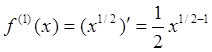
Решение. Для
начала найдем первую производную:
![]()
![]()
![]()
![]()
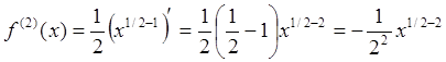
Для
нахождения второй производной
продифференцируем выражение для первой
производной еще раз:
![]()
![]()
![]()
![]()
![]()
![]()
![]()
![]()
Ответ. ![]()
Больше
примеров решенийРешение
производных онлайн
Производные
более высоких порядков определяются
аналогично. То есть производная ![]() -го
-го
порядка функции ![]() есть
есть
первая производная от производной ![]() -го
-го
порядка этой функции:
![]()
Формула Тейлора
Формула
Тейлора показывает
поведение функции в окрестности некоторой
точки. Формула Тейлора функции часто
используется при доказательстве теорем
в дифференциальном исчислении.
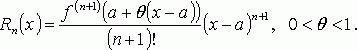
Формула
Тейлора
![]()
,
где Rn(x) —
остаточный член формулы Тейлора.
Остаточный
член формулы Тейлора
В
форме Лагранжа:
В
форме Коши:
![]()
12.Неопределенный
и определенный интегралы
Неопределённый
интеграл.
![]() Определение.
Определение.
Функция F(x) называется первообразной
для функции f(x) на интервале X=(a,b) (конечном
или бесконечном), если в каждой точке
этого интервала f(x) является производной
дляF(x), т.е. ![]() .
.
![]() Из
Из
этого определения следует, что задача
нахождения первообразной обратна задаче
дифференцирования: по заданной функции
f(x ) требуется найти функцию F(x), производная
которой равна f(x).
![]() Первообразная
Первообразная
определена неоднозначно: для
функции ![]() первообразными
первообразными
будут и функция arctg x, и функция arctg
x-10: ![]() .
.
Для того, чтобы описать все множество
первообразных функции f(x), рассмотрим
![]() Свойства
Свойства
первообразной.
-
Если
функция F(x) — первообразная для функции
f(x) на интервале X, то функция f(x) + C, где
C — произвольная постоянная, тоже будет
первообразной для f(x) на этом интервале.
(Док-во: ).
). -
Если
функция F(x) — некоторая первообразная
для функции f(x) на интервале X=(a,b), то
любая другая первообразная F1(x) может
быть представлена в виде F1(x) = F(x) + C, где
C — постоянная на X функция.
![]() Из
Из
этих свойств следует, что если F(x) —
некоторая первообразная функции f(x) на
интервале X, то всё множество первообразных
функции f(x) (т.е. функций, имеющих
производную f(x) и дифференциал f(x) dx) на
этом интервале описывается выражением
F(x) + C, где C — произвольная постоянная.
Неопределённый
интеграл и его свойства.
![]() Определение.
Определение.
Множество первообразных функции f(x)
называется неопределённым интегралом
от этой функции и обозначается
символом ![]() .
.
![]() Как
Как
следует из изложенного выше, если F(x) —
некоторая первообразная функции f(x),
то ![]() ,
,
где C — произвольная постоянная. Функцию
f(x) принято называть подынтегральной
функцией, произведение f(x) dx — подынтегральным
выражением.
![]() Свойства
Свойства
неопределённого интеграла, непосредственно
следующие из определения:
-
 .
. -
 (или
(или  ).
).
Таблица
неопределённых интегралов.
|
1 |
|
11 |
|
|
2 |
|
12 |
|
|
3 |
|
13 |
|
|
4 |
|
14 |
|
|
5 |
|
15 |
|
|
6 |
|
16 |
|
|
7 |
|
17 |
|
|
8 |
|
18 |
|
|
9 |
|
19 |
|
|
10 |
|
20 |
|
В
формулах 14, 15, 16, 19 предполагается, что
a>0. Каждая из формул таблицы справедлива
на любом интервале, на котором непрерывна
подынтегральная функция. Все эти формулы
можно доказать дифференцированием
правой части. Докажем, например, формулу
4: если x > 0, то ![]() ;
;
если x < 0, то ![]() .
.
Простейшие
правила интегрирования.
-
 (
( )
) -

Соседние файлы в предмете [НЕСОРТИРОВАННОЕ]
- #
- #
- #
- #
- #
- #
- #
- #
- #
- #
- #
Идея представления функции в виде многочлена с остаточным слагаемым основана на разложении функции в степенной ряд.
Ряды Тейлора и Маклорена
Бесконечно дифференцируемую в точке x0x_0 функцию действительной переменной f(x)f(x) можно разложить в ряд по степеням двучлена (x−x0)(x-x_0):
f(x)=f(x0)+f′(x0)1!(x−x0)+f′′(x0)2!(x−x0)2+…+f(n)(x0)n!(x−x0)n+…=f(x)=f(x_0)+dfrac{f{‘}(x_0)}{1!}(x-x_0) +dfrac{f{»}(x_0)}{2!}(x-x_0)^2 +ldots+dfrac{f^{(n)}(x_0)}{n!}(x-x_0)^n +ldots =
=∑k=0∞f(k)(x0)k!(x−x0)k=sumlimits_{k=0}^{infty} dfrac{f^{(k)}(x_0)}{k!}(x-x_0)^k
Этот ряд называют рядом Тейлора.
В случае x0=0x_0=0, полученный степенной ряд:
f(x)=f(0)+f′(0)1!x+f′′(0)2!(x−x0)2+…+f(n)(x0)n!(x−x0)n+…=f(x)=f(0)+dfrac{f{‘}( 0)}{1!} x +dfrac{f{»}(0)}{2!}(x-x_0)^2 +ldots+dfrac{f^{(n)}(x_0)}{n!}(x-x_0)^n +ldots =
=∑k=0∞f(k)(x0)k!(x−x0)k=sumlimits_{k=0}^{infty} dfrac{f^{(k)}(x_0)}{k!}(x-x_0)^k
называют рядом Маклорена.
Запишем разложения основных элементарных функций в ряд Маклорена, укажем соответствующие интервалы сходимости и приведем примеры их определения.
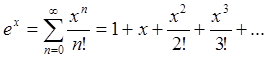
- Показательная функция:
ex=1+x1!+x22!+x33!+…+xnn!+…=∑k=1∞xnn!,∣x∣<∞e^x=1+dfrac{x}{1!} +dfrac{x^2}{2!} +dfrac{x^3}{3!}+ldots+dfrac{x^n}{n!}+ldots=sumlimits_{k=1}^{infty} dfrac{x^n}{n!},quad |x|<infty
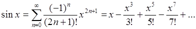
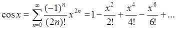
- Тригонометрические функции:
sinx=x1!−x33!+x55!−x77!+…+(−1)n+1x2n−1(2n−1)!+…=∑k=1∞(−1)k+1x2k−1(2k−1)!,∣x∣<∞sin x=dfrac{x}{1!} -dfrac{x^3}{3!} +dfrac{x^5}{5!} -dfrac{x^7}{7!} +ldots+dfrac{(-1)^{n+1}x^{2n-1}}{(2n-1)!}+ldots=sumlimits_{ k =1}^{infty} dfrac{(-1)^{ k +1}x^{2 k -1}}{(2 k -1)!},quad |x|<infty
cosx=1−x22!+x44!−x66!+…+(−1)n+1x2n(2n)!+…=∑k=0∞(−1)kx2k(2k)!,∣x∣<∞cos x=1 -dfrac{x^2}{2!} +dfrac{x^4}{4!} -dfrac{x^6}{6!} +ldots+dfrac{(-1)^{n+1}x^{2n}}{(2n)!}+ldots=sumlimits_{ k =0}^{infty} dfrac{(-1)^{k}x^{2 k }}{(2 k)!},quad |x|<infty
arctgx=x−x33+x55−x77+…+(−1)nx2n+12n+1+…=∑k=0∞(−1)kx2k+12k+1,∣x∣≤1arctg x=x-dfrac{x^3}{3} +dfrac{x^5}{5} -dfrac{x^7}{7} +ldots+dfrac{(-1)^{n}x^{2n+1}}{2n+1}+ldots=sumlimits_{ k =0}^{infty} dfrac{(-1)^{ k }x^{2 k +1}}{2 k +1},quad |x|le{1}
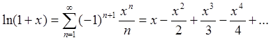
- Логарифмическая функции:
ln(1+x)=x1!−x22!+x33!−x44!+…+(−1)n+1xnn!+…=∑k=1∞(−1)k+1xkk!,x∈(−1;1]ln (1+x)=dfrac{x}{1!} -dfrac{x^2}{2!} +dfrac{x^3}{3!} -dfrac{x^4}{4!} +ldots+dfrac{(-1)^{n+1}x^{n}}{n!}+ldots=sumlimits_{ k =1}^{infty} dfrac{(-1)^{ k +1}x^{ k }}{ k!},quad xin (-1;1]
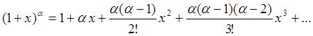
- Степенная функции:
(1+x)α=1+α1!x+α(α−1)2!x2+α(α−1)(α−2)3!x3+…+α(α−1)…(α−n+1)n!xn+…=(1+x)^alpha=1+dfrac{alpha }{1!}x+dfrac{alpha (alpha -1)}{2!}x^2 +dfrac{alpha (alpha -1)( alpha -2)}{3!} x^3 +ldots+dfrac{alpha (alpha -1) ldots ( alpha-n+1)} {n!} {x^n}+ldots=
=∑k=0∞α(α−1)…(α−k+1)k!xk=sumlimits_{ k =0}^{infty} dfrac{alpha (alpha -1) ldots ( alpha-k+1)}{ k!} {x^ k }
11−x=1+x+x2+…+xn+…=∑k=0∞xk,∣x∣<1dfrac{1}{1-x}=1+x+x^2+ldots+x^n+ldots =sumlimits_{ k =0}^{infty}x^{ k },quad |x|<1
Пример 1
Найдем для функции:
f(x)=sinxf(x)=sin x
интервал сходимости ряда:
f(x)=sinx==∑n=1∞(−1)n+1x2n−1(2n−1)!f(x)=sin x==sumlimits_{n=1}^{infty} dfrac{(-1)^{n+1}x^{2n-1}}{(2n-1)!}
Воспользуемся признаком Даламбера:
limn→∞∣an+1an∣=limn→∞∣x2n+1/(2n+1)!x2n−1/(2n−1)!∣=x2limn→∞12n(2n+1)=0limlimits_{n to infty } left | dfrac {a_{n+1}}{a_n} right | = limlimits_{n to infty } left | dfrac {x^{2n+1}/{(2n+1)!}}{ x^{2n-1}/{(2n-1)!}} right | =x^2 limlimits_{n to infty } dfrac {1} {2n(2n+1)}=0
Полученный результат говорит о том, что предел равен нулю для любого xx, и, следовательно, интервалом сходимости ряда является вся числовая ось.
Пример 2
Найдем интервал сходимости ряда для функции
f(x)=arctgx=∑n=0∞(−1)nx2n+12n+1,∣x∣≤1f(x)=arctg x= sumlimits_{n=0}^{infty} dfrac{(-1)^{n}x^{2n+1}}{2n+1}, quad |x|le{1}
Воспользовавшись признаком Даламбера применительно к степенному ряду, получаем:
limn→∞∣an+1an∣=limn→∞∣x2n+1/(2n+1)x2n−1/(2n−1)∣=x2limn→∞2n−12n+1=x2limn→∞2−1n2+1n=x2limlimits_{n to infty } left | dfrac {a_{n+1}}{a_n} right | = limlimits_{n to infty } left | dfrac {x^{2n+1}/(2n+1)}{ x^{2n-1}/(2n-1)} right | =x^2 limlimits_{n to infty } dfrac {2n-1} {2n+1}=x^2 limlimits_{n to infty } dfrac {2-dfrac{1}{n}}{2+dfrac{1}{n}}= x^2
Условие сходимости по этому признаку имеет вид:
x2<1x^2<1
В граничных точках x=±1x=pm1 получаем знакопеременный ряд вида:
∑n=0∞anx2n+1sumlimits_{n=0}^{infty} a_n x^{2n+1},
где ∣an∣=1n+1|a_n|=dfrac {1}{n+1}
Заметим, что
limn→∞∣an∣=0limlimits_{n to infty } |a_n|=0
и, согласно признаку Лейбница, знакопеременный ряд сходится. Таким образом, интервалом сходимости исходного ряда является: ∣x∣≤1|x| le 1.
Применение формулы и рядов Маклорена
Вычисление значений функций
Идея использования рядов для приближенного вычисления примечательна тем, что можно добиться требуемой точности, т.е. фактически найти требуемое значение со сколь угодно высокой точностью.
Пример
Вычислим значение числа ee с точностью до второго знака после запятой. Воспользуемся разложением в ряд Маклорена функции f(x)=exf(x)=e^x при x=1x=1, вычислив сумму до шестого члена в разложении и с остаточным членом в форме Лагранжа:
e1=1+11!+12!+13!+14!+15!+ec6!,0≤c≤1e^1=1+dfrac {1}{1!} +dfrac {1}{2!} +dfrac {1}{3!} +dfrac {1}{4!} +dfrac {1}{5!} +dfrac {e^c}{6!},quad 0le c le 1
Далее:
e1=16360!+ec6!≈2.716+ec6!,0≤c≤1e^1=dfrac {163}{60!} +dfrac {e^c}{6!}approx 2.716+dfrac {e^c}{6!},quad 0le c le 1
Учитывая, что ec6!<0.0014dfrac {e^c}{6!}<0.0014 получаем результат e≈2.72e approx 2.72
Вычисление пределов функций
На практике часто встречаются такие пределы, которые нельзя найти, используя первый и второй замечательные пределы, правило Лопиталя или другие способы вычислений. В этих случаях можно воспользоваться разложением элементарных функций в степенной ряд Маклорена и уже затем найти сам предел.
Пример
Вычислим:
limx→0e2x−1−2x−2x2x−sinxlimlimits_{x to 0 } dfrac {e^{2x}-1-2x-2x^2}{x-sin {x}}
Заменим exe^x и sinxsin{x} их разложениями в степенные ряды, находим:
limx→0e2x−1−2x−2x2x−sinx=limx→0(1+2x+4×22!+8×33!+…)−1−2x−2x2x−(x−x33!+x55!−…)=limlimits_{x to 0 } dfrac {e^{2x}-1-2x-2x^2}{x-sin {x}}=limlimits_{x to 0 } dfrac {left( 1+2x+dfrac{4x^2}{2!}+dfrac{8x^3}{3!}+ldots right)-1-2x-2x^2}{x-left( x-dfrac{x^3}{3!}+dfrac{x^5}{5!}-ldots right)}=
=limx→08×33!+16×44!+…x33!−x55!+…=limx→083!+16×4!+…13!−x25!+…=8=limlimits_{x to 0 } dfrac {dfrac{8x^3}{3!}+dfrac{16x^4}{4!}+ldots} {dfrac{x^3}{3!} -dfrac{x^5}{5!}+ldots} = limlimits_{x to 0 } dfrac {dfrac{8}{3!}+dfrac {16x}{4!} +ldots} {dfrac{1}{3!} -dfrac{x^2}{5!}+ldots}=8
Вычисление определенных интегралов
Конечно, на практике лучше всего вычислять точное значение определенного интеграла. Но очень часто соответствующие неопределенные интегралы является «неберущимися». Поэтому для приближенного вычисления определенного интеграла используется разложение подынтегральной функции в ряд Маклорена.
Пример
Вычислим с точностью до третьего знака после запятой:
∫01x3e−xdxdisplaystyle intlimits_0^1 sqrt[3] x e^{-x} dx
Для приближенного вычисления этого определенного интеграла используется разложение функции f(x)=sqrt[3]xe−xf(x)= sqrt[3] x e^{-x} в ряд Маклорена:
f(x)=sqrt[3]xe−x=x1/3−x4/3+12×7/3−16×10/3+…f(x)= sqrt[3] x e^{-x}=x^{1/3}-x^{4/3}+dfrac{1}{2}x^{7/3}-dfrac{1}{6}x^{10/3}+ldots
Интервал, заданный пределами интегрирования: 0≤x≤10 le x le 1 входит в радиус сходимости полученного ряда (−∞;+∞)(-infty;+infty).
Интегрируя почленно, получаем:
∫01f(x)=∫01×1/3dx−∫01×4/3dx+12∫01×7/3dx−16∫01×10/3dx+…=displaystyleintlimits_0^1 f(x)= intlimits_0^1 x^{1/3}dx-intlimits_0^1 x^{4/3}dx+dfrac{1}{2}intlimits_0^1 x^{7/3}dx-dfrac{1}{6}intlimits_0^1 x^{10/3}dx+ldots=
=34×4/3∣01−37×7/3∣01+32⋅10×10/3∣01−36⋅13×13/3∣01+…= dfrac{3}{4} Biggl. x^{4/3}Biggr |_0^1-dfrac{3}{7} Biggl. x^{7/3}Biggr |_0^1+dfrac{3}{2 cdot 10} Biggl. x^{10/3}Biggr |_0^1-dfrac{3}{6 cdot 13} Biggl. x^{13/3}Biggr|_0^1+ldots
и с учетом требуемой точности:
∫01x3e−xdx≈34−37+32⋅10−36⋅13≈928+29260≈197455≈0,433displaystyleintlimits_0^1 sqrt[3] x e^{-x} dx approx dfrac{3}{4}-dfrac{3}{7}+dfrac{3}{2 cdot 10}-dfrac{3}{6 cdot 13}approx dfrac{9}{28}+dfrac{29}{260} approx dfrac{197}{455} approx 0,433
Страницы работы
Содержание работы
15. Производные высших порядков. Ряд
Тейлора
Определение 1: Производной второго порядка называют
производную от производной. Аналогично, производной ![]() -го
-го
порядка называют производную от производной ![]() -го
-го
порядка. Пишут ![]() ,
,
![]() ,
, ![]() ,
, ![]() . (91)
. (91)
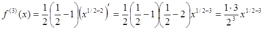
Пример 1: Найти третью производную от функции ![]() .
.
![]() ,
, ![]() ,
, ![]() .
.
Пример 2: Вычислить семнадцатую производную от функции ![]() в точке
в точке
![]() .
.
 ,
,
 ,
,
 ,
,
 …
…
Нетрудно заметить, что выражение для производной ![]() -го порядка может быть записано в виде
-го порядка может быть записано в виде 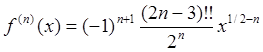 , откуда, подставляя
 ![]() , получаем
, получаем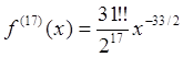 .
.
Наконец, положив ![]() , приходим к
, приходим к
окончательному результату 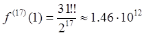 .
.
Определение 2: Дифференциалом ![]() — го порядка
— го порядка
называют величину
![]() .
.
(92)
Как правило, вместо ![]() пишут
пишут ![]() (не путать с
(не путать с ![]() ),
),
откуда непосредственно следует одна из форм записи для ![]() -й
-й
производной: ![]() .
.
Перейдем теперь к введению понятия ряда
Тейлора. Для начала сформулируем три задачи, с которыми мы в той или иной
степени уже встречались:
Задача 1: Вычислить с любой наперед заданной точностью (например 0.01) ![]() .
.
Отметим, что любой вычислительный алгоритм
базируется на четырех основных операциях (сложение, вычитание, умножение и
деление), которые могут быть реализованы, например, методом вычисления «в
столбик». Если при нахождении числа ![]() в качестве алгоритма
в качестве алгоритма
вычисления может быть предложен метод подбора: ![]()
(![]()
![]() и т.д.), то при нахождении
и т.д.), то при нахождении ![]() четкий алгоритм
четкий алгоритм
вычисления на первый взгляд отсутствует.
Задача 2: Аппроксимировать функцию ![]() на интервале
на интервале ![]() полиномом
полиномом ![]() с любой
с любой
наперед заданной точностью.
В предыдущем параграфе в качестве
наилучшей аппроксимации функции ![]() полиномом первой
полиномом первой
степени (линейной функцией) вблизи центра интервала ![]() была
была
предложена касательная ![]() , однако на границе
, однако на границе
интервала ![]() и данная аппроксимация абсолютно не
и данная аппроксимация абсолютно не
применима. По-видимому, аппроксимация полиномом более высокой степени ![]() , содержащим
, содержащим ![]() подгоночный
подгоночный
параметр, позволит улучшить точность приближения на всем интервале.
Задача 3: Найти предел функции ![]() .
.
Все три перечисленных задачи могут быть успешно
решены на основе формулы (ряда) Тейлора, отправной точкой для вывода которой
является задача 2.
Определение 3: Функциональным рядом называют ряд, элементами
(слагаемыми) которого являются функции  , где
, где ![]() является, вообще говоря, комплексной
является, вообще говоря, комплексной
переменной.
Определение 4: Степенным рядом называют функциональный ряд вида 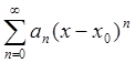 .
.
Предположим, что функция ![]() может
может
быть представлена в виде степенного ряда
![]() , тогда
, тогда
![]() ,
, ![]() ,
, ![]() ,
, ![]() , …
, … ![]() ,
,
откуда получаем  . (93)
О представлении функции в виде ряда (93) говорят как о
разложении в ряд Тейлора в окрестности точки ![]() .
.
Приведем несколько формул, задающих разложение в
ряд Тейлора основных элементарных функций в окрестности точки ![]() :
:
(94a)
(94b)
(94c)
(94d)
(94e)
Формулы (94a,b) нам уже знакомы (смотри (59), (72)).
Пример 3: Используя общую формулу (93) получить разложение (94b).
Поскольку все производные четного порядка в точке ![]() равны нулю (
равны нулю (![]() ), а
), а
значения нечетных производных вычисляются по формуле ![]() ,
,
имеем 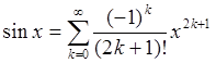 Ч.Т.Д.
Отметим, что, как и следовало ожидать, разложение нечетной
функции ![]() производится только по нечетным степеням
производится только по нечетным степеням
переменной ![]() . В разложение четной функции
. В разложение четной функции ![]() , наоборот, входят только четные степени
, наоборот, входят только четные степени
переменной ![]() .
.
На рис. 22 показана аппроксимация функции ![]() полиномами 1, 3, 5 и 7 степени, полученными
полиномами 1, 3, 5 и 7 степени, полученными
на основании формулы (94b).
Как видно из рисунка, повышение степени полинома влечет за собой увеличение
точности аппроксимации на всем интервале ![]() . При
. При
аппроксимации полиномом седьмой степени погрешность (максимальная на краях интервала)
не превосходит 10% (решение задачи 2).
В параграфе 13 было показано, что разложение (94b) позволяет без труда найти предел ![]() (решение задачи 3).
(решение задачи 3).
Пример 4: Используя общую формулу (93) получить разложение (94d).
Поскольку  , получаем
 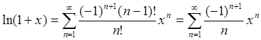 Ч.Т.Д.
Отметим, что в формулах (94d,e) натуральный логарифм и
степенная функция раскладываются в ряд Тейлора в окрестности аргумента, равного
единице (![]() ).
).
Разложение данных функций в окрестности нуля невозможно,
поскольку ![]() не определен в точке
не определен в точке ![]() , а для степенной функции
, а для степенной функции ![]() с показателем
с показателем ![]() при
при ![]() по крайней мере не определены все
по крайней мере не определены все
производные. С другой стороны, при аргументе ![]() , как
, как
функции, так и все их производные легко вычисляются.
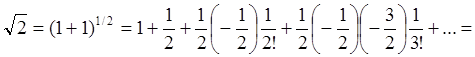
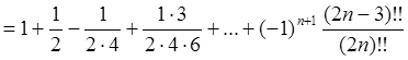
Пример 5: Используя формулы (94d,e), вычислить ![]() и
и ![]() с точностью 0.01.
с точностью 0.01.
Полагая ![]() ,
, ![]() , получаем:
, получаем:
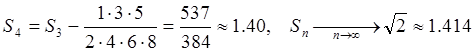
 (смотри (57)). Как было показано,
согласно теореме Лейбница, последовательность частичных сумм сходится:
![]()
![]() .
.
Перейдем к вычислению ![]() .
.
 (смотри (4)).
Сходимость ряда вновь следует из теоремы Лейбница:
знакочередующийся ряд, 
![]() , причем в данном случае последовательность
, причем в данном случае последовательность
частичных сумм сходится быстрее:

 (решение задачи 1).
Пример 6: Используя общую формулу (93), разложить полином ![]() в
в
ряд Тейлора в окрестности точек ![]() и
и ![]() .
.
Поскольку ![]() остальные
остальные ![]() , получаем:
, получаем:
при ![]() :
: ![]() , при
, при ![]() :
: ![]() .
.
Как и следовало ожидать, аппроксимация полинома третьей
степени полиномом той же самой (третьей) степени является точной (используя
формулу бинома Ньютона (27) легко показать, что обе аппроксимации совпадают при
всех ![]() ). В то же время, в окрестности точки
). В то же время, в окрестности точки ![]() (например, когда
(например, когда ![]() )
)
можно упростить исходную функцию, заменив ее с высокой точностью линейной ![]() (смотри рис. 23). В окрестности точки
(смотри рис. 23). В окрестности точки ![]() (например, когда
(например, когда ![]() )
)
исходная функция может быть аппроксимирована параболой ![]() .
.
Похожие материалы
- Определение степени с дробным показателем. Область определения неравенства
- Комбинированные уравнения. Указания для решения контрольных тестов
- Плоскости и их общие точки. Вычисление площади правильного треугольника
Информация о работе
Разложение в ряд Тейлора
Если функция f(x) имеет на некотором интервале, содержащем точку а, производные всех порядков, то к ней может быть применена формула Тейлора:
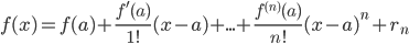 ,
,
где rn – так называемый остаточный член или остаток ряда, его можно оценить с помощью формулы Лагранжа:
 , где число x заключено между х и а.
- Решение онлайн
- Видеоинструкция
Если для некоторого значения х rn→0 при n→∞, то в пределе формула Тейлора превращается для этого значения в сходящийся ряд Тейлора:

Таким образом, функция f(x) может быть разложена в ряд Тейлора в рассматриваемой точке х, если:
- она имеет производные всех порядков;
- построенный ряд сходится в этой точке.
При а=0 получаем ряд, называемый рядом Маклорена:
Разложение простейших (элементарных) функций в ряд Маклорена:
Пример №1. Разложить в степенной ряд функцию f(x)=2x.
Решение. Найдем значения функции и ее производных при х=0
f(x) = 2x, f(0) = 20=1;
f'(x) = 2xln2, f'(0) = 20 ln2= ln2;
f»(x) = 2x ln22, f»(0) = 20 ln22= ln22;
…
f(n)(x) = 2x lnn2, f(n)(0) = 20 lnn2= lnn2.
Подставляя полученные значения производных в формулу ряда Тейлора, получим:

Радиус сходимости этого ряда равен бесконечности, поэтому данное разложение справедливо для -∞<x<+∞.
Пример №2. Написать ряд Тейлора по степеням (х+4) для функции f(x)=ex.
Решение. Находим производные функции ex и их значения в точке х=-4.
f(x) = еx, f(-4) = е-4;
f'(x) = еx, f'(-4) = е-4;
f»(x) = еx, f»(-4) = е-4;
…
f(n)(x) = еx, f(n)( -4) = е-4.
Следовательно, искомый ряд Тейлора функции имеет вид:
Данное разложение также справедливо для -∞<x<+∞.
Пример №3. Разложить функцию f(x)=lnx в ряд по степеням (х-1),
( т.е. в ряд Тейлора в окрестности точки х=1).
Решение. Находим производные данной функции.
f(x)=lnx, , , ,
f(1)=ln1=0, f'(1)=1, f»(1)=-1, f»'(1)=1*2,…, f(n)=(-1)n-1(n-1)!
Подставляя эти значения в формулу, получим искомый ряд Тейлора:
С помощью признака Даламбера можно убедиться, что ряд сходится при ½х-1½<1. Действительно,
Ряд сходится, если ½х-1½<1, т.е. при 0<x<2. При х=2 получаем знакочередующийся ряд, удовлетворяющий условиям признака Лейбница. При х=0 функция не определена. Таким образом, областью сходимости ряда Тейлора является полуоткрытый промежуток (0;2].
Пример №4. Разложить в степенной ряд функцию .
Решение. В разложении (1) заменяем х на -х2, получаем:
, -∞<x<∞
Пример №5. Разложить в ряд Маклорена функцию .
Решение. Имеем
Пользуясь формулой (4), можем записать:
подставляя вместо х в формулу –х, получим:
Отсюда находим: ln(1+x)-ln(1-x) = —
Раскрывая скобки, переставляя члены ряда и делая приведение подобных слагаемых, получим
. Этот ряд сходится в интервале (-1;1), так как он получен из двух рядов, каждый из которых сходится в этом интервале.
Замечание.
Формулами (1)-(5) можно пользоваться и для разложения соответствующих функций в ряд Тейлора, т.е. для разложения функций по целым положительным степеням (х-а). Для этого над заданной функцией необходимо произвести такие тождественные преобразования, чтобы получить одну из функций (1)-(5), в которой вместо х стоит k(х-а)m, где k – постоянное число, m – целое положительное число. Часто при этом удобно сделать замену переменной t=х-а и раскладывать полученную функцию относительно t в ряд Маклорена.
Этот метод основан на теореме о единственности разложения функции в степенной ряд. Сущность этой теоремы состоит в том, что в окрестности одной и той же точки не может быть получено два различных степенных ряда, которые бы сходились к одной и той же функции, каким бы способом ее разложение ни производилось.
Пример №5а. Разложить в ряд Маклорена функцию , указать область сходимости.
Решение. Сначала найдем 1-x-6x2=(1-3x)(1+2x), далее разложим дробь с помощью сервиса.
на элементарные:
Дробь 3/(1-3x) можно рассматривать как сумму бесконечно убывающей геометрической прогрессии знаменателем 3x, если |3x| < 1. Аналогично, дробь 2/(1+2x) как сумму бесконечно убывающей геометрической прогрессии знаменателем -2x, если |-2x| < 1. В результате получим разложение в степенной ряд
с областью сходимости |x| < 1/3.
Пример №6. Разложить функцию в ряд Тейлора в окрестности точки х=3.
Решение. Эту задачу можно решить, как и раньше, с помощью определения ряда Тейлора, для чего нужно найти производные функции и их значения при х=3. Однако проще будет воспользоваться имеющимся разложением (5):
=
Полученный ряд сходится при или –3<x-3<3, 0<x< 6 и является искомым рядом Тейлора для данной функции.
Пример №7. Написать ряд Тейлора по степеням (х-1) функции ln(x+2).
Решение.
Ряд сходится при , или -2 < x < 5.
Пример №8. Разложить функцию f(x)=sin(πx/4) в ряд Тейлора в окрестности точки x=2.
Решение. Сделаем замену t=х-2:
Воспользовавшись разложением (3), в котором на место х подставим π/4t, получим:
Полученный ряд сходится к заданной функции при -∞<π/4t<+∞, т.е. при (-∞<x<+∞).
Таким образом,
, (-∞<x<+∞)
Приближенные вычисления с помощью степенных рядов
Степенные ряды широко используются в приближенных вычислениях. С их помощью с заданной точностью можно вычислять значения корней, тригонометрических функций, логарифмов чисел, определенных интегралов. Ряды применяются также при интегрировании дифференциальных уравнений.
Рассмотрим разложение функции в степенной ряд:
Для того, чтобы вычислить приближенное значение функции в заданной точке х, принадлежащей области сходимости указанного ряда, в ее разложении оставляют первые n членов (n – конечное число), а остальные слагаемые отбрасывают:
Для оценки погрешности полученного приближенного значения необходимо оценить отброшенный остаток rn(x). Для этого применяют следующие приемы:
- если полученный ряд является знакочередующимся, то используется следующее свойство: для знакочередующегося ряда, удовлетворяющего условиям Лейбница, остаток ряда по абсолютной величине не превосходит первого отброшенного члена.
- если данный ряд знакопостоянный, то ряд, составленный из отброшенных членов, сравнивают с бесконечно убывающей геометрической прогрессией.
- в общем случае для оценки остатка ряда Тейлора можно воспользоваться формулой Лагранжа: a<c<x (или x<c<a).
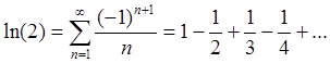
Пример №1. Вычислить ln(3) с точностью до 0,01.
Решение. Воспользуемся разложением , где x=1/2 (см. пример 5 в предыдущей теме):
Проверим, можем ли мы отбросить остаток после первых трех членов разложения, для этого оценим его с помощью суммы бесконечно убывающей геометрической прогрессии:
Таким образом, мы можем отбросить этот остаток и получаем
Пример №2. Вычислить с точностью до 0,0001.
Решение. Воспользуемся биномиальным рядом. Так как 53 является ближайшим к 130 кубом целого числа, то целесообразно число 130 представить в виде 130=53+5.
так как уже четвертый член полученного знакочередующегося ряда, удовлетворяющего признаку Лейбница, меньше требуемой точности:
, поэтому его и следующие за ним члены можно отбросить.
Многие практически нужные определенные или несобственные интегралы не могут быть вычислены с помощью формулы Ньютона-Лейбница, ибо ее применение связано с нахождением первообразной, часто не имеющей выражения в элементарных функциях. Бывает также, что нахождение первообразной возможно, но излишне трудоемко. Однако если подынтегральная функция раскладывается в степенной ряд, а пределы интегрирования принадлежат интервалу сходимости этого ряда, то возможно приближенное вычисление интеграла с наперед заданной точностью.
Пример №3. Вычислить интеграл ∫014sin(x)x с точностью до 10-5.
Решение. Соответствующий неопределенный интеграл не может быть выражен в элементарных функциях, т.е. представляет собой «неберущийся интеграл». Применить формулу Ньютона-Лейбница здесь нельзя. Вычислим интеграл приближенно.
Разделив почленно ряд для sinx на x , получим:
Интегрируя этот ряд почленно (это возможно, так как пределы интегрирования принадлежат интервалу сходимости данного ряда), получаем:
Так как полученный ряд удовлетворяет условиям Лейбница и достаточно взять сумму первых двух членов, чтобы получить искомое значение с заданной точностью.
Таким образом, находим
Пример №4. Вычислить интеграл ∫014ex2 с точностью до 0,001.
Решение.
![]()
Проверим, можем ли мы отбросить остаток после второго члена полученного ряда.
≈0.0001<0.001
Следовательно, .
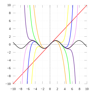
As the degree of the Taylor polynomial rises, it approaches the correct function. This image shows sin x and its Taylor approximations by polynomials of degree 1, 3, 5, 7, 9, 11, and 13 at x = 0.
In mathematics, the Taylor series or Taylor expansion of a function is an infinite sum of terms that are expressed in terms of the function’s derivatives at a single point. For most common functions, the function and the sum of its Taylor series are equal near this point. Taylor series are named after Brook Taylor, who introduced them in 1715. A Taylor series is also called a Maclaurin series when 0 is the point where the derivatives are considered, after Colin Maclaurin, who made extensive use of this special case of Taylor series in the mid-18th century.
The partial sum formed by the first n + 1 terms of a Taylor series is a polynomial of degree n that is called the nth Taylor polynomial of the function. Taylor polynomials are approximations of a function, which become generally better as n increases. Taylor’s theorem gives quantitative estimates on the error introduced by the use of such approximations. If the Taylor series of a function is convergent, its sum is the limit of the infinite sequence of the Taylor polynomials. A function may differ from the sum of its Taylor series, even if its Taylor series is convergent. A function is analytic at a point x if it is equal to the sum of its Taylor series in some open interval (or open disk in the complex plane) containing x. This implies that the function is analytic at every point of the interval (or disk).
Definition[edit]
The Taylor series of a real or complex-valued function f (x) that is infinitely differentiable at a real or complex number a is the power series

where n! denotes the factorial of n. In the more compact sigma notation, this can be written as

where f(n)(a) denotes the nth derivative of f evaluated at the point a. (The derivative of order zero of f is defined to be f itself and (x − a)0 and 0! are both defined to be 1.)
With a = 0, the Maclaurin series takes the form:[1]

or in the compact sigma notation:

Examples[edit]
The Taylor series of any polynomial is the polynomial itself.
The Maclaurin series of 1/1 − x is the geometric series

So, by substituting x for 1 − x, the Taylor series of 1/x at a = 1 is

By integrating the above Maclaurin series, we find the Maclaurin series of ln(1 − x), where ln denotes the natural logarithm:

The corresponding Taylor series of ln x at a = 1 is

and more generally, the corresponding Taylor series of ln x at an arbitrary nonzero point a is:

The Maclaurin series of the exponential function ex is

The above expansion holds because the derivative of ex with respect to x is also ex, and e0 equals 1. This leaves the terms (x − 0)n in the numerator and n! in the denominator of each term in the infinite sum.
History[edit]
The ancient Greek philosopher Zeno of Elea considered the problem of summing an infinite series to achieve a finite result, but rejected it as an impossibility;[2] the result was Zeno’s paradox. Later, Aristotle proposed a philosophical resolution of the paradox, but the mathematical content was apparently unresolved until taken up by Archimedes, as it had been prior to Aristotle by the Presocratic Atomist Democritus. It was through Archimedes’s method of exhaustion that an infinite number of progressive subdivisions could be performed to achieve a finite result.[3] Liu Hui independently employed a similar method a few centuries later.[4]
In the 14th century, the earliest examples of specific Taylor series (but not the general method) were given by Madhava of Sangamagrama.[5][6] Though no record of his work survives, writings of his followers in the Kerala school of astronomy and mathematics suggest that he found the Taylor series for the trigonometric functions of sine, cosine, and arctangent (see Madhava series). During the following two centuries his followers developed further series expansions and rational approximations.
In late 1670, James Gregory was shown in a letter from John Collins several Maclaurin series (

 and
and  ) derived by Isaac Newton, and told that Newton had developed a general method for expanding functions in series. Newton had in fact used a cumbersome method involving long division of series and term-by-term integration, but Gregory did not know it and set out to discover a general method for himself. In early 1671 Gregory discovered something like the general Maclaurin series and sent a letter to Collins including series for


 (the integral of
  ),
),  (the integral of sec, the inverse Gudermannian function),
  and
and  (the Gudermannian function). However, thinking that he had merely redeveloped a method by Newton, Gregory never described how he obtained these series, and it can only be inferred that he understood the general method by examining scratch work he had scribbled on the back of another letter from 1671.[7]
In 1691–1692, Isaac Newton wrote down an explicit statement of the Taylor and Maclaurin series in an unpublished version of his work De Quadratura Curvarum. However, this work was never completed and the relevant sections were omitted from the portions published in 1704 under the title Tractatus de Quadratura Curvarum.
It was not until 1715 that a general method for constructing these series for all functions for which they exist was finally published by Brook Taylor,[8] after whom the series are now named.
The Maclaurin series was named after Colin Maclaurin, a professor in Edinburgh, who published the special case of the Taylor result in the mid-18th century.
Analytic functions[edit]
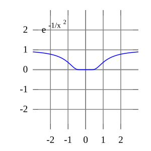
The function e(−1/x2) is not analytic at x = 0: the Taylor series is identically 0, although the function is not.
If f (x) is given by a convergent power series in an open disk centred at b in the complex plane (or an interval in the real line), it is said to be analytic in this region. Thus for x in this region, f is given by a convergent power series

Differentiating by x the above formula n times, then setting x = b gives:

and so the power series expansion agrees with the Taylor series. Thus a function is analytic in an open disk centered at b if and only if its Taylor series converges to the value of the function at each point of the disk.
If f (x) is equal to the sum of its Taylor series for all x in the complex plane, it is called entire. The polynomials, exponential function ex, and the trigonometric functions sine and cosine, are examples of entire functions. Examples of functions that are not entire include the square root, the logarithm, the trigonometric function tangent, and its inverse, arctan. For these functions the Taylor series do not converge if x is far from b. That is, the Taylor series diverges at x if the distance between x and b is larger than the radius of convergence. The Taylor series can be used to calculate the value of an entire function at every point, if the value of the function, and of all of its derivatives, are known at a single point.
Uses of the Taylor series for analytic functions include:
- The partial sums (the Taylor polynomials) of the series can be used as approximations of the function. These approximations are good if sufficiently many terms are included.
- Differentiation and integration of power series can be performed term by term and is hence particularly easy.
- An analytic function is uniquely extended to a holomorphic function on an open disk in the complex plane. This makes the machinery of complex analysis available.
- The (truncated) series can be used to compute function values numerically, (often by recasting the polynomial into the Chebyshev form and evaluating it with the Clenshaw algorithm).
- Algebraic operations can be done readily on the power series representation; for instance, Euler’s formula follows from Taylor series expansions for trigonometric and exponential functions. This result is of fundamental importance in such fields as harmonic analysis.
- Approximations using the first few terms of a Taylor series can make otherwise unsolvable problems possible for a restricted domain; this approach is often used in physics.
Approximation error and convergence[edit]
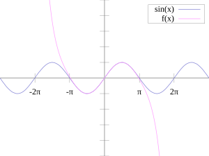
The sine function (blue) is closely approximated by its Taylor polynomial of degree 7 (pink) for a full period centered at the origin.

The Taylor polynomials for ln(1 + x) only provide accurate approximations in the range −1 < x ≤ 1. For x > 1, Taylor polynomials of higher degree provide worse approximations.

The Taylor approximations for ln(1 + x) (black). For x > 1, the approximations diverge.
Pictured is an accurate approximation of sin x around the point x = 0. The pink curve is a polynomial of degree seven:

The error in this approximation is no more than |x|9 / 9!. For a full cycle centered at the origin (−π < x < π) the error is less than 0.08215. In particular, for −1 < x < 1, the error is less than 0.000003.
In contrast, also shown is a picture of the natural logarithm function ln(1 + x) and some of its Taylor polynomials around a = 0. These approximations converge to the function only in the region −1 < x ≤ 1; outside of this region the higher-degree Taylor polynomials are worse approximations for the function.
The error incurred in approximating a function by its nth-degree Taylor polynomial is called the remainder or residual and is denoted by the function Rn(x). Taylor’s theorem can be used to obtain a bound on the size of the remainder.
In general, Taylor series need not be convergent at all. And in fact the set of functions with a convergent Taylor series is a meager set in the Fréchet space of smooth functions. And even if the Taylor series of a function f does converge, its limit need not in general be equal to the value of the function f (x). For example, the function
![{displaystyle f(x)={begin{cases}e^{-1/x^{2}}&{text{if }}xneq 0\[3mu]0&{text{if }}x=0end{cases}}}](https://wikimedia.org/api/rest_v1/media/math/render/svg/ae050e61cde6a0fdeda1f237f75846465579462d)
is infinitely differentiable at x = 0, and has all derivatives zero there. Consequently, the Taylor series of f (x) about x = 0 is identically zero. However, f (x) is not the zero function, so does not equal its Taylor series around the origin. Thus, f (x) is an example of a non-analytic smooth function.
In real analysis, this example shows that there are infinitely differentiable functions f (x) whose Taylor series are not equal to f (x) even if they converge. By contrast, the holomorphic functions studied in complex analysis always possess a convergent Taylor series, and even the Taylor series of meromorphic functions, which might have singularities, never converge to a value different from the function itself. The complex function e−1/z2, however, does not approach 0 when z approaches 0 along the imaginary axis, so it is not continuous in the complex plane and its Taylor series is undefined at 0.
More generally, every sequence of real or complex numbers can appear as coefficients in the Taylor series of an infinitely differentiable function defined on the real line, a consequence of Borel’s lemma. As a result, the radius of convergence of a Taylor series can be zero. There are even infinitely differentiable functions defined on the real line whose Taylor series have a radius of convergence 0 everywhere.[9]
A function cannot be written as a Taylor series centred at a singularity; in these cases, one can often still achieve a series expansion if one allows also negative powers of the variable x; see Laurent series. For example, f (x) = e−1/x2 can be written as a Laurent series.
Generalization[edit]
There is, however, a generalization[10][11] of the Taylor series that does converge to the value of the function itself for any bounded continuous function on (0,∞), using the calculus of finite differences. Specifically, one has the following theorem, due to Einar Hille, that for any t > 0,

Here Δn
h is the nth finite difference operator with step size h. The series is precisely the Taylor series, except that divided differences appear in place of differentiation: the series is formally similar to the Newton series. When the function f is analytic at a, the terms in the series converge to the terms of the Taylor series, and in this sense generalizes the usual Taylor series.
In general, for any infinite sequence ai, the following power series identity holds:

So in particular,

The series on the right is the expectation value of f (a + X), where X is a Poisson-distributed random variable that takes the value jh with probability e−t/h·(t/h)j/j!. Hence,

The law of large numbers implies that the identity holds.[12]
List of Maclaurin series of some common functions[edit]
Several important Maclaurin series expansions follow.[13] All these expansions are valid for complex arguments x.
Exponential function[edit]
The exponential function ex (in blue), and the sum of the first n + 1 terms of its Taylor series at 0 (in red).
The exponential function  (with base e) has Maclaurin series
 .
.

It converges for all x.
The exponential generating function of the Bell numbers is the exponential function of the predecessor of the exponential function:

Natural logarithm[edit]
The natural logarithm (with base e) has Maclaurin series

They converge for  . (In addition, the series for ln(1 − x) converges for x = −1, and the series for ln(1 + x) converges for x = 1.)
Geometric series[edit]
The geometric series and its derivatives have Maclaurin series

All are convergent for . These are special cases of the binomial series given in the next section.
Binomial series[edit]
The binomial series is the power series

whose coefficients are the generalized binomial coefficients

(If n = 0, this product is an empty product and has value 1.) It converges for for any real or complex number α.
When α = −1, this is essentially the infinite geometric series mentioned in the previous section. The special cases α = 1/2 and α = −1/2 give the square root function and its inverse:

When only the linear term is retained, this simplifies to the binomial approximation.
Trigonometric functions[edit]
The usual trigonometric functions and their inverses have the following Maclaurin series:
![{displaystyle {begin{aligned}sin x&=sum _{n=0}^{infty }{frac {(-1)^{n}}{(2n+1)!}}x^{2n+1}&&=x-{frac {x^{3}}{3!}}+{frac {x^{5}}{5!}}-cdots &&{text{for all }}x\[6pt]cos x&=sum _{n=0}^{infty }{frac {(-1)^{n}}{(2n)!}}x^{2n}&&=1-{frac {x^{2}}{2!}}+{frac {x^{4}}{4!}}-cdots &&{text{for all }}x\[6pt]tan x&=sum _{n=1}^{infty }{frac {B_{2n}(-4)^{n}left(1-4^{n}right)}{(2n)!}}x^{2n-1}&&=x+{frac {x^{3}}{3}}+{frac {2x^{5}}{15}}+cdots &&{text{for }}|x|<{frac {pi }{2}}\[6pt]sec x&=sum _{n=0}^{infty }{frac {(-1)^{n}E_{2n}}{(2n)!}}x^{2n}&&=1+{frac {x^{2}}{2}}+{frac {5x^{4}}{24}}+cdots &&{text{for }}|x|<{frac {pi }{2}}\[6pt]arcsin x&=sum _{n=0}^{infty }{frac {(2n)!}{4^{n}(n!)^{2}(2n+1)}}x^{2n+1}&&=x+{frac {x^{3}}{6}}+{frac {3x^{5}}{40}}+cdots &&{text{for }}|x|leq 1\[6pt]arccos x&={frac {pi }{2}}-arcsin x\&={frac {pi }{2}}-sum _{n=0}^{infty }{frac {(2n)!}{4^{n}(n!)^{2}(2n+1)}}x^{2n+1}&&={frac {pi }{2}}-x-{frac {x^{3}}{6}}-{frac {3x^{5}}{40}}-cdots &&{text{for }}|x|leq 1\[6pt]arctan x&=sum _{n=0}^{infty }{frac {(-1)^{n}}{2n+1}}x^{2n+1}&&=x-{frac {x^{3}}{3}}+{frac {x^{5}}{5}}-cdots &&{text{for }}|x|leq 1, xneq pm iend{aligned}}}](https://wikimedia.org/api/rest_v1/media/math/render/svg/158a0ae14d1c9e0d1dc21c268f7e2169b9066dc7)
All angles are expressed in radians. The numbers Bk appearing in the expansions of tan x are the Bernoulli numbers. The Ek in the expansion of sec x are Euler numbers.
Hyperbolic functions[edit]
The hyperbolic functions have Maclaurin series closely related to the series for the corresponding trigonometric functions:
![{displaystyle {begin{aligned}sinh x&=sum _{n=0}^{infty }{frac {x^{2n+1}}{(2n+1)!}}&&=x+{frac {x^{3}}{3!}}+{frac {x^{5}}{5!}}+cdots &&{text{for all }}x\[6pt]cosh x&=sum _{n=0}^{infty }{frac {x^{2n}}{(2n)!}}&&=1+{frac {x^{2}}{2!}}+{frac {x^{4}}{4!}}+cdots &&{text{for all }}x\[6pt]tanh x&=sum _{n=1}^{infty }{frac {B_{2n}4^{n}left(4^{n}-1right)}{(2n)!}}x^{2n-1}&&=x-{frac {x^{3}}{3}}+{frac {2x^{5}}{15}}-{frac {17x^{7}}{315}}+cdots &&{text{for }}|x|<{frac {pi }{2}}\[6pt]operatorname {arsinh} x&=sum _{n=0}^{infty }{frac {(-1)^{n}(2n)!}{4^{n}(n!)^{2}(2n+1)}}x^{2n+1}&&=x-{frac {x^{3}}{6}}+{frac {3x^{5}}{40}}-cdots &&{text{for }}|x|leq 1\[6pt]operatorname {artanh} x&=sum _{n=0}^{infty }{frac {x^{2n+1}}{2n+1}}&&=x+{frac {x^{3}}{3}}+{frac {x^{5}}{5}}+cdots &&{text{for }}|x|leq 1, xneq pm 1end{aligned}}}](https://wikimedia.org/api/rest_v1/media/math/render/svg/cda808c97562eca785bd172eb7739711b338730a)
The numbers Bk appearing in the series for tanh x are the Bernoulli numbers.
Polylogarithmic functions[edit]
The polylogarithms have these defining identities:


The Legendre chi functions are defined as follows:


And the formulas presented below are called inverse tangent integrals:


In statistical thermodynamics these formulas are of great importance.
Elliptic functions[edit]
The complete elliptic integrals of first kind K and of second kind E can be defined as follows:
![{displaystyle {frac {2}{pi }}K(x)=sum _{n=0}^{infty }{frac {[(2n)!]^{2}}{16^{n}(n!)^{4}}}x^{2n}}](https://wikimedia.org/api/rest_v1/media/math/render/svg/bc8e464983f3fdf2071ed149ed55bba842544a2d)
![{displaystyle {frac {2}{pi }}E(x)=sum _{n=0}^{infty }{frac {[(2n)!]^{2}}{(1-2n)16^{n}(n!)^{4}}}x^{2n}}](https://wikimedia.org/api/rest_v1/media/math/render/svg/85daf53e01f72f0f0c820811910a77974657052e)
The Jacobi theta functions describe the world of the elliptic modular functions and they have these Taylor series:


The regular partition number sequence P(n) has this generating function:
![{displaystyle vartheta _{00}(x)^{-1/6}vartheta _{01}(x)^{-2/3}{biggl [}{frac {vartheta _{00}(x)^{4}-vartheta _{01}(x)^{4}}{16,x}}{biggr ]}^{-1/24}=sum _{n=0}^{infty }P(n)x^{n}=prod _{k=1}^{infty }{frac {1}{1-x^{k}}}}](https://wikimedia.org/api/rest_v1/media/math/render/svg/3c898219336ceb853f972d83f60a14049d671523)
The strict partition number sequence Q(n) has that generating function:
![{displaystyle vartheta _{00}(x)^{1/6}vartheta _{01}(x)^{-1/3}{biggl [}{frac {vartheta _{00}(x)^{4}-vartheta _{01}(x)^{4}}{16,x}}{biggr ]}^{1/24}=sum _{n=0}^{infty }Q(n)x^{n}=prod _{k=1}^{infty }{frac {1}{1-x^{2k-1}}}}](https://wikimedia.org/api/rest_v1/media/math/render/svg/fa5dd403c225903926ad0c45788a5f1a0a5fb67c)
Calculation of Taylor series[edit]
Several methods exist for the calculation of Taylor series of a large number of functions. One can attempt to use the definition of the Taylor series, though this often requires generalizing the form of the coefficients according to a readily apparent pattern. Alternatively, one can use manipulations such as substitution, multiplication or division, addition or subtraction of standard Taylor series to construct the Taylor series of a function, by virtue of Taylor series being power series. In some cases, one can also derive the Taylor series by repeatedly applying integration by parts. Particularly convenient is the use of computer algebra systems to calculate Taylor series.
First example[edit]
In order to compute the 7th degree Maclaurin polynomial for the function
- ,

one may first rewrite the function as
- .

The Taylor series for the natural logarithm is (using the big O notation)

and for the cosine function
- .

The latter series expansion has a zero constant term, which enables us to substitute the second series into the first one and to easily omit terms of higher order than the 7th degree by using the big O notation:

Since the cosine is an even function, the coefficients for all the odd powers x, x3, x5, x7, … have to be zero.
Second example[edit]
Suppose we want the Taylor series at 0 of the function

We have for the exponential function

and, as in the first example,

Assume the power series is

Then multiplication with the denominator and substitution of the series of the cosine yields

Collecting the terms up to fourth order yields

The values of  can be found by comparison of coefficients with the top expression for , yielding:

Third example[edit]
Here we employ a method called «indirect expansion» to expand the given function. This method uses the known Taylor expansion of the exponential function. In order to expand (1 + x)ex as a Taylor series in x, we use the known Taylor series of function ex:

Thus,

Taylor series as definitions[edit]
Classically, algebraic functions are defined by an algebraic equation, and transcendental functions (including those discussed above) are defined by some property that holds for them, such as a differential equation. For example, the exponential function is the function which is equal to its own derivative everywhere, and assumes the value 1 at the origin. However, one may equally well define an analytic function by its Taylor series.
Taylor series are used to define functions and «operators» in diverse areas of mathematics. In particular, this is true in areas where the classical definitions of functions break down. For example, using Taylor series, one may extend analytic functions to sets of matrices and operators, such as the matrix exponential or matrix logarithm.
In other areas, such as formal analysis, it is more convenient to work directly with the power series themselves. Thus one may define a solution of a differential equation as a power series which, one hopes to prove, is the Taylor series of the desired solution.
Taylor series in several variables[edit]
The Taylor series may also be generalized to functions of more than one variable with[14][15]

For example, for a function  that depends on two variables, x and y, the Taylor series to second order about the point (a, b) is

where the subscripts denote the respective partial derivatives.
Second-order Taylor series in several variables[edit]
A second-order Taylor series expansion of a scalar-valued function of more than one variable can be written compactly as

where D f (a) is the gradient of f evaluated at x = a and D2 f (a) is the Hessian matrix. Applying the multi-index notation the Taylor series for several variables becomes

which is to be understood as a still more abbreviated multi-index version of the first equation of this paragraph, with a full analogy to the single variable case.
Example[edit]

Second-order Taylor series approximation (in orange) of a function f (x,y) = ex ln(1 + y) around the origin.
In order to compute a second-order Taylor series expansion around point (a, b) = (0, 0) of the function

one first computes all the necessary partial derivatives:
![{displaystyle {begin{aligned}f_{x}&=e^{x}ln(1+y)\[6pt]f_{y}&={frac {e^{x}}{1+y}}\[6pt]f_{xx}&=e^{x}ln(1+y)\[6pt]f_{yy}&=-{frac {e^{x}}{(1+y)^{2}}}\[6pt]f_{xy}&=f_{yx}={frac {e^{x}}{1+y}}.end{aligned}}}](https://wikimedia.org/api/rest_v1/media/math/render/svg/80a9f65e179df2db5256dc15097892be2ded7c6d)
Evaluating these derivatives at the origin gives the Taylor coefficients

Substituting these values in to the general formula

produces

Since ln(1 + y) is analytic in |y| < 1, we have

Comparison with Fourier series[edit]
The trigonometric Fourier series enables one to express a periodic function (or a function defined on a closed interval [a,b]) as an infinite sum of trigonometric functions (sines and cosines). In this sense, the Fourier series is analogous to Taylor series, since the latter allows one to express a function as an infinite sum of powers. Nevertheless, the two series differ from each other in several relevant issues:
- The finite truncations of the Taylor series of f (x) about the point x = a are all exactly equal to f at a. In contrast, the Fourier series is computed by integrating over an entire interval, so there is generally no such point where all the finite truncations of the series are exact.
- The computation of Taylor series requires the knowledge of the function on an arbitrary small neighbourhood of a point, whereas the computation of the Fourier series requires knowing the function on its whole domain interval. In a certain sense one could say that the Taylor series is «local» and the Fourier series is «global».
- The Taylor series is defined for a function which has infinitely many derivatives at a single point, whereas the Fourier series is defined for any integrable function. In particular, the function could be nowhere differentiable. (For example, f (x) could be a Weierstrass function.)
- The convergence of both series has very different properties. Even if the Taylor series has positive convergence radius, the resulting series may not coincide with the function; but if the function is analytic then the series converges pointwise to the function, and uniformly on every compact subset of the convergence interval. Concerning the Fourier series, if the function is square-integrable then the series converges in quadratic mean, but additional requirements are needed to ensure the pointwise or uniform convergence (for instance, if the function is periodic and of class C1 then the convergence is uniform).
- Finally, in practice one wants to approximate the function with a finite number of terms, say with a Taylor polynomial or a partial sum of the trigonometric series, respectively. In the case of the Taylor series the error is very small in a neighbourhood of the point where it is computed, while it may be very large at a distant point. In the case of the Fourier series the error is distributed along the domain of the function.
See also[edit]
- Asymptotic expansion
- Generating function
- Laurent series
- Madhava series
- Newton’s divided difference interpolation
- Padé approximant
- Puiseux series
- Shift operator
Notes[edit]
- ^ Thomas & Finney 1996, §8.9
- ^ Lindberg, David (2007). The Beginnings of Western Science (2nd ed.). University of Chicago Press. p. 33. ISBN 978-0-226-48205-7.
- ^ Kline, M. (1990). Mathematical Thought from Ancient to Modern Times. New York: Oxford University Press. pp. 35–37. ISBN 0-19-506135-7.
- ^ Boyer, C.; Merzbach, U. (1991). A History of Mathematics (Second revised ed.). John Wiley and Sons. pp. 202–203. ISBN 0-471-09763-2.
- ^ «Neither Newton nor Leibniz – The Pre-History of Calculus and Celestial Mechanics in Medieval Kerala» (PDF). MAT 314. Canisius College. Archived (PDF) from the original on 2015-02-23. Retrieved 2006-07-09.
- ^ S. G. Dani (2012). «Ancient Indian Mathematics – A Conspectus». Resonance. 17 (3): 236–246. doi:10.1007/s12045-012-0022-y. S2CID 120553186.
- ^ Turnbull, Herbert Westren, ed. (1939). James Gregory; Tercentenary Memorial Volume. G. Bell & Sons. pp. 168–174.Roy, Ranjan (1990). «The Discovery of the Series Formula for π by Leibniz, Gregory and Nilakantha» (PDF). Mathematics Magazine. 63 (5): 291–306. doi:10.1080/0025570X.1990.11977541.Malet, Antoni (1993). «James Gregorie on Tangents and the «Taylor» Rule for Series Expansions». Archive for History of Exact Sciences. 46 (2): 97–137. doi:10.1007/BF00375656. JSTOR 41133959.
- ^ Taylor, Brook (1715). Methodus Incrementorum Directa et Inversa [Direct and Reverse Methods of Incrementation] (in Latin). London. p. 21–23 (Prop. VII, Thm. 3, Cor. 2). Translated into English in Struik, D. J. (1969). A Source Book in Mathematics 1200–1800. Harvard University Press. pp. 329–332. ISBN 978-0-674-82355-6. Re-translated into English by Ian Bruce (2007) as Methodus Incrementorum Directa & Inversa, 17centurymaths.com.Feigenbaum, L. (1985). «Brook Taylor and the method of increments». Archive for History of Exact Sciences. 34 (1–2): 1–140. doi:10.1007/bf00329903.
- ^ Rudin, Walter (1980), Real and Complex Analysis, New Delhi: McGraw-Hill, p. 418, Exercise 13, ISBN 0-07-099557-5
- ^ Feller, William (2003) [1971]. An introduction to probability theory and its applications. Vol. 2 (3rd ed.). Wiley. pp. 230–2. ISBN 9789971512989. OCLC 818811840.
- ^ Hille, Einar; Phillips, Ralph S. (1957), Functional analysis and semi-groups, AMS Colloquium Publications, vol. 31, American Mathematical Society, pp. 300–327.
- ^ Feller 2003, p. 231
- ^ Most of these can be found in (Abramowitz & Stegun 1970).
- ^ Hörmander, Lars (2002) [1990]. «1. Test Functions §1.1. A review of Differential Calculus». The analysis of partial differential operators. Vol. 1 (2nd ed.). Springer. Eqq. 1.1.7 and 1.1.7′. doi:10.1007/978-3-642-61497-2_2. ISBN 978-3-642-61497-2.
- ^ Kolk, Johan A.C.; Duistermaat, J.J. (2010). «Taylor Expansion in Several Variables». Distributions: Theory and applications. Birkhauser. pp. 59–63. doi:10.1007/978-0-8176-4675-2_6. ISBN 978-0-8176-4672-1.
References[edit]
- Abramowitz, Milton; Stegun, Irene A. (1970), Handbook of Mathematical Functions with Formulas, Graphs, and Mathematical Tables, New York: Dover Publications, Ninth printing
- Thomas, George B. Jr.; Finney, Ross L. (1996), Calculus and Analytic Geometry (9th ed.), Addison Wesley, ISBN 0-201-53174-7
- Greenberg, Michael (1998), Advanced Engineering Mathematics (2nd ed.), Prentice Hall, ISBN 0-13-321431-1
- Roy, Ranjan (2021) [1st ed. 2011]. Series and Products in the Development of Mathematics. Vol. 1 (2nd ed.). Cambridge University Press.
External links[edit]
- «Taylor series», Encyclopedia of Mathematics, EMS Press, 2001 [1994]
- Weisstein, Eric W. «Taylor Series». MathWorld.