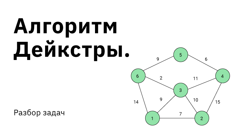
Алгоритм Дейкстры. Разбор Задач
Время на прочтение
7 мин
Количество просмотров 36K
Поиск оптимального пути в графе. Такая задача встречается довольно часто и в повседневной жизни, и в мире технологий. Справиться с такими вызовами помогает подход, который должен быть в арсенале каждого программиста — алгоритм Дейкстры.
Если вы хотите найти ответить на вопросы, чем этот алгоритм лучше BFS (поиска в ширину), при каких условиях алгоритм применим, и какие теоретические и практические задачи можно с его помощью решать, читайте далее.
Введение
Алгоритм Дейкстры работает на ориентированных (с некоторыми дополнениями и на неориентированных) графах, и призван искать кратчайшие пути между заданной вершиной и всеми остальными вершинами в графе.
Как правило, граф обозначают как набор вершин и рёбер  где число рёбер может быть задано
  , а вершин числом
Для каждого ребра в графе задан неотрицательный вес  , а также вершина, из которой осуществляется поиск оптимальных путей.
Алгоритм Дейкстры может найти кратчайший путь между вершинами  и
и  в графе, только если существует хотя бы один путь между этими вершинами. Если это условие не выполняется, то алгоритм отработает корректно, вернув значение «бесконечность» для пары несвязанных вершин.
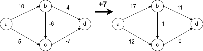
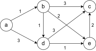
Условие неотрицательности весов рёбер крайне важно и от него нельзя просто избавиться. Не получится свести задачу к решаемой алгоритмом Дейкстры, прибавив наибольший по модулю вес ко всем рёбрам. Это может изменить оптимальный маршрут. На рисунке видно, что в первом случае оптимальный путь между  и
и  (сумма рёбер на пути наименьшая) изменяется при такой манипуляции. В оригинале путь проходит через
  , а после добавления семёрки ко всем рёбрам, оптимальный путь проходит через
Как ведёт себя алгоритм Дейкстры на исходном графе, мы разберём, когда выпишем алгоритм. Но для начала зададимся другим вопросом: «почему не применить поиск в ширину для нашего графа?». Известно, что метод BFS находит оптимальный путь от произвольной вершины в ориентированном графе до любой другой вершины, но это справедливо только для рёбер с единичным весом.
Свести задачу к решаемой BFS можно, но если заменить все рёбра неединичной длины  рёбрами длины
  , то граф очень разрастётся, и это приведёт к огромному числу действий при вычислении оптимального маршрута.
Чтобы этого избежать предлагается использовать алгоритм Дейкстры. Опишем его:
Инициализация:
Основный цикл алгоритма:
- Пока все вершины не исследованы (или формально
 ), повторяем:
 ), повторяем:
В итоге исполнения этого алгоритма, массив  будет содержать все оптимальные пути, исходящие из .
Примеры работы
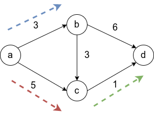
Рассмотрим граф выше, в нём будем искать пути от до всего остального.
Первый шаг алгоритма определит, что кратчайший путь до  проходит по направлению синей стрелки и зафиксирует кратчайший путь. Второй шаг рассмотрит, все возможные варианты
 ![inline A[v] + l_{vw}](https://habrastorage.org/getpro/habr/post_images/c10/6ca/2df/c106ca2df0651dd2d791b59d6959e8fb.svg) и окажется, что оптимальный вариант двигаться вдоль красной стрелки, поскольку
и окажется, что оптимальный вариант двигаться вдоль красной стрелки, поскольку  меньше, чем
  и
и  Добавляется длина кратчайшего пути до
  . И наконец, третьим шагом, когда три вершины
  уже лежат в
  , остается рассмотреть только два ребра и выбрать, лежащее вдоль зеленой стрелки.
Теперь рассмотрим граф с отрицательными весами, упомянутый выше. Напомню, алгоритм Дейкстры на таком графе может работать некорректно.
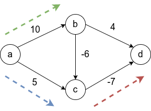
Первым шагом отбирается ребро вдоль синей стрелки, поскольку это ребро наименьшего веса из исходной вершины. Затем выбирается ребро  Это зафиксирует навсегда неверный путь от к , в то время как оптимальный путь проходит через центр с отрицательным весом. Последним шагом, будет добавлена вершина .
Оценка сложности алгоритма
К этому моменту мы разобрали сам алгоритм, ограничения, накладываемые на его работу и ряд примеров его применения. Давайте упомянем какова вычислительная сложность этого алгоритма, поскольку это пригодится нам для решения задач, ради которых затевалась эта статья.
Базовый подход, основанный на циклах, предполагает проход по всем рёбрам каждого узла, что приводит к сложности  .
.
Эффективная реализация предполагает использование кучи. Об этой структуре данных можно сказать коротко: она позволяет выполнять две операции за логарифмическое время. Первая операция — получение узла в дереве, с наименьшим ключом, и, вторая операция, вставка нового узла в дерево с новым ключом.
Что еще можно сказать о куче:
- это сбалансированное бинарное дерево,
- ключ текущего узла всегда меньше, либо равен ключей дочерних узлов.
Интересную задачу с использованием куч я разбирал ранее в этом посте.
Используя кучу в алгоритме Дейкстры, где в качестве ключей используются расстояния от вершины в неисследованной части графа (в алгоритме это  ), до ближайшей вершины в уже покрытом (это множество вершин ), можно сократить вычислительную сложность до
  Доказательство справедливости этих оценок я оставляю за пределами этой статьи.
Далее перейдём к разбору задач!
Задача №1
Будем называть узким местом пути в графе ребро максимальной длины в этом пути. Путём с минимальным узким местом назовём такой путь между вершинами и , что не существует другого пути  , чьё узкое место меньше по длине. Требуется построить алгоритм, который вычисляет путь с минимальным узким местом для двух данных вершин в графе. Асимптотическая сложность такого алгоритма должна быть
Решение
По условию задачи ребро с большим весом трактуется как узкое место. Вес в этом случае можно воспринимать как цену за проход по ребру. В результате решения задачи хотелось бы получить алгоритм, способный строить маршруты между узлами так, чтобы, если мы захотим провести любой другой путь, он будет содержать более тяжелые рёбра.
В случае классической задачи, поиска пути минимальной длины между двумя вершинами графа, мы поддерживаем в каждой посещенной алгоритмом вершине графа минимальную длину пути до этой вершины. Здесь стоит оговориться, что будем именовать множество посещенными вершинами, а часть графа, для которой еще нужно найти величину пути или узкого места.
В отличии от классического алгоритма, решение этой задачи должно поддерживать величину актуального узкого места пути, приводящего в вершину  . А при добавлении новой вершины из , мы должны смотреть не увеличивает ли ребро
  величину узкого места пути, которое теперь приводит в
  .
.
Если ребро увеличивает узкое место, то лучше рассмотреть вершину  , ребро
  до которой легче . Поиск неувеличивающих узкое место ребёр нужно осуществлять не только среди соседей определенного узла
  , но и среди всех , поскольку отдавая предпочтение вершине, путь в которую имеет наименьшее узкое место в данный момент, мы гарантируем, что мы не ухудшаем ситуацию для других вершин.
Последнее можно проиллюстрировать примером: если путь, оканчивающийся в вершине  имеет узкое место величины
  , и есть вершина
  с ребром
  веса
веса  , и
, и  с ребром
  веса , то предпочтение отдаётся , алгоритм даст верный результат в обоих случая, если существует
  веса или веса
  .
.
В результате разбора выше, предлагается руководствоваться следующей формулой при выборе очередной вершины из непосещенных и обновлении величин, которые мы поддерживаем.
![A(u) = min_{v in X}left(max left[A(v), wleft(v,uright)right]right), , u in V - X](https://habrastorage.org/getpro/habr/post_images/6bf/459/cbd/6bf459cbdc59a4ffaf8b7bfe68ed0f27.svg)
Стоит пояснить, что поиск по осуществляется, только для существующих связей  а
а  это вес ребра
  .
.
Задача №2
Предлагается решить более практическую задачу. Пусть городов, между ними существуют пути, заданные массивом edges[i] = [city_a, city_b, distance_ab], а также дано целое число mileage.
Требуется найти такой город из данных, из которого можно добраться до наименьшего числа городов не превысив mileage.
Стоит отметить, что граф неориентированый, т.е. по пути между городами можно двигаться в обе стороны, а длина пути между городами a и c может быть получена как сумма длин путей a -> b и b -> c, если есть маршрут a -> b -> c
Решение
С решением данной проблемы нам поможет алгоритм Дейкстры и описанная выше реализация с помощью кучи. Поставщиком этой структуры данных станет библиотека heapq в Python.
Будем использовать алгоритм Дейкстры для того, чтобы подсчитать количество соседних городов, расстояние до которых меньше mileage, для каждого из городов. Соберем количества соседей в в одном месте и найдем минимум из них.
Поскольку наш граф неориентированный, то из любой его вершины можно добраться до произвольной вершины . Будем использовать алгоритм Дейкстры для того, чтобы для каждого из городов в графе построить кратчайшие пути до всех остальных городов, мы это уже умеем делать в теории. И чтобы, оптимизировать этот процесс, будем в его течении сразу отвергать пути, которые превышают mileage, а не делать постфактум, когда все пути получены.
Давайте опишем функцию решения:
def least_reachable_city(n, edges, mileage):
        """
        входные параметры:
            n --- количество городов,
            edges --- тройки (a, b, distance_ab),
            mileage --- максимально допустимое расстояние между городами
            для соседства
        """
        # заполняем список смежности (adjacency list), в нашем случае это
        # словарь, в котором ключи это города, а значения --- пары
        # (<другой_город>, <расстояние_до_него>)

        graph = {}
        for u, v, w in edges:
            if graph.get(u, None) is None:
                graph[u] = [(v, w)]
            else:
                graph[u].append((v, w))
            if graph.get(v, None) is None:
                graph[v] = [(u, w)]
            else:
                graph[v].append((u, w))

        # локально объявим функцию, которая будет считать кратчайшие пути в
        # графе от вершины, до всех вершин, удовлетворяющих условию
        def num_reachable_neighbors(city):
            # создаем кучу, из одного элемента с парой, задающей нулевую
            # длину пути до самого исходного города
            heap = [(0, city)]
            # и массив, содержащий города и кратчайшие
            # расстояния до них от исходного
            distances = {}
            # затем, пока куча не пуста, извлекаем ближайший
            # от посещенных городов город
            while heap:
                currDist, neighb = heapq.heappop(heap)
                # если кратчайшее ребро ведет к городу, где мы уже знаем
                # оптимальный маршрут, то завершаем итерацию
                if neighb in distances:
                    continue
                # в остальных случаях, и если сосед не является отправным
                # городом, мы добавляем новую запись в массив кратчайших расстояний
                if neighb != city:
                    distances[neighb] = currDist
                # обрабатываем всех смежных городов с соседом, добавляя их в кучу
                # но только если: а) до них еще не известен кратчайший маршрут и б) путь до них через neighb не выходит за пределы mileage
                for node, d in graph[neighb]:
                    if node in distances:
                        continue
                    if currDist + d <= mileage:
                        heapq.heappush(heap, (currDist + d, node))
            # возвращаем количество городов, прошедших проверку
            return len(distances)

        # выполним поиск соседей для каждого из городов
        cities_neighbors = {num_reachable_neighbors(city): city for city in range(n)}
        # вернём номер города, у которого наименьшее число соседей
        # в пределах досигаемости
        return cities_neighbors[min(cities_neighbors)]
В функции выше, в комментариях, подробно описывается, как метод Дейкстры, реализованный на куче позволяет найти расстояния до всех городов, в пределах `mileage`. Основную сложность для понимания предстваляет цикл, работающий с кучей.
Заключение
Алгоритм Дейкстры это мощный инструмент в мире работы с графами, область применения его крайне широка. С его помощью можно оценить даже целесообразность добавления новой ветки метро, новой дороги или маршрута в компьютерной сети. Он прост в исполнении и интуитивно понятен, как другие жадные (greedy) алгоритмы. Вычислительная сложность решений задач с его помощью зачастую не выше  . При некоторых условиях может достигать линейной сложности (существует алгоритм линейной сложности, решающий первую задачу, при условии, что граф неориентированный).
Стоит еще раз отметить, что алгоритм не работает, когда в графе существуют отрицательные веса. Для этого существует подход динамического программирования — алгоритм Беллмана – Форда, что может послужить темой другой статьи. Несмотря на это, алгоритм Дейкстры является представителем идеального баланса простоты и мощи, для решения прикладных задач.
Статья подготовлена в преддверии старта курса «Алгоритмы для разработчиков». Узнать о курсе подробнее, а также зарегистрироваться на бесплатный демоурок можно по ссылке.
Информация
[1] Условия задач взяты из книги «Algorithms Illuminated: Part 2: Graph Algorithms and Data Structures» от Tim Roughgarden,
[2] и с сайта leetcode.com.
[3] Решения авторские.
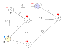
Рассмотрим пример нахождение кратчайшего пути. Дана сеть автомобильных дорог, соединяющих области города. Некоторые дороги односторонние. Найти кратчайшие пути от центра города до каждого города области.
Для решения указанной задачи можно использовать алгоритм Дейкстры — алгоритм на графах, изобретённый нидерландским ученым Э. Дейкстрой в 1959 году. Находит кратчайшее расстояние от одной из вершин графа до всех остальных. Работает только для графов без рёбер отрицательного веса.
Пусть требуется найти кратчайшие расстояния от 1-й вершины до всех остальных.
Кружками обозначены вершины, линиями – пути между ними (ребра графа). В кружках обозначены номера вершин, над ребрами обозначен их вес – длина пути. Рядом с каждой вершиной красным обозначена метка – длина кратчайшего пути в эту вершину из вершины 1.

Инициализация
Метка самой вершины 1 полагается равной 0, метки остальных вершин – недостижимо большое число (в идеале — бесконечность). Это отражает то, что расстояния от вершины 1 до других вершин пока неизвестны. Все вершины графа помечаются как непосещенные.

Первый шаг
Минимальную метку имеет вершина 1. Её соседями являются вершины 2, 3 и 6. Обходим соседей вершины по очереди.
Первый сосед вершины 1 – вершина 2, потому что длина пути до неё минимальна. Длина пути в неё через вершину 1 равна сумме кратчайшего расстояния до вершины 1 (значению её метки) и длины ребра, идущего из 1-й во 2-ю, то есть 0 + 7 = 7. Это меньше текущей метки вершины 2 (10000), поэтому новая метка 2-й вершины равна 7.

Аналогично находим длины пути для всех других соседей (вершины 3 и 6).
Все соседи вершины 1 проверены. Текущее минимальное расстояние до вершины 1 считается окончательным и пересмотру не подлежит. Вершина 1 отмечается как посещенная.
Второй шаг
Шаг 1 алгоритма повторяется. Снова находим «ближайшую» из непосещенных вершин. Это вершина 2 с меткой 7.
Снова пытаемся уменьшить метки соседей выбранной вершины, пытаясь пройти в них через 2-ю вершину. Соседями вершины 2 являются вершины 1, 3 и 4.
Вершина 1 уже посещена. Следующий сосед вершины 2 — вершина 3, так как имеет минимальную метку из вершин, отмеченных как не посещённые. Если идти в неё через 2, то длина такого пути будет равна 17 (7 + 10 = 17). Но текущая метка третьей вершины равна 9, а 9 < 17, поэтому метка не меняется.

Ещё один сосед вершины 2 — вершина 4. Если идти в неё через 2-ю, то длина такого пути будет равна 22 (7 + 15 = 22). Поскольку 22<10000, устанавливаем метку вершины 4 равной 22.
Все соседи вершины 2 просмотрены, помечаем её как посещенную.
Третий шаг
Повторяем шаг алгоритма, выбрав вершину 3. После её «обработки» получим следующие результаты.

Четвертый шаг

Пятый шаг

Шестой шаг

Таким образом, кратчайшим путем из вершины 1 в вершину 5 будет путь через вершины 1 — 3 — 6 — 5, поскольку таким путем мы набираем минимальный вес, равный 20.
Займемся выводом кратчайшего пути. Мы знаем длину пути для каждой вершины, и теперь будем рассматривать вершины с конца. Рассматриваем конечную вершину (в данном случае — вершина 5), и для всех вершин, с которой она связана, находим длину пути, вычитая вес соответствующего ребра из длины пути конечной вершины.
Так, вершина 5 имеет длину пути 20. Она связана с вершинами 6 и 4.
Для вершины 6 получим вес 20 — 9 = 11 (совпал).
Для вершины 4 получим вес 20 — 6 = 14 (не совпал).
Если в результате мы получим значение, которое совпадает с длиной пути рассматриваемой вершины (в данном случае — вершина 6), то именно из нее был осуществлен переход в конечную вершину. Отмечаем эту вершину на искомом пути.
Далее определяем ребро, через которое мы попали в вершину 6. И так пока не дойдем до начала.
Если в результате такого обхода у нас на каком-то шаге совпадут значения для нескольких вершин, то можно взять любую из них — несколько путей будут иметь одинаковую длину.
Реализация алгоритма Дейкстры
Для хранения весов графа используется квадратная матрица. В заголовках строк и столбцов находятся вершины графа. А веса дуг графа размещаются во внутренних ячейках таблицы. Граф не содержит петель, поэтому на главной диагонали матрицы содержатся нулевые значения.
| 1 | 2 | 3 | 4 | 5 | 6 | |
| 1 | 0 | 7 | 9 | 0 | 0 | 14 |
| 2 | 7 | 0 | 10 | 15 | 0 | 0 |
| 3 | 9 | 10 | 0 | 11 | 0 | 2 |
| 4 | 0 | 15 | 11 | 0 | 6 | 0 |
| 5 | 0 | 0 | 0 | 6 | 0 | 9 |
| 6 | 14 | 0 | 2 | 0 | 9 | 0 |
Реализация на C++
1
2
3
4
5
6
7
8
9
10
11
12
13
14
15
16
17
18
19
20
21
22
23
24
25
26
27
28
29
30
31
32
33
34
35
36
37
38
39
40
41
42
43
44
45
46
47
48
49
50
51
52
53
54
55
56
57
58
59
60
61
62
63
64
65
66
67
68
69
70
71
72
73
74
75
76
77
78
79
80
81
82
83
84
85
86
87
88
89
90
91
92
93
94
95
96
97
98
99
100
101
102
103
#define _CRT_SECURE_NO_WARNINGS
#include <stdio.h>
#include <stdlib.h>
#define SIZE 6
int main()
{
int a[SIZE][SIZE]; // матрица связей
int d[SIZE]; // минимальное расстояние
int v[SIZE]; // посещенные вершины
int temp, minindex, min;
int begin_index = 0;
system(«chcp 1251»);
system(«cls»);
// Инициализация матрицы связей
for (int i = 0; i<SIZE; i++)
{
a[i][i] = 0;
for (int j = i + 1; j<SIZE; j++) {
printf(«Введите расстояние %d — %d: «, i + 1, j + 1);
scanf(«%d», &temp);
a[i][j] = temp;
a[j][i] = temp;
}
}
// Вывод матрицы связей
for (int i = 0; i<SIZE; i++)
{
for (int j = 0; j<SIZE; j++)
printf(«%5d «, a[i][j]);
printf(«n»);
}
//Инициализация вершин и расстояний
for (int i = 0; i<SIZE; i++)
{
d[i] = 10000;
v[i] = 1;
}
d[begin_index] = 0;
// Шаг алгоритма
do {
minindex = 10000;
min = 10000;
for (int i = 0; i<SIZE; i++)
{ // Если вершину ещё не обошли и вес меньше min
if ((v[i] == 1) && (d[i]<min))
{ // Переприсваиваем значения
min = d[i];
minindex = i;
}
}
// Добавляем найденный минимальный вес
// к текущему весу вершины
// и сравниваем с текущим минимальным весом вершины
if (minindex != 10000)
{
for (int i = 0; i<SIZE; i++)
{
if (a[minindex][i] > 0)
{
temp = min + a[minindex][i];
if (temp < d[i])
{
d[i] = temp;
}
}
}
v[minindex] = 0;
}
} while (minindex < 10000);
// Вывод кратчайших расстояний до вершин
printf(«nКратчайшие расстояния до вершин: n»);
for (int i = 0; i<SIZE; i++)
printf(«%5d «, d[i]);
// Восстановление пути
int ver[SIZE]; // массив посещенных вершин
int end = 4; // индекс конечной вершины = 5 — 1
ver[0] = end + 1; // начальный элемент — конечная вершина
int k = 1; // индекс предыдущей вершины
int weight = d[end]; // вес конечной вершины
while (end != begin_index) // пока не дошли до начальной вершины
{
for (int i = 0; i<SIZE; i++) // просматриваем все вершины
if (a[i][end] != 0) // если связь есть
{
int temp = weight — a[i][end]; // определяем вес пути из предыдущей вершины
if (temp == d[i]) // если вес совпал с рассчитанным
{ // значит из этой вершины и был переход
weight = temp; // сохраняем новый вес
end = i; // сохраняем предыдущую вершину
ver[k] = i + 1; // и записываем ее в массив
k++;
}
}
}
// Вывод пути (начальная вершина оказалась в конце массива из k элементов)
printf(«nВывод кратчайшего путиn»);
for (int i = k — 1; i >= 0; i—)
printf(«%3d «, ver[i]);
getchar(); getchar();
return 0;
}
Результат выполнения

Назад: Алгоритмизация
Алгоритм Дейкстры (англ. Dijkstra’s algorithm) находит кратчайшие пути от заданной вершины $s$ до всех остальных в графе без ребер отрицательного веса.
Существует два основных варианта алгоритма, время работы которых составляет $O(n^2)$ и $O(m log n)$, где $n$ — число вершин, а $m$ — число ребер.
#Основная идея
Заведём массив $d$, в котором для каждой вершины $v$ будем хранить текущую длину $d_v$ кратчайшего пути из $s$ в $v$. Изначально $d_s = 0$, а для всех остальных вершин расстояние равно бесконечности (или любому числу, которое заведомо больше максимально возможного расстояния).
Во время работы алгоритма мы будем постепенно обновлять этот массив, находя более оптимальные пути к вершинам и уменьшая расстояние до них. Когда мы узнаем, что найденный путь до какой-то вершины $v$ оптимальный, мы будем помечать эту вершину, поставив единицу ($a_v=1$) в специальном массиве $a$, изначально заполненном нулями.
Сам алгоритм состоит из $n$ итераций, на каждой из которых выбирается вершина $v$ с наименьшей величиной $d_v$ среди ещё не помеченных:
$$
v = argmin_{u | a_u=0} d_u
$$
(Заметим, что на первой итерации выбрана будет стартовая вершина $s$.)
Выбранная вершина отмечается в массиве $a$, после чего из из вершины $v$ производятся релаксации: просматриваем все исходящие рёбра $(v,u)$ и для каждой такой вершины $u$ пытаемся улучшить значение $d_u$, выполнив присвоение
$$
d_u = min (d_u, d_v + w)
$$
где $w$ — длина ребра $(v, u)$.
На этом текущая итерация заканчивается, и алгоритм переходит к следующей: снова выбирается вершина с наименьшей величиной $d$, из неё производятся релаксации, и так далее. После $n$ итераций, все вершины графа станут помеченными, и алгоритм завершает свою работу.
#Корректность
Обозначим за $l_v$ расстояние от вершины $s$ до $v$. Нам нужно показать, что в конце алгоритма $d_v = l_v$ для всех вершин (за исключением недостижимых вершин — для них все расстояния останутся бесконечными).
Для начала отметим, что для любой вершины $v$ всегда выполняется $d_v ge l_v$: алгоритм не может найти путь короче, чем кратчайший из всех существующих (ввиду того, что мы не делали ничего кроме релаксаций).
Доказательство корректности самого алгоритма основывается на следующем утверждении.
Утверждение. После того, как какая-либо вершина $v$ становится помеченной, текущее расстояние до неё $d_v$ уже является кратчайшим, и, соответственно, больше меняться не будет.
Доказательство будем производить по индукции. Для первой итерации его справедливость очевидна — для вершины $s$ имеем $d_s=0$, что и является длиной кратчайшего пути до неё.
Пусть теперь это утверждение выполнено для всех предыдущих итераций — то есть всех уже помеченных вершин. Докажем, что оно не нарушается после выполнения текущей итерации, то есть что для выбранной вершины $v$ длина кратчайшего пути до неё $l_v$ действительно равна $d_v$.
Рассмотрим любой кратчайший путь до вершины $v$. Обозначим первую непомеченную вершину на этом пути за $y$, а предшествующую ей помеченную за $x$ (они будут существовать, потому что вершина $s$ помечена, а вершина $v$ — нет). Обозначим вес ребра $(x, y)$ за $w$.
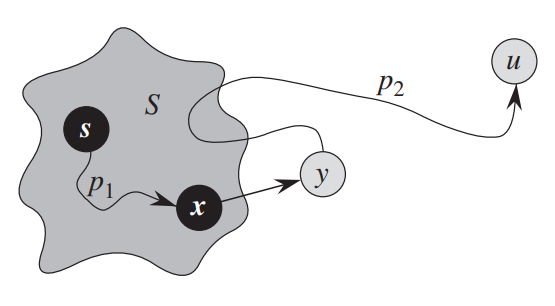
Так как $x$ помечена, то, по предположению индукции, $d_x = l_x$. Раз $(x,y)$ находится на кратчайшем пути, то $l_y=l_x+w$, что в точности равно $d_y=d_x+w$: мы в какой-то момент проводили релаксацию из уже помеченный вершины $x$.
Теперь, может ли быть такое, что $y ne v$? Нет, потому что мы на каждой итерации выбираем вершину с наименьшим $d_v$, а любой вершины дальше $y$ на пути расстояние от $s$ будет больше. Соответственно, $v = y$, и $d_v = d_y = l_y = l_v$, что и требовалось доказать.
#Время работы и реализация
Единственное вариативное место в алгоритме, от которого зависит его сложность — как конкретно искать $v$ с минимальным $d_v$.
#Для плотных графов
Если $m approx n^2$, то на каждой итерации можно просто пройтись по всему массиву и найти $argmin d_v$.
const int maxn = 1e5, inf = 1e9;
vector< pair<int, int> > g[maxn];
int n;

vector<int> dijkstra(int s) {
    vector<int> d(n, inf), a(n, 0);
    d[s] = 0;
    for (int i = 0; i < n; i++) {
        // находим вершину с минимальным d[v] из ещё не помеченных
        int v = -1;
        for (int u = 0; u < n; u++)
            if (!a[u] && (v == -1 || d[u] < d[v]))
                v = u;
        // помечаем её и проводим релаксации вдоль всех исходящих ребер
        a[v] = true;
        for (auto [u, w] : g[v])
            d[u] = min(d[u], d[v] + w);
    }
    return d;
}
Асимптотика такого алгоритма составит $O(n^2)$: на каждой итерации мы находим аргминимум за $O(n)$ и проводим $O(n)$ релаксаций.
Заметим также, что мы можем делать не $n$ итераций а чуть меньше. Во-первых, последнюю итерацию можно никогда не делать (оттуда ничего уже не прорелаксируешь). Во-вторых, можно сразу завершаться, когда мы доходим до недостижимых вершин ($d_v = infty$).
#Для разреженных графов
Если $m approx n$, то минимум можно искать быстрее. Вместо линейного прохода заведем структуру, в которую можно добавлять элементы и искать минимум — например std::set так умеет.
Будем поддерживать в этой структуре пары $(d_v, v)$, при релаксации удаляя старый $(d_u, u)$ и добавляя новый $(d_v + w, u)$, а при нахождении оптимального $v$ просто беря минимум (первый элемент).
Поддерживать массив $a$ нам теперь не нужно: сама структура для нахождения минимума будет играть роль множества ещё не рассмотренных вершин.
vector<int> dijkstra(int s) {
    vector<int> d(n, inf);
    d[root] = 0;
    set< pair<int, int> > q;
    q.insert({0, s});
    while (!q.empty()) {
        int v = q.begin()->second;
        q.erase(q.begin());
        for (auto [u, w] : g[v]) {
            if (d[u] > d[v] + w) {
                q.erase({d[u], u});
                d[u] = d[v] + w;
                q.insert({d[u], u});
            }
        }
    }
    return d;
}
Для каждого ребра нужно сделать два запроса в двоичное дерево, хранящее $O(n)$ элементов, за $O(log n)$ каждый, поэтому асимптотика такого алгоритма составит $O(m log n)$. Заметим, что в случае полных графов это будет равно $O(n^2 log n)$, так что про предыдущий алгоритм забывать не стоит.
#С кучей
Вместо двоичного дерева «правильнее» использовать более специализированную структуру, которая поддерживает именно добавление элементов и нахождение минимума: кучу. Удалять произвольные элементы в ней немного сложнее, поэтому вместо этого будем просто игнорировать все повторные вершины.
vector<int> dijkstra(int s) {
    vector<int> d(n, inf);
    d[root] = 0;
    // объявим очередь с приоритетами для *минимума* (по умолчанию ищется максимум)
    using pair<int, int> Pair;
    priority_queue<Pair, vector<Pair>, greater<Pair>> q;
    q.push({0, s});
    while (!q.empty()) {
        auto [cur_d, v] = q.top();
        q.pop();
        if (cur_d > d[v])
            continue;
        for (auto [u, w] : g[v]) {
            if (d[u] > d[v] + w) {
                d[u] = d[v] + w;
                q.push({d[u], u});
            }
        }
    }
}
На практике вариант с priority_queue немного быстрее.
Помимо обычной двоичной кучи, можно использовать и другие. С теоретической точки зрения, особенно интересна Фибоначчиева куча: у неё все почти все операции кроме работают за $O(1)$, но удаление элементов — за $O(log n)$. Это позволяет облегчить релаксирование до $O(1)$ за счет увеличения времени извлечения минимума до $O(log n)$, что приводит к асимптотике $O(n log n + m)$ вместо $O(m log n)$.
#Восстановление путей
Часто нужно знать не только длины кратчайших путей, но и получить сами пути.
Для этого можно создать массив $p$, в котором в ячейке $p_v$ будет хранится родитель вершины $v$ — вершина, из которой произошла последняя релаксация по ребру $(p_v, v)$.
Обновлять его можно параллельно с массивом $d$. Например, в последней реализации:
if (d[u] > d[v] + w) {
    d[u] = d[v] + w;
    p[u] = v; // <-- кратчайший путь в u идет через ребро (v, u)
    q.push({d[u], u});
}
Для восстановления пути нужно просто пройтись по предкам вершины $v$:
void print_path(int v) {
    while (v != s) {
        cout << v << endl;
        v = p[v];
    }
    cout << s << endl;
}
Обратим внимание, что код распечатает путь в обратном порядке.
Dijkstra’s algorithm to find the shortest path between a and b. It picks the unvisited vertex with the lowest distance, calculates the distance through it to each unvisited neighbor, and updates the neighbor’s distance if smaller. Mark visited (set to red) when done with neighbors. |
|
| Class | Search algorithm Greedy algorithm Dynamic programming[1] |
|---|---|
| Data structure | Graph Usually used with priority queue or heap for optimization[2][3] |
| Worst-case performance |  [3] [3] |
Dijkstra’s algorithm ( DYKE-strəz) is an algorithm for finding the shortest paths between nodes in a weighted graph, which may represent, for example, road networks. It was conceived by computer scientist Edsger W. Dijkstra in 1956 and published three years later.[4][5][6]
The algorithm exists in many variants. Dijkstra’s original algorithm found the shortest path between two given nodes,[6] but a more common variant fixes a single node as the «source» node and finds shortest paths from the source to all other nodes in the graph, producing a shortest-path tree.
For a given source node in the graph, the algorithm finds the shortest path between that node and every other.[7]: 196–206 It can also be used for finding the shortest paths from a single node to a single destination node by stopping the algorithm once the shortest path to the destination node has been determined. For example, if the nodes of the graph represent cities and costs of edge paths represent driving distances between pairs of cities connected by a direct road (for simplicity, ignore red lights, stop signs, toll roads and other obstructions), then Dijkstra’s algorithm can be used to find the shortest route between one city and all other cities. A widely used application of shortest path algorithms is network routing protocols, most notably IS-IS (Intermediate System to Intermediate System) and OSPF (Open Shortest Path First). It is also employed as a subroutine in other algorithms such as Johnson’s.
The Dijkstra algorithm uses labels that are positive integers or real numbers, which are totally ordered. It can be generalized to use any labels that are partially ordered, provided the subsequent labels (a subsequent label is produced when traversing an edge) are monotonically non-decreasing. This generalization is called the generic Dijkstra shortest-path algorithm.[8][9]
Dijkstra’s algorithm uses a data structure for storing and querying partial solutions sorted by distance from the start. Dijkstra’s original algorithm does not use a min-priority queue and runs in time  (where
  is the number of nodes).[10] The idea of this algorithm is also given in Leyzorek et al. 1957. Fredman & Tarjan 1984 propose using a Fibonacci heap min-priority queue to optimize the running time complexity to . This is asymptotically the fastest known single-source shortest-path algorithm for arbitrary directed graphs with unbounded non-negative weights. However, specialized cases (such as bounded/integer weights, directed acyclic graphs etc.) can indeed be improved further as detailed in Specialized variants. Additionally, if preprocessing is allowed algorithms such as contraction hierarchies can be up to seven orders of magnitude faster.
In some fields, artificial intelligence in particular, Dijkstra’s algorithm or a variant of it is known as uniform cost search and formulated as an instance of the more general idea of best-first search.[11]
History[edit]
What is the shortest way to travel from Rotterdam to Groningen, in general: from given city to given city. It is the algorithm for the shortest path, which I designed in about twenty minutes. One morning I was shopping in Amsterdam with my young fiancée, and tired, we sat down on the café terrace to drink a cup of coffee and I was just thinking about whether I could do this, and I then designed the algorithm for the shortest path. As I said, it was a twenty-minute invention. In fact, it was published in ’59, three years later. The publication is still readable, it is, in fact, quite nice. One of the reasons that it is so nice was that I designed it without pencil and paper. I learned later that one of the advantages of designing without pencil and paper is that you are almost forced to avoid all avoidable complexities. Eventually, that algorithm became to my great amazement, one of the cornerstones of my fame.
— Edsger Dijkstra, in an interview with Philip L. Frana, Communications of the ACM, 2001[5]
Dijkstra thought about the shortest path problem when working at the Mathematical Center in Amsterdam in 1956 as a programmer to demonstrate the capabilities of a new computer called ARMAC.[12] His objective was to choose both a problem and a solution (that would be produced by computer) that non-computing people could understand. He designed the shortest path algorithm and later implemented it for ARMAC for a slightly simplified transportation map of 64 cities in the Netherlands (64, so that 6 bits would be sufficient to encode the city number).[5] A year later, he came across another problem from hardware engineers working on the institute’s next computer: minimize the amount of wire needed to connect the pins on the back panel of the machine. As a solution, he re-discovered the algorithm known as Prim’s minimal spanning tree algorithm (known earlier to Jarník, and also rediscovered by Prim).[13][14] Dijkstra published the algorithm in 1959, two years after Prim and 29 years after Jarník.[15][16]
Algorithm[edit]

Illustration of Dijkstra’s algorithm finding a path from a start node (lower left, red) to a goal node (upper right, green) in a robot motion planning problem. Open nodes represent the «tentative» set (aka set of «unvisited» nodes). Filled nodes are the visited ones, with color representing the distance: the greener, the closer. Nodes in all the different directions are explored uniformly, appearing more-or-less as a circular wavefront as Dijkstra’s algorithm uses a heuristic identically equal to 0.
Let the node at which we are starting be called the initial node. Let the distance of node Y be the distance from the initial node to Y. Dijkstra’s algorithm will initially start with infinite distances and will try to improve them step by step.
- Mark all nodes unvisited. Create a set of all the unvisited nodes called the unvisited set.
- Assign to every node a tentative distance value: set it to zero for our initial node and to infinity for all other nodes. During the run of the algorithm, the tentative distance of a node v is the length of the shortest path discovered so far between the node v and the starting node. Since initially no path is known to any other vertex than the source itself (which is a path of length zero), all other tentative distances are initially set to infinity. Set the initial node as current.[17]
- For the current node, consider all of its unvisited neighbors and calculate their tentative distances through the current node. Compare the newly calculated tentative distance to the one currently assigned to the neighbor and assign it the smaller one. For example, if the current node A is marked with a distance of 6, and the edge connecting it with a neighbor B has length 2, then the distance to B through A will be 6 + 2 = 8. If B was previously marked with a distance greater than 8 then change it to 8. Otherwise, the current value will be kept.
- When we are done considering all of the unvisited neighbors of the current node, mark the current node as visited and remove it from the unvisited set. A visited node will never be checked again (this is valid and optimal in connection with the behavior in step 6.: that the next nodes to visit will always be in the order of ‘smallest distance from initial node first’ so any visits after would have a greater distance).
- If the destination node has been marked visited (when planning a route between two specific nodes) or if the smallest tentative distance among the nodes in the unvisited set is infinity (when planning a complete traversal; occurs when there is no connection between the initial node and remaining unvisited nodes), then stop. The algorithm has finished.
- Otherwise, select the unvisited node that is marked with the smallest tentative distance, set it as the new current node, and go back to step 3.
When planning a route, it is actually not necessary to wait until the destination node is «visited» as above: the algorithm can stop once the destination node has the smallest tentative distance among all «unvisited» nodes (and thus could be selected as the next «current»).
Description[edit]
Note: For ease of understanding, this discussion uses the terms intersection, road and map – however, in formal terminology these terms are vertex, edge and graph, respectively.
Suppose you would like to find the shortest path between two intersections on a city map: a starting point and a destination. Dijkstra’s algorithm initially marks the distance (from the starting point) to every other intersection on the map with infinity. This is done not to imply that there is an infinite distance, but to note that those intersections have not been visited yet. Some variants of this method leave the intersections’ distances unlabeled. Now select the current intersection at each iteration. For the first iteration, the current intersection will be the starting point, and the distance to it (the intersection’s label) will be zero. For subsequent iterations (after the first), the current intersection will be a closest unvisited intersection to the starting point (this will be easy to find).
From the current intersection, update the distance to every unvisited intersection that is directly connected to it. This is done by determining the sum of the distance between an unvisited intersection and the value of the current intersection and then relabeling the unvisited intersection with this value (the sum) if it is less than the unvisited intersection’s current value. In effect, the intersection is relabeled if the path to it through the current intersection is shorter than the previously known paths. To facilitate shortest path identification, in pencil, mark the road with an arrow pointing to the relabeled intersection if you label/relabel it, and erase all others pointing to it. After you have updated the distances to each neighboring intersection, mark the current intersection as visited and select an unvisited intersection with minimal distance (from the starting point) – or the lowest label—as the current intersection. Intersections marked as visited are labeled with the shortest path from the starting point to it and will not be revisited or returned to.
Continue this process of updating the neighboring intersections with the shortest distances, marking the current intersection as visited, and moving onto a closest unvisited intersection until you have marked the destination as visited. Once you have marked the destination as visited (as is the case with any visited intersection), you have determined the shortest path to it from the starting point and can trace your way back following the arrows in reverse. In the algorithm’s implementations, this is usually done (after the algorithm has reached the destination node) by following the nodes’ parents from the destination node up to the starting node; that’s why we also keep track of each node’s parent.
This algorithm makes no attempt of direct «exploration» towards the destination as one might expect. Rather, the sole consideration in determining the next «current» intersection is its distance from the starting point. This algorithm therefore expands outward from the starting point, interactively considering every node that is closer in terms of shortest path distance until it reaches the destination. When understood in this way, it is clear how the algorithm necessarily finds the shortest path. However, it may also reveal one of the algorithm’s weaknesses: its relative slowness in some topologies.
Pseudocode[edit]
In the following pseudocode algorithm, dist is an array that contains the current distances from the source to other vertices, i.e. dist[u] is the current distance from the source to the vertex u. The prev array contains pointers to previous-hop nodes on the shortest path from source to the given vertex (equivalently, it is the next-hop on the path from the given vertex to the source). The code u ← vertex in Q with min dist[u], searches for the vertex u in the vertex set Q that has the least dist[u] value. Graph.Edges(u, v) returns the length of the edge joining (i.e. the distance between) the two neighbor-nodes u and v. The variable alt on line 14 is the length of the path from the root node to the neighbor node v if it were to go through u. If this path is shorter than the current shortest path recorded for v, that current path is replaced with this alt path.[7]
A demo of Dijkstra’s algorithm based on Euclidean distance. Red lines are the shortest path covering, i.e., connecting u and prev[u]. Blue lines indicate where relaxing happens, i.e., connecting v with a node u in Q, which gives a shorter path from the source to v.
 1  function Dijkstra(Graph, source):
 2
 3      for each vertex v in Graph.Vertices:
 4          dist[v] ← INFINITY
 5          prev[v] ← UNDEFINED
 6          add v to Q
 7      dist[source] ← 0
 8
 9      while Q is not empty:
10          u ← vertex in Q with min dist[u]
11          remove u from Q
12
13          for each neighbor v of u still in Q:
14              alt ← dist[u] + Graph.Edges(u, v)
15              if alt < dist[v]:
16                  dist[v] ← alt
17                  prev[v] ← u
18
19      return dist[], prev[]
If we are only interested in a shortest path between vertices source and target, we can terminate the search after line 10 if u = target.
Now we can read the shortest path from source to target by reverse iteration:
1  S ← empty sequence
2  u ← target
3  if prev[u] is defined or u = source:          // Do something only if the vertex is reachable
4      while u is defined:                       // Construct the shortest path with a stack S
5          insert u at the beginning of S        // Push the vertex onto the stack
6          u ← prev[u]                           // Traverse from target to source
Now sequence S is the list of vertices constituting one of the shortest paths from source to target, or the empty sequence if no path exists.
A more general problem would be to find all the shortest paths between source and target (there might be several different ones of the same length). Then instead of storing only a single node in each entry of prev[] we would store all nodes satisfying the relaxation condition. For example, if both r and source connect to target and both of them lie on different shortest paths through target (because the edge cost is the same in both cases), then we would add both r and source to prev[target]. When the algorithm completes, prev[] data structure will actually describe a graph that is a subset of the original graph with some edges removed. Its key property will be that if the algorithm was run with some starting node, then every path from that node to any other node in the new graph will be the shortest path between those nodes in the original graph, and all paths of that length from the original graph will be present in the new graph. Then to actually find all these shortest paths between two given nodes we would use a path finding algorithm on the new graph, such as depth-first search.
Using a priority queue[edit]
A min-priority queue is an abstract data type that provides 3 basic operations: add_with_priority(), decrease_priority() and extract_min(). As mentioned earlier, using such a data structure can lead to faster computing times than using a basic queue. Notably, Fibonacci heap[18] or Brodal queue offer optimal implementations for those 3 operations. As the algorithm is slightly different, it is mentioned here, in pseudocode as well:
1  function Dijkstra(Graph, source):
2      dist[source] ← 0                           // Initialization
3
4      create vertex priority queue Q
5
6      for each vertex v in Graph.Vertices:
7          if v ≠ source
8              dist[v] ← INFINITY                 // Unknown distance from source to v
9              prev[v] ← UNDEFINED                // Predecessor of v
10
11         Q.add_with_priority(v, dist[v])
12
13
14     while Q is not empty:                      // The main loop
15         u ← Q.extract_min()                    // Remove and return best vertex
16         for each neighbor v of u:              // Go through all v neighbors of u
17             alt ← dist[u] + Graph.Edges(u, v)
18             if alt < dist[v]:
19                 dist[v] ← alt
20                 prev[v] ← u
21                 Q.decrease_priority(v, alt)
22
23     return dist, prev
Instead of filling the priority queue with all nodes in the initialization phase, it is also possible to initialize it to contain only source; then, inside the if alt < dist[v] block, the decrease_priority() becomes an add_with_priority() operation if the node is not already in the queue.[7]: 198
Yet another alternative is to add nodes unconditionally to the priority queue and to instead check after extraction that it isn’t revisiting, or that no shorter connection was found yet. This can be done by additionally extracting the associated priority p from the queue and only processing further if p == dist[u] inside the while Q is not empty loop. [19]
These alternatives can use entirely array-based priority queues without decrease-key functionality, which have been found to achieve even faster computing times in practice. However, the difference in performance was found to be narrower for denser graphs.[20]
Proof of correctness[edit]
Proof of Dijkstra’s algorithm is constructed by induction on the number of visited nodes.
Invariant hypothesis: For each visited node v, dist[v] is the shortest distance from source to v, and for each unvisited node u, dist[u] is the shortest distance from source to u when traveling via visited nodes only, or infinity if no such path exists. (Note: we do not assume dist[u] is the actual shortest distance for unvisited nodes, while dist[v] is the actual shortest distance)
The base case is when there is just one visited node, namely the initial node source, in which case the hypothesis is trivial.
Next, assume the hypothesis for k-1 visited nodes. Next, we choose u to be the next visited node according to the algorithm. We claim that dist[u] is the shortest distance from source to u.
To prove that claim, we will proceed with a proof by contradiction. If there were a shorter path, then there can be two cases, either the shortest path contains another unvisited node or not.
In the first case, let w be the first unvisited node on the shortest path. By the induction hypothesis, the shortest path from source to u and w through visited node only has cost dist[u] and dist[w] respectively. That means the cost of going from source to u through w has the cost of at least dist[w] + the minimal cost of going from w to u. As the edge costs are positive, the minimal cost of going from w to u is a positive number.
Also dist[u] < dist[w] because the algorithm picked u instead of w.
Now we arrived at a contradiction that dist[u] < dist[w] yet dist[w] + a positive number < dist[u].
In the second case, let w be the last but one node on the shortest path. That means dist[w] + Graph.Edges[w,u] < dist[u]. That is a contradiction because by the time w is visited, it should have set dist[u] to at most dist[w] + Graph.Edges[w,u].
For all other visited nodes v, the induction hypothesis told us dist[v] is the shortest distance from source already, and the algorithm step is not changing that.
After processing u it will still be true that for each unvisited node w, dist[w] will be the shortest distance from source to w using visited nodes only, because if there were a shorter path that doesn’t go by u we would have found it previously, and if there were a shorter path using u we would have updated it when processing u.
After all nodes are visited, the shortest path from source to any node v consists only of visited nodes, therefore dist[v] is the shortest distance.
Running time[edit]
Bounds of the running time of Dijkstra’s algorithm on a graph with edges E and vertices V can be expressed as a function of the number of edges, denoted  , and the number of vertices, denoted , using big-O notation. The complexity bound depends mainly on the data structure used to represent the set Q. In the following, upper bounds can be simplified because is
  for any graph, but that simplification disregards the fact that in some problems, other upper bounds on may hold.
For any data structure for the vertex set Q, the running time is in[2]

where  and
and  are the complexities of the decrease-key and extract-minimum operations in Q, respectively.
The simplest version of Dijkstra’s algorithm stores the vertex set Q as a linked list or array, and edges as an adjacency list or matrix. In this case, extract-minimum is simply a linear search through all vertices in Q, so the running time is  .
.
For sparse graphs, that is, graphs with far fewer than  edges, Dijkstra’s algorithm can be implemented more efficiently by storing the graph in the form of adjacency lists and using a self-balancing binary search tree, binary heap, pairing heap, or Fibonacci heap as a priority queue to implement extracting minimum efficiently. To perform decrease-key steps in a binary heap efficiently, it is necessary to use an auxiliary data structure that maps each vertex to its position in the heap, and to keep this structure up to date as the priority queue Q changes. With a self-balancing binary search tree or binary heap, the algorithm requires

time in the worst case (where  denotes the binary logarithm
  ); for connected graphs this time bound can be simplified to
  . The Fibonacci heap improves this to

When using binary heaps, the average case time complexity is lower than the worst-case: assuming edge costs are drawn independently from a common probability distribution, the expected number of decrease-key operations is bounded by  , giving a total running time of[7]: 199–200

Practical optimizations and infinite graphs[edit]
In common presentations of Dijkstra’s algorithm, initially all nodes are entered into the priority queue. This is, however, not necessary: the algorithm can start with a priority queue that contains only one item, and insert new items as they are discovered (instead of doing a decrease-key, check whether the key is in the queue; if it is, decrease its key, otherwise insert it).[7]: 198 This variant has the same worst-case bounds as the common variant, but maintains a smaller priority queue in practice, speeding up the queue operations.[11]
Moreover, not inserting all nodes in a graph makes it possible to extend the algorithm to find the shortest path from a single source to the closest of a set of target nodes on infinite graphs or those too large to represent in memory. The resulting algorithm is called uniform-cost search (UCS) in the artificial intelligence literature[11][21][22] and can be expressed in pseudocode as
procedure uniform_cost_search(start) is
    node ← start
    frontier ← priority queue containing node only
    expanded ← empty set
    do
        if frontier is empty then
            return failure
        node ← frontier.pop()
        if node is a goal state then
            return solution(node)
        expanded.add(node)
        for each of node's neighbors n do
            if n is not in expanded and not in frontier then
                frontier.add(n)
            else if n is in frontier with higher cost
                replace existing node with n
The complexity of this algorithm can be expressed in an alternative way for very large graphs: when C* is the length of the shortest path from the start node to any node satisfying the «goal» predicate, each edge has cost at least ε, and the number of neighbors per node is bounded by b, then the algorithm’s worst-case time and space complexity are both in O(b1+⌊C* ⁄ ε⌋).[21]
Further optimizations of Dijkstra’s algorithm for the single-target case include bidirectional variants, goal-directed variants such as the A* algorithm (see § Related problems and algorithms), graph pruning to determine which nodes are likely to form the middle segment of shortest paths (reach-based routing), and hierarchical decompositions of the input graph that reduce s–t routing to connecting s and t to their respective «transit nodes» followed by shortest-path computation between these transit nodes using a «highway».[23]
Combinations of such techniques may be needed for optimal practical performance on specific problems.[24]
Specialized variants[edit]
When arc weights are small integers (bounded by a parameter  ), specialized queues which take advantage of this fact can be used to speed up Dijkstra’s algorithm. The first algorithm of this type was Dial’s algorithm (Dial 1969) for graphs with positive integer edge weights, which uses a bucket queue to obtain a running time
  . The use of a Van Emde Boas tree as the priority queue brings the complexity to
  (Ahuja et al. 1990). Another interesting variant based on a combination of a new radix heap and the well-known Fibonacci heap runs in time
  (Ahuja et al. 1990). Finally, the best algorithms in this special case are as follows. The algorithm given by (Thorup 2000) runs in
  time and the algorithm given by (Raman 1997) runs in
  time.
time.
Related problems and algorithms[edit]
The functionality of Dijkstra’s original algorithm can be extended with a variety of modifications. For example, sometimes it is desirable to present solutions which are less than mathematically optimal. To obtain a ranked list of less-than-optimal solutions, the optimal solution is first calculated. A single edge appearing in the optimal solution is removed from the graph, and the optimum solution to this new graph is calculated. Each edge of the original solution is suppressed in turn and a new shortest-path calculated. The secondary solutions are then ranked and presented after the first optimal solution.
Dijkstra’s algorithm is usually the working principle behind link-state routing protocols, OSPF and IS-IS being the most common ones.
Unlike Dijkstra’s algorithm, the Bellman–Ford algorithm can be used on graphs with negative edge weights, as long as the graph contains no negative cycle reachable from the source vertex s. The presence of such cycles means there is no shortest path, since the total weight becomes lower each time the cycle is traversed. (This statement assumes that a «path» is allowed to repeat vertices. In graph theory that is normally not allowed. In theoretical computer science it often is allowed.) It is possible to adapt Dijkstra’s algorithm to handle negative weight edges by combining it with the Bellman-Ford algorithm (to remove negative edges and detect negative cycles); such an algorithm is called Johnson’s algorithm.
The A* algorithm is a generalization of Dijkstra’s algorithm that cuts down on the size of the subgraph that must be explored, if additional information is available that provides a lower bound on the «distance» to the target.
The process that underlies Dijkstra’s algorithm is similar to the greedy process used in Prim’s algorithm. Prim’s purpose is to find a minimum spanning tree that connects all nodes in the graph; Dijkstra is concerned with only two nodes. Prim’s does not evaluate the total weight of the path from the starting node, only the individual edges.
Breadth-first search can be viewed as a special-case of Dijkstra’s algorithm on unweighted graphs, where the priority queue degenerates into a FIFO queue.
The fast marching method can be viewed as a continuous version of Dijkstra’s algorithm which computes the geodesic distance on a triangle mesh.
Dynamic programming perspective[edit]
From a dynamic programming point of view, Dijkstra’s algorithm is a successive approximation scheme that solves the dynamic programming functional equation for the shortest path problem by the Reaching method.[25][26][27]
In fact, Dijkstra’s explanation of the logic behind the algorithm,[28] namely
Problem 2. Find the path of minimum total length between two given nodes
We use the fact that, if


is a paraphrasing of Bellman’s famous Principle of Optimality in the context of the shortest path problem.
Applications[edit]
Least-cost paths are calculated for instance to establish tracks of electricity lines or oil pipelines. The algorithm has also been used to calculate optimal long-distance footpaths in Ethiopia and contrast them with the situation on the ground.[29]
See also[edit]
- A* search algorithm
- Bellman–Ford algorithm
- Euclidean shortest path
- Floyd–Warshall algorithm
- Johnson’s algorithm
- Longest path problem
- Parallel all-pairs shortest path algorithm
Notes[edit]
- ^ Controversial, see Moshe Sniedovich (2006). «Dijkstra’s algorithm revisited: the dynamic programming connexion». Control and Cybernetics. 35: 599–620. and below part.
- ^ a b Cormen et al. 2001
- ^ a b Fredman & Tarjan 1987
- ^ Richards, Hamilton. «Edsger Wybe Dijkstra». A.M. Turing Award. Association for Computing Machinery. Retrieved 16 October 2017.
At the Mathematical Centre a major project was building the ARMAC computer. For its official inauguration in 1956, Dijkstra devised a program to solve a problem interesting to a nontechnical audience: Given a network of roads connecting cities, what is the shortest route between two designated cities?
- ^ a b c Frana, Phil (August 2010). «An Interview with Edsger W. Dijkstra». Communications of the ACM. 53 (8): 41–47. doi:10.1145/1787234.1787249.
- ^ a b Dijkstra, E. W. (1959). «A note on two problems in connexion with graphs» (PDF). Numerische Mathematik. 1: 269–271. doi:10.1007/BF01386390. S2CID 123284777.
- ^ a b c d e Mehlhorn, Kurt; Sanders, Peter (2008). «Chapter 10. Shortest Paths» (PDF). Algorithms and Data Structures: The Basic Toolbox. Springer. doi:10.1007/978-3-540-77978-0. ISBN 978-3-540-77977-3.
- ^ Szcześniak, Ireneusz; Jajszczyk, Andrzej; Woźna-Szcześniak, Bożena (2019). «Generic Dijkstra for optical networks». Journal of Optical Communications and Networking. 11 (11): 568–577. arXiv:1810.04481. doi:10.1364/JOCN.11.000568. S2CID 52958911.
- ^ Szcześniak, Ireneusz; Woźna-Szcześniak, Bożena (2022), Generic Dijkstra: correctness and tractability, arXiv:2204.13547
- ^ Schrijver, Alexander (2012). «On the history of the shortest path problem» (PDF). Documenta Mathematica.
- ^ a b c Felner, Ariel (2011). Position Paper: Dijkstra’s Algorithm versus Uniform Cost Search or a Case Against Dijkstra’s Algorithm. Proc. 4th Int’l Symp. on Combinatorial Search. In a route-finding problem, Felner finds that the queue can be a factor 500–600 smaller, taking some 40% of the running time.
- ^ «ARMAC». Unsung Heroes in Dutch Computing History. 2007. Archived from the original on 13 November 2013.
- ^ Dijkstra, Edsger W., Reflections on «A note on two problems in connexion with graphs (PDF)
- ^ Tarjan, Robert Endre (1983), Data Structures and Network Algorithms, CBMS_NSF Regional Conference Series in Applied Mathematics, vol. 44, Society for Industrial and Applied Mathematics, p. 75,
The third classical minimum spanning tree algorithm was discovered by Jarník and rediscovered by Prim and Dikstra; it is commonly known as Prim’s algorithm.
- ^ Prim, R.C. (1957). «Shortest connection networks and some generalizations» (PDF). Bell System Technical Journal. 36 (6): 1389–1401. Bibcode:1957BSTJ…36.1389P. doi:10.1002/j.1538-7305.1957.tb01515.x. Archived from the original (PDF) on 18 July 2017. Retrieved 18 July 2017.
- ^ V. Jarník: O jistém problému minimálním [About a certain minimal problem], Práce Moravské Přírodovědecké Společnosti, 6, 1930, pp. 57–63. (in Czech)
- ^ Gass, Saul; Fu, Michael (2013). Gass, Saul I; Fu, Michael C (eds.). «Dijkstra’s Algorithm». Encyclopedia of Operations Research and Management Science. Springer. 1. doi:10.1007/978-1-4419-1153-7. ISBN 978-1-4419-1137-7 – via Springer Link.
- ^ Fredman & Tarjan 1984.
- ^ Observe that p < dist[u] cannot ever hold because of the update dist[v] ← alt when updating the queue. See https://cs.stackexchange.com/questions/118388/dijkstra-without-decrease-key for discussion.
- ^ Chen, M.; Chowdhury, R. A.; Ramachandran, V.; Roche, D. L.; Tong, L. (2007). Priority Queues and Dijkstra’s Algorithm – UTCS Technical Report TR-07-54 – 12 October 2007 (PDF). Austin, Texas: The University of Texas at Austin, Department of Computer Sciences.
- ^ a b Russell, Stuart; Norvig, Peter (2009) [1995]. Artificial Intelligence: A Modern Approach (3rd ed.). Prentice Hall. pp. 75, 81. ISBN 978-0-13-604259-4.
- ^ Sometimes also least-cost-first search: Nau, Dana S. (1983). «Expert computer systems» (PDF). Computer. IEEE. 16 (2): 63–85. doi:10.1109/mc.1983.1654302. S2CID 7301753.
- ^ Wagner, Dorothea; Willhalm, Thomas (2007). Speed-up techniques for shortest-path computations. STACS. pp. 23–36.
- ^ Bauer, Reinhard; Delling, Daniel; Sanders, Peter; Schieferdecker, Dennis; Schultes, Dominik; Wagner, Dorothea (2010). «Combining hierarchical and goal-directed speed-up techniques for Dijkstra’s algorithm». J. Experimental Algorithmics. 15: 2.1. doi:10.1145/1671970.1671976. S2CID 1661292.
- ^ Sniedovich, M. (2006). «Dijkstra’s algorithm revisited: the dynamic programming connexion» (PDF). Journal of Control and Cybernetics. 35 (3): 599–620. Online version of the paper with interactive computational modules.
- ^ Denardo, E.V. (2003). Dynamic Programming: Models and Applications. Mineola, NY: Dover Publications. ISBN 978-0-486-42810-9.
- ^ Sniedovich, M. (2010). Dynamic Programming: Foundations and Principles. Francis & Taylor. ISBN 978-0-8247-4099-3.
- ^ Dijkstra 1959, p. 270
- ^ Nyssen, J., Tesfaalem Ghebreyohannes, Hailemariam Meaza, Dondeyne, S., 2020. Exploration of a medieval African map (Aksum, Ethiopia) – How do historical maps fit with topography? In: De Ryck, M., Nyssen, J., Van Acker, K., Van Roy, W., Liber Amicorum: Philippe De Maeyer In Kaart. Wachtebeke (Belgium): University Press: 165-178.
References[edit]
- Cormen, Thomas H.; Leiserson, Charles E.; Rivest, Ronald L.; Stein, Clifford (2001). «Section 24.3: Dijkstra’s algorithm». Introduction to Algorithms (Second ed.). MIT Press and McGraw–Hill. pp. 595–601. ISBN 0-262-03293-7.
- Dial, Robert B. (1969). «Algorithm 360: Shortest-path forest with topological ordering [H]». Communications of the ACM. 12 (11): 632–633. doi:10.1145/363269.363610. S2CID 6754003.
- Fredman, Michael Lawrence; Tarjan, Robert E. (1984). Fibonacci heaps and their uses in improved network optimization algorithms. 25th Annual Symposium on Foundations of Computer Science. IEEE. pp. 338–346. doi:10.1109/SFCS.1984.715934.
- Fredman, Michael Lawrence; Tarjan, Robert E. (1987). «Fibonacci heaps and their uses in improved network optimization algorithms». Journal of the Association for Computing Machinery. 34 (3): 596–615. doi:10.1145/28869.28874. S2CID 7904683.
- Zhan, F. Benjamin; Noon, Charles E. (February 1998). «Shortest Path Algorithms: An Evaluation Using Real Road Networks». Transportation Science. 32 (1): 65–73. doi:10.1287/trsc.32.1.65. S2CID 14986297.
- Leyzorek, M.; Gray, R. S.; Johnson, A. A.; Ladew, W. C.; Meaker, Jr., S. R.; Petry, R. M.; Seitz, R. N. (1957). Investigation of Model Techniques – First Annual Report – 6 June 1956 – 1 July 1957 – A Study of Model Techniques for Communication Systems. Cleveland, Ohio: Case Institute of Technology.
- Knuth, D.E. (1977). «A Generalization of Dijkstra’s Algorithm». Information Processing Letters. 6 (1): 1–5. doi:10.1016/0020-0190(77)90002-3.
- Ahuja, Ravindra K.; Mehlhorn, Kurt; Orlin, James B.; Tarjan, Robert E. (April 1990). «Faster Algorithms for the Shortest Path Problem» (PDF). Journal of the ACM. 37 (2): 213–223. doi:10.1145/77600.77615. hdl:1721.1/47994. S2CID 5499589.
- Raman, Rajeev (1997). «Recent results on the single-source shortest paths problem». SIGACT News. 28 (2): 81–87. doi:10.1145/261342.261352. S2CID 18031586.
- Thorup, Mikkel (2000). «On RAM priority Queues». SIAM Journal on Computing. 30 (1): 86–109. doi:10.1137/S0097539795288246. S2CID 5221089.
- Thorup, Mikkel (1999). «Undirected single-source shortest paths with positive integer weights in linear time». Journal of the ACM. 46 (3): 362–394. doi:10.1145/316542.316548. S2CID 207654795.
External links[edit]
- Oral history interview with Edsger W. Dijkstra, Charles Babbage Institute, University of Minnesota, Minneapolis
- Implementation of Dijkstra’s algorithm using TDD, Robert Cecil Martin, The Clean Code Blog
- 1. Как работает алгоритм Дейкстры
- 2. Пример алгоритма Дейкстры
- 3. Алгоритм Дейкстры. Псевдокод.
- 4. Код для алгоритма Дейкстры
Алгоритм Дейкстры
позволяет нам найти кратчайший путь между любыми двумя вершинами графа.
Он отличается от минимального остовного дерева тем, что кратчайшее расстояние между двумя вершинами может не включать все вершины графа.
Как работает алгоритм Дейкстры
Алгоритм Дейкстры работает на том основании, что любой подпуть B -> D кратчайшего пути A -> D между вершинами A и D также является кратчайшим путем между вершинами B и D.

Дейкстра использовал это свойство в противоположном направлении, т.е. мы переоцениваем расстояние каждой вершины от начальной вершины. Затем мы посещаем каждый узел и его соседей, чтобы найти кратчайший подпуть к этим соседям.
Алгоритм использует «жадный» подход в том смысле, что мы находим следующее лучшее решение, надеясь, что конечный результат является лучшим решением для всей задачи.
Пример алгоритма Дейкстры
Проще начать с примера, а затем подумать об алгоритме.

Алгоритм Дейкстры. Псевдокод.
Нам нужно сохранять расстояние пути каждой вершины. Мы можем сохранить его в массиве размера v, где v — количество вершин.
Нам также хотелось бы получить кратчайший путь, а не только знать его длину. Для этого мы сопоставляем каждую вершину с последней обновленной длиной пути.
Как только алгоритм закончен, мы можем вернуться от вершины назначения к исходной вершине, чтобы найти путь.
Очередь с минимальным приоритетом может использоваться для эффективного получения вершины с наименьшим расстоянием пути.
function dijkstra(G, S) for each vertex V in G distance[V] <- infinite previous[V] <- NULL If V != S, add V to Priority Queue Q distance[S] <- 0 while Q IS NOT EMPTY U <- Extract MIN from Q for each unvisited neighbour V of U tempDistance <- distance[U] + edge_weight(U, V) if tempDistance < distance[V] distance[V] <- tempDistance previous[V] <- U return distance[], previous[]Код для алгоритма Дейкстры
Реализация алгоритма Дейкстры в C ++ приведена ниже. Сложность кода может быть улучшена, но абстракции удобны для связи кода с алгоритмом.
#include <iostream> #include <vector> #define INT_MAX 10000000 using namespace std; void DijkstrasTest(); int main() { DijkstrasTest(); return 0; } class Node; class Edge; void Dijkstras(); vector<Node*>* AdjacentRemainingNodes(Node* node); Node* ExtractSmallest(vector<Node*>& nodes); int Distance(Node* node1, Node* node2); bool Contains(vector<Node*>& nodes, Node* node); void PrintShortestRouteTo(Node* destination); vector<Node*> nodes; vector<Edge*> edges; class Node { public: Node(char id) : id(id), previous(NULL), distanceFromStart(INT_MAX) { nodes.push_back(this); } public: char id; Node* previous; int distanceFromStart; }; class Edge { public: Edge(Node* node1, Node* node2, int distance) : node1(node1), node2(node2), distance(distance) { edges.push_back(this); } bool Connects(Node* node1, Node* node2) { return ( (node1 == this->node1 && node2 == this->node2) || (node1 == this->node2 && node2 == this->node1)); } public: Node* node1; Node* node2; int distance; }; /////////////////// void DijkstrasTest() { Node* a = new Node('a'); Node* b = new Node('b'); Node* c = new Node('c'); Node* d = new Node('d'); Node* e = new Node('e'); Node* f = new Node('f'); Node* g = new Node('g'); Edge* e1 = new Edge(a, c, 1); Edge* e2 = new Edge(a, d, 2); Edge* e3 = new Edge(b, c, 2); Edge* e4 = new Edge(c, d, 1); Edge* e5 = new Edge(b, f, 3); Edge* e6 = new Edge(c, e, 3); Edge* e7 = new Edge(e, f, 2); Edge* e8 = new Edge(d, g, 1); Edge* e9 = new Edge(g, f, 1); a->distanceFromStart = 0; // set start node Dijkstras(); PrintShortestRouteTo(f); } /////////////////// void Dijkstras() { while (nodes.size() > 0) { Node* smallest = ExtractSmallest(nodes); vector<Node*>* adjacentNodes = AdjacentRemainingNodes(smallest); const int size = adjacentNodes->size(); for (int i=0; i<size; ++i) { Node* adjacent = adjacentNodes->at(i); int distance = Distance(smallest, adjacent) + smallest->distanceFromStart; if (distance < adjacent->distanceFromStart) { adjacent->distanceFromStart = distance; adjacent->previous = smallest; } } delete adjacentNodes; } } // Find the node with the smallest distance, // remove it, and return it. Node* ExtractSmallest(vector<Node*>& nodes) { int size = nodes.size(); if (size == 0) return NULL; int smallestPosition = 0; Node* smallest = nodes.at(0); for (int i=1; i<size; ++i) { Node* current = nodes.at(i); if (current->distanceFromStart < smallest->distanceFromStart) { smallest = current; smallestPosition = i; } } nodes.erase(nodes.begin() + smallestPosition); return smallest; } // Return all nodes adjacent to 'node' which are still // in the 'nodes' collection. vector<Node*>* AdjacentRemainingNodes(Node* node) { vector<Node*>* adjacentNodes = new vector<Node*>(); const int size = edges.size(); for(int i=0; i<size; ++i) { Edge* edge = edges.at(i); Node* adjacent = NULL; if (edge->node1 == node) { adjacent = edge->node2; } else if (edge->node2 == node) { adjacent = edge->node1; } if (adjacent && Contains(nodes, adjacent)) { adjacentNodes->push_back(adjacent); } } return adjacentNodes; } // Return distance between two connected nodes int Distance(Node* node1, Node* node2) { const int size = edges.size(); for(int i=0; i<size; ++i) { Edge* edge = edges.at(i); if (edge->Connects(node1, node2)) { return edge->distance; } } return -1; // should never happen } // Does the 'nodes' vector contain 'node' bool Contains(vector<Node*>& nodes, Node* node) { const int size = nodes.size(); for(int i=0; i<size; ++i) { if (node == nodes.at(i)) { return true; } } return false; } /////////////////// void PrintShortestRouteTo(Node* destination) { Node* previous = destination; cout << "Distance from start: " << destination->distanceFromStart << endl; while (previous) { cout << previous->id << " "; previous = previous->previous; } cout << endl; } // these two not needed vector<Edge*>* AdjacentEdges(vector<Edge*>& Edges, Node* node); void RemoveEdge(vector<Edge*>& Edges, Edge* edge); vector<Edge*>* AdjacentEdges(vector<Edge*>& edges, Node* node) { vector<Edge*>* adjacentEdges = new vector<Edge*>(); const int size = edges.size(); for(int i=0; i<size; ++i) { Edge* edge = edges.at(i); if (edge->node1 == node) { cout << "adjacent: " << edge->node2->id << endl; adjacentEdges->push_back(edge); } else if (edge->node2 == node) { cout << "adjacent: " << edge->node1->id << endl; adjacentEdges->push_back(edge); } } return adjacentEdges; } void RemoveEdge(vector<Edge*>& edges, Edge* edge) { vector<Edge*>::iterator it; for (it=edges.begin(); it<edges.end(); ++it) { if (*it == edge) { edges.erase(it); return; } } }