
|
16.2. Статические игры с полной информацией |
633 |
Ситуации, когда в игре существует равновесие в доминирующих стратегиях, достаточно редки. И далеко не во всех играх можно найти решение, отбрасывая строго доминируемые стратегии. Соответствующий пример игры представлен в Таблице 16.8.
Второй игрок выберет стратегию A, если предполагает, что первый выберет стратегию Z; в то же время стратегия B для него предпочтительнее в случае, если первый выберет Y.
Таблица 16.8.
|
A |
B |
C |
|
|
X |
3 |
0 |
1 |
|
2 |
2 |
3 |
|
|
Y |
4 |
6 |
2 |
|
1 |
4 |
2 |
|
|
Z |
7 |
2 |
8 |
|
3 |
1 |
1 |
|
Естественно предположить, что при отсутствии у всех игроков доминирующих стратегий, выбор каждого игрока зависит от ожиданий того, какими будут выборы других. Далее мы рассмотрим концепцию решения, основанную на этой идее.
16.2.4Равновесие по Нэшу
Кроме ситуаций, рассмотренных в предыдущем разделе, бывают ситуации14, которые естественно моделировать, исходя из следующих предположений:
игроки при принятии решений ориентируются на предполагаемые действия партнеров;
ожидания являются равновесными (совпадают с фактически выбранными партнерами действиями).
Если считать, что все игроки рациональны, так что каждый выбирает стратегию, дающую ему наибольший выигрыш при данных ожиданиях, то эти предположения приводят к концепции решения, называемой равновесием Нэша. В равновесии у каждого игрока нет оснований пересматривать свои ожидания.
Формально равновесие Нэша определяется следующим образом.
Определение 90:
Набор стратегий x X является равновесием Нэша15, если
1)стратегия xi каждого игрока является наилучшим для него откликом на ожидаемые им стратегии других игроков xe−i :
ui(xi , xe−i) = max ui(xi, xe−i) i = 1, . . . , n;
xi Xi
14Можно представить себе популяцию игроков типа А (скажем, кошки) и игроков типа Б (скажем, мышки). Игрок типа А при встрече с игроком типа Б имеет оправданные своим или чужим опытом ожидания относительно поведения партнера типа Б, и заранее на них ориентируется (и наоборот). Однако это не единственный тип ситуаций, в которых рассматриваемый подход является адекватным.
15Американский математик Джон Нэш получил Нобелевскую премию по экономике в 1994 г. вместе с Дж. Харшаньи и Р. Зельтеном «за новаторский анализ равновесий в теории некооперативных игр». Концепция равновесия была предложена в следующих статьях: J. F. Nash: Equilibrium Points in N-Person Games,
Proceedings of the National Academy of Sciences of the United States of America 36 (1950): 48–49; J. F. Nash: NonCooperative Games, Annals of Mathematics 54 (1951): 286–295 (рус. пер. Дж. Нэш: Бескоалиционные игры, в кн. Матричные игры, Н. Н. Воробьев (ред.), М.: Физматгиз, 1961: 205–221).
Следует оговориться, что сам Нэш не вводил в определение ожиданий. Исходное определение Нэша совпадает с тем свойством, о котором говорится далее.
|
16.2. Статические игры с полной информацией |
634 |
2) ожидания совпадают с фактически выбираемыми стратегиями:
xe−i = x−i i = 1, . . . , n
Заметим, что при использовании равновесия Нэша для моделирования игровых ситуаций вопросы о том, знают ли игроки цели партнеров, знают ли они о рациональности партнеров, умеют ли их просчитывать, и т. д., отходят на второй план. Способ формирования ожиданий выносится за рамки анализа; здесь важно только то, что ожидания являются равновесными.
Но если при анализе равновесия Нэша не важно, знает ли игрок цели других игроков, то может возникнуть сомнение в правомерности рассмотрения концепции Нэша в контексте игр с полной информацией. Все дело в том, что термин «полная информация» в теории игр имеет довольно узкое значение. Он фактически подразумевает только полноту сведений о типах партнеров (термин «тип игрока», разъясняется в параграфе, посвященном байесовским играм).
Как легко видеть, приведенное определение равновесия Нэша эквивалентно следующему свойству, которое обычно и используется в качестве определения:
Набор стратегий x X является равновесием Нэша, если стратегия xi каждого игрока является наилучшим для него откликом на стратегии других игроков x−i :
ui(xi , x−i) = max ui(xi, x−i) i = 1, . . . , n
xi Xi
Это свойство можно также записать в терминах так называемых функций (отображений) отклика.
Определение 91:
Отображение отклика i-го игрока,
Ri : X−i 7→Xi
сопоставляет каждому набору стратегий других игроков, x−i X−i , множество стратегий i-го игрока, каждая из которых является наилучшим откликом на x−i . Другими словами,
ui(yi, x−i) = max ui(xi, x−i) x−i X−i, yi Ri(x−i) xi Xi
Введение отображений отклика позволяет записать определение равновесия Нэша более компактно: набор стратегий x X является равновесием Нэша, если
xi Ri(x−i) i = 1, . . . , n
Если отклик каждого игрока однозначен (является функцией), то множество равновесий Нэша совпадает с множеством решений системы уравнений:
xi = Ri(x−i) i = 1, . . . , n.
В Таблице 16.8 отображения отклика игроков изображены подчеркиванием выигрышей, соответствующих оптимальным действиям. Равновесие Нэша в данной игре — клетка (B, Y), поскольку выигрыши обоих игроков в ней подчеркнуты.
Проиллюстрируем использование функций отклика на примере игры, в которой игроки имеют континуум стратегий.
|
16.2. Статические игры с полной информацией |
635 |
Игра 5. «Международная торговля»
Две страны одновременно выбирают уровень таможенных пошлин, τi . Объем торговли между странами16, x, зависит от установленных пошлин как
x = 1 − τ1 − τ2
Цель каждой страны — максимизировать доходы ui = τix.
J
Максимизируем выигрыш 1-й страны,
τ1(1 − τ1 − τ2)
по τ1 считая фиксированным уровень пошлины, установленный 2-й страной. Условие первого порядка имеет вид
1 − 2τ1 − τ2 = 0
Поскольку максимизируемая функция строго вогнута, то условие первого порядка соответствует глобальному максимуму.
Условие первого порядка для задачи максимизации выигрыша 2-й страны находится аналогично:
1 − τ1 − 2τ2 = 0
Решив систему из двух линейных уравнений, найдем равновесие Нэша:
τ1 = τ2 = 1/3
Оптимальный отклик 1-й страны на уровень таможенной пошлины, установленной 2-й страной описывается функцией
τ1(τ2) = 1 − τ2
2
Аналогично, функция отклика 2-й страны имеет вид
τ2(τ1) = 1 − τ1 2
Чтобы найти равновесие Нэша, требуется решить систему уравнений
τ1(τ2 ) = τ1 ,
τ2(τ ) = τ .
1 2
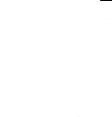
Графически поиск равновесия Нэша показан не Рис. 16.3. Точки, лежащие на кривых оптимального отклика τ1(τ2) и τ2(τ1), характеризуются тем, что в них касательные к кривым безразличия игроков параллельны соответствующей оси координат. Напомним, что кривой безразличия называют множество точек, в которых полезность рассматриваемого индивидуума одна и та же (ui(x) = const). Равновесие находится как точка пересечения кривых отклика.
Преимущество использования концепции равновесия Нэша состоит в том, что можно найти решение и в тех играх, в которых отбрасывание доминируемых стратегий не позволяет этого сделать. Однако сама концепция может показаться более спорной, поскольку опирается на сильные предположения о поведении игроков.
Связь между введенными концепциями решений описывается следующими утверждения-
ми.
16В этой игре мы для упрощения не делаем различия между экспортом и импортом.
|
16.2. Статические игры с полной информацией |
636 |
|
1 |
τ2 |
|||
|
τ1 |
(τ2) |
|||
|
Точка |
равновесия |
|||
|
Нэша |
||||
|
1 |
||||
|
2 |
||||
|
1 |
τ2(τ1) |
|||
|
3 |
||||
|
τ1 |
||||
|
1 |
1 |
1 |
||
|
3 |
2 |
|||
Рис. 16.3. Равновесие Нэша в игре «Международная торговля»
Теорема 151:
Если x = (x1, . . . , xm) — равновесие Нэша в некоторой игре, то ни одна из составляющих его стратегий не может быть отброшена в результате применения процедуры последовательного отбрасывания строго доминируемых стратегий. 
Обратная теорема верна в случае единственности.
Теорема 152:
Если в результате последовательного отбрасывания строго доминируемых стратегий у каждого игрока остается единственная стратегия, xi , то x = (x1, . . . , xm) — равновесие Нэша в этой игре. 
Доказательства этих двух утверждений даны в Приложении B (с. 641). Нам важно здесь, что концепция Нэша не входит в противоречие с идеями рациональности, заложенной в процедуре отбрасывания строго доминируемых стратегий.
По-видимому, естественно считать, что разумно определенное равновесие, не может быть отброшено при последовательном отбрасывании строго доминируемых стратегий. Первую из теорем можно рассматривать как подтверждение того, что концепция Нэша достаточно разумна. Отметим, что данный результат относится только к строгому доминированию. Можно привести пример равновесия Нэша с одной или несколькими слабо доминируемыми стратегиями (см. напр. Таблицу 16.11 на с. 652).
16.2.5Равновесие Нэша в смешанных стратегиях
Нетрудно построить примеры игр, в которых равновесие Нэша отсутствует. Следующая игра представляет пример такой ситуации.
Игра 6. «Инспекция»
В этой игре первый игрок (проверяемый) поставлен перед выбором — платить или не платить подоходный налог. Второй — налоговой инспектор, решает, проверять или не проверять именно этого налогоплательщика. Если инспектор «ловит» недобросовестного налогоплательщика, то взимает в него штраф и получает поощрение по службе, более чем компенсирующее его издержки; в случае же проверки исправного налогоплательщика, инспектор, не получая поощрения, тем не менее несет издержки, связанные с проверкой. Матрица выигрышей представлена в Таблице 16.9.
J

|
16.2. Статические игры с полной информацией |
637 |
||||||||||
|
Таблица 16.9. |
|||||||||||
|
Инспектор |
|||||||||||
|
проверять |
не проверять |
||||||||||
|
нарушать |
1 |
0 |
|||||||||
|
−1 |
1 |
||||||||||
|
Проверяемый |
−1 |
0 |
|||||||||
|
не нарушать |
0 |
0 |
|||||||||
Если инспектор уверен, что налогоплательщик выберет не платить налог, то инспектору выгодно его проверить. С другой стороны, если налогоплательщик уверен, что его проверят, то ему лучше заплатить налог. Аналогичным образом, если инспектор уверен, что налогоплательщик заплатит налог, то инспектору не выгодно его проверять, а если налогоплательщик уверен, что инспектор не станет его проверять, то он предпочтет не платить налог. Оптимальные отклики показаны в таблице подчеркиванием соответствующих выигрышей. Очевидно, что ни одна из клеток не может быть равновесием Нэша, поскольку ни в одной из клеток не подчеркнуты одновременно оба выигрыша.
В подобной игре каждый игрок заинтересован в том, чтобы его партнер не смог угадать, какую именно стратегию он выбрал. Этого можно достигнуть, внеся в выбор стратегии элемент неопределенности.
Те стратегии, которые мы рассматривали раньше, принято называть чистыми стратегиями. Чистые стратегии в статических играх по сути дела совпадают с действиями игроков. Но в некоторых играх естественно ввести в рассмотрение также смешанные стратегии. Под смешанной стратегией понимают распределение вероятностей на чистых стратегиях. В частном случае, когда множество чистых стратегий каждого игрока конечно,
Xi = {x1i , . . . , xni i }
(соответствующая игра называется конечной, ), смешанная стратегия представляется вектором вероятностей соответствующих чистых стратегий:
µi = (µ1i , . . . , µni i )
Обозначим множество смешанных стратегий i-го игрока через Mi :
n o
Mi = µi µki > 0, k = 1, . . . , ni; µ1i + · · · + µni i = 1
Как мы уже отмечали, стандартное предположение теории игр (как и экономической теории) состоит в том, что если выигрыш — случайная величина, то игроки предпочитают действия, которые приносят им наибольший ожидаемый выигрыш. Ожидаемый выигрыш i-го игрока, соответствующий набору смешанных стратегий всех игроков, (µ1, . . . , µm), вычисляется по формуле
|
U(µi, µ−i) = |
n1 |
nm |
|
· · · |
µ1ki · · · µmkm ui(x1ki , . . . , xmkm ) |
|
|
X1 |
X |
|
|
k =1 |
km=1 |
Ожидание рассчитывается в предположении, что игроки выбирают стратегии независимо (в статистическом смысле).
Смешанные стратегии можно представить как результат рандомизации игроком своих действий, то есть как результат их случайного выбора. Например, чтобы выбирать каждую из двух возможных стратегий с одинаковой вероятностью, игрок может подбрасывать монету.

|
16.2. Статические игры с полной информацией |
638 |
Эта интерпретация подразумевает, что выбор стратегии зависит от некоторого сигнала, который сам игрок может наблюдать, а его партнеры — нет17. Например, игрок может выбирать стратегию в зависимости от своего настроения, если ему известно распределение вероятностей его настроений, или от того, с какой ноги он в этот день встал18.
Определение 92:
Набор смешанных стратегий µ = (µ1, . . . , µm) является равновесием Нэша в смешанных стратегиях, если
1)стратегия µi каждого игрока является наилучшим для него откликом на ожидаемые им стратегии других игроков µe−i :
U(µi , µe−i) = max U(µi, µe−i) i = 1, . . . , n;
µi Mi
2) ожидания совпадают с фактически выбираемыми стратегиями:
µe−i = µ−i i = 1, . . . , n.
Заметим, что равновесие Нэша в смешанных стратегиях является обычным равновесием Нэша в так называемом смешанном расширении игры, т. е. игре, чистые стратегии которой являются смешанными стратегиями исходной игры.
Найдем равновесие Нэша в смешанных стратегиях в Игре 16.2.5.
Обозначим через µ вероятность того, что налогоплательщик не платит подоходный налог,
ачерез ν — вероятность того, что налоговой инспектор проверяет налогоплательщика.
Вэтих обозначениях ожидаемый выигрыш налогоплательщика равен
U1(µ, ν) = µ[ν · (−1) + (1 − ν) · 1] + (1 − µ)[ν · 0 + (1 − ν) · 0] =
=µ(1 − 2ν),
аожидаемый выигрыш инспектора равен
U2(µ, ν) = ν[µ · 1 + (1 − µ) · (−1)] + (1 − µ)[µ · 0 + (1 − µ) · 0] = = ν(2µ − 1)
Если вероятность проверки мала (ν < 1/2), то налогоплательщику выгодно не платить налог, т. е. выбрать µ = 1. Если вероятность проверки велика, то налогоплательщику выгодно заплатить налог, т. е. выбрать µ = 0. Если же ν = 1/2, то налогоплательщику все равно, платить налог или нет, он может выбрать любую вероятность µ из интервала [0, 1]. Таким образом, отображение отклика налогоплательщика имеет вид:
|
µ(ν) = |
1, |
если ν < 1/2 |
|
[0, 1] , |
если ν = 1/2 |
|
|
0, |
если ν > 1/2. |
|
Рассуждая аналогичным образом, найдем отклик налогового инспектора:
0, если µ < 1/2
ν(µ) = [0, 1] , если µ = 1/2
1, если µ > 1/2.
17Если сигналы, наблюдаемые игроками, статистически зависимы, то это может помочь игрокам скоординировать свои действия. Это приводит к концепции коррелированного равновесия.
18Впоследствии мы рассмотрим, как можно достигнуть эффекта рандомизации в рамках байесовского равновесия.
![]()
|
16.2. Статические игры с полной информацией |
639 |
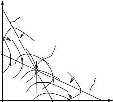
Графики отображений отклика обоих игроков представлены на Рис. 16.4. По осям на этой диаграмме откладываются вероятности (ν и µ соответственно). Они имеют единственную общую точку (1/2, 1/2). Эта точка соответствует равновесию Нэша в смешанных стратегиях. В этом равновесии, как это всегда бывает в равновесиях с невырожденными смешанными стратегиями (то есть в таких равновесиях, в которых ни одна из стратегий не выбирается с вероятностью 1), каждый игрок рандомизирует стратегии, которые обеспечивают ему одинаковую ожидаемую полезность. Вероятности использования соответствующих чистых стратегий, выбранные игроком, определяются не структурой выигрышей данного игрока, а структурой выигрышей его партнера, что может вызвать известные трудности с интерпретацией данного решения.
 ν
ν
ν(µ) 1 

µ(ν)
1
2
µ
Рис. 16.4. Отображения отклика в игре «Инспекция»
В отличие от равновесия в чистых стратегиях, равновесие в смешанных стратегиях в конечных играх существует всегда19, что является следствием следующего общего утверждения.
Теорема 153:
Предположим, что в игре G = hI, {Xi}i I , {ui}i I i у любого игрока множество стратегий Xi непусто, компактно и выпукло, а функция выигрыша ui(·) вогнута по xi и непрерывна. Тогда в игре G существует равновесие Нэша (в чистых стратегиях). 
Существование равновесия Нэша в смешанных стратегиях в играх с конечным числом чистых стратегий является следствием того, что равновесие в смешанных стратегиях является равновесием в чистых стратегиях в смешанном расширении игры.
Теорема 154 (Следствие (Теорема Нэша)):
Равновесие Нэша в смешанных стратегиях существует в любой конечной игре.
Заметим, что существование в игре равновесия в чистых стратегиях не исключает существования равновесия в невырожденных смешанных стратегиях.
Рассмотрим в Игре 16.2.1 «Выбор компьютера» случай, когда выгоды от совместимости значительны, т. е. a < c и b < c. В этом варианте игры два равновесия в чистых стратегиях: (IBM, IBM) и (Mac, Mac). Обозначим µ и ν вероятности выбора компьютера IBM PC первым и вторым игроком соответственно. Ожидаемый выигрыш 1-го игрока равен
U1(µ, ν) = µ[ν · (a + c) + (1 − ν) · a] + (1 − µ)[ν · 0 + (1 − ν) · c] = = µ[ν · 2c − (c − a)] + (1 − ν)c
19Этот результат был доказан Нэшем в статье 1950-го года, цитируемой в сноске 15.
|
16.2. Статические игры с полной информацией |
640 |
а его отклик имеет вид
0,
µ(ν) = [0, 1] ,
1,
Ожидаемый выигрыш 2-го игрока равен
если ν < (c − a)/2c
если ν = (c − a)/2c
если ν > (c − a)/2c.
U2(µ, ν) = ν[µ · c + (1 − µ) · 0] + (1 − ν)[µ · b + (1 − µ) · (b + c)] =
= ν[µ · 2c − (b + c)] + b + (1 − µ)c
а его отклик имеет вид
0,
ν(µ) = [0, 1] ,
1,
если µ < (b + c)/2c
если µ = (b + c)/2c
если µ > (b + c)/2c.
Графики отображений отклика и точки, соответствующие трем равновесиям изображены на Рис. 16.5. Как видно, в рассматриваемой игре кроме двух равновесий в чистых стратегиях имеется одно равновесие в невырожденных смешанных стратегиях. Соответствующие вероятности равны
µ = b + c и ν = c − a
2c 2c
 ν
ν
ν(µ) 1 

µ(ν)
c−a
2c
µ
Рис. 16.5. Случай, когда в игре «Выбор компьютера» существует три равновесия, одно из которых — равновесие в невырожденных смешанных стратегиях
Приложение A
??Теорема повторяется, номер обновляется, ссылки на это приложение нет. Можно поменять местами A и B
Теорема 155:
Предположим, что в игре G = hI, {Xi}i I , {ui0}i I i у любого игрока множество стратегий Xi непусто, компактно и выпукло, а функция выигрыша ui(·) вогнута по xi и непрерывна. Тогда существует равновесие Нэша. 
Доказательство: Докажем, что отображение отклика, Ri(·), каждого игрока полунепрерывно сверху и его значение при каждом x−i X−i непусто и выпукло. Непустота следует из теоремы Вейерштрасса (непрерывная функция на компакте достигает максимума).
16.2. Статические игры с полной информацией
Докажем выпуклость. Пусть z0 , z00 Ri(x−i). Очевидно, что u(z0, x−i) = u(z00, x−i вогнутости по xi функции ui(·) следует, что при α [0, 1]
u(αz0 + (1 − α)z00, x−i) > αu(z0, x−i) + (1 − α)u(z00, x−i) =
= u(z0, x−i) = u(z00, x−i)
Поскольку функция ui(·) достигает максимума в точках z0 и z00 , то строгое неравенство
невозможно. Таким образом,
αz0 + (1 − α)z00 Ri(x−i)
Докажем теперь полунепрерывность сверху отображения Ri(·). Рассмотрим последовательность xni сходящуюся к x¯i и последовательность xn−i сходящуюся к x¯−i , причем xni Ri(xn−i). Заметим, что в силу компактности множеств Xjx¯i Xi и x¯−i X−i . Нам нужно доказать, что x¯i Ri(x¯−i). По определению отображения отклика
u(xni , xn−i) > u(xi, xn−i) xi Xi, n
Из непрерывности функции ui(·) следует, что
u(¯xi, x¯−i) > u(xi, x¯−i) xi Xi
Тем самым, по введенному выше определению отображения отклика, x¯i Ri(x¯−i). Опираясь на доказанные только что свойства отображения Ri(·) и на теорему Какутани,
докажем существование равновесия по Нэшу, то есть такого набора стратегий x X , для
которого выполнено
xi Ri(x−i) i = 1, . . . , n
Определим отображение R(·) из X в X следующим образом:
R(x) = R1(x−1) × · · · × Rn(x−n)
Отметим, что это отображение удовлетворяет тем же свойствам, что и каждое из отображений Ri(·), так как является их декартовым произведением.
Отображение R(·) и множество X удовлетворяют свойствам, которые необходимы для выполнения теоремы Какутани. Таким образом, существует неподвижная точка отображения
R(·):
x R(x )
|
Очевидно, что точка x есть равновесие по Нэшу. |
Приложение B
В этом приложении мы формально докажем утверждения о связи между равновесием Нэша и процедурой последовательного отбрасывания строго доминируемых стратегий.
Сначала определим формально процедуру последовательного отбрасывания строго доминируемых стратегий. Пусть исходная игра задана как
G = hI, {Xi}I , {ui}I i.
Определим последовательность игр {G[t]}t=0,1,2,… , каждая из которых получается из последующей игры отбрасыванием строго доминируемых стратегий. Игры отличаются друг от друга множествами допустимых стратегий:
G[t] = hI, {Xi[t]}I , {ui}I i

|
16.2. Статические игры с полной информацией |
642 |
Процедура начинается с G[0] = G.
Множество допустимых стратегий i-го игрока на шаге t + 1 рассматриваемой процедуры берется равным множеству не доминируемых строго стратегий i-го игрока в игре t-го шага. Множества не доминируемых строго стратегий будем обозначать через NDi (см. определение строго доминируемых стратегий (Определение 89, с. 631)). Формально
NDi = xi Xi  yi Xi : ui(yi, x−i) > ui(xi, x−i) x−i X−i
Таким образом, можно записать шаг рассматриваемой процедуры следующим образом:
Xi[t+1] = NDi[t]
где NDi[t] — множество не доминируемых строго стратегий в игре G[t] .
Приведем теперь доказательства Теорем 151 и 152 (с. 636). Теорема 151 утверждает следующее:
: Если x = (x1, . . . , xm) — равновесие Нэша в некоторой игре, то ни одна из стратегий не может быть отброшена в результате применения процедуры последовательного отбрасывания строго доминируемых стратегий.
Если использовать только что введенные обозначения, то Теорема 151 утверждает, что если x — равновесие Нэша в исходной игре G, то на любом шаге t выполнено
xi Xi[t], i I, t = 1, 2, . . .
или
x X[t], t = 1, 2, . . .
Доказательство (Доказательство Теоремы 151): Пусть есть такой шаг τ , что на нем должна быть отброшена стратегия xi некоторого игрока i I . Предполагается, что на предыдущих шагах ни одна из стратегий не была отброшена:
x X[t], t = 1, . . . , τ.
По определению строгого доминирования существует другая стратегия игрока i, x0i Xi[τ] , которая дает этому игроку в игре G[τ] более высокий выигрыш при любых выборах других
игроков:
ui(x0i, x−i) > ui(xi , x−i) x−i X−[τi]
В том числе, это соотношение должно быть выполнено для x−i , поскольку мы предположили, что стратегии x−i не были отброшены на предыдущих шагах процедуры (x−i X−[τi] ). Значит,
|
ui(xi0, x−i) > ui(xi , x−i) |
|
|
Однако это неравенство противоречит тому, что x — равновесие Нэша. |
|
|
Докажем теперь Теорему 152. Напомним ее формулировку: |
: Если в результате последовательного отбрасывания строго доминируемых стратегий у каждого игрока остается единственная стратегия, xi , то x = (x1, . . . , xm) — равновесие Нэша в этой игре.
Данная теорема относится к случаю, когда в процессе отбрасывания строго доминируемых
стратегий начиная с некоторого шага ¯ остается единственный набор стратегий, , т. е. t x
|
X |
[t] |
= |
x |
, i |
I, |
t = 1, . . . , t.¯ |
|
|
i |
{ i } |
Теорема утверждает, что x является единственным равновесием Нэша исходной игры.
|
16.2. Статические игры с полной информацией |
643 |
Доказательство (Доказательство Теоремы 152): Поскольку, согласно доказанной только что теореме, ни одно из равновесий Нэша не может быть отброшено, нам остается только доказать, что указанный набор стратегий x является равновесием Нэша. Предположим, что это не так. Это означает, что существует стратегия x˜i некоторого игрока i, такая что
ui(xi , x−i) < ui(˜xi, x−i)
По предположению, стратегия x˜i была отброшена на некотором шаге τ , поскольку она не совпадает с xi . Таким образом, существует некоторая строго доминирующая ее стратегия x0i Xi[τ] , так что
ui(x0i, x−i) > ui(˜xi, x−i) x−i X−[τi]
В том числе это неравенство выполнено при x−i = x−i :
ui(x0i, x−i) > ui(˜xi, x−i)
Стратегия x0i не может совпадать со стратегией xi , поскольку в этом случае вышеприведенные неравенства противоречат друг другу. В свою очередь, из этого следует, что должна существовать стратегия x00i , которая доминирует стратегию x0i на некотором шаге τ0 > τ , т. е.
|
u |
(x00 |
, x |
−i |
) > u |
(x0 |
, x |
−i |
) x |
X |
[τ0] |
|
i |
i |
i |
i |
−i |
−i |
В том числе
ui(x00i , x−i) > ui(x0i, x−i)
Можно опять утверждать, что стратегия x00i не может совпадать со стратегией xi , иначе вышеприведенные неравенства противоречили бы друг другу.
Продолжая эти рассуждения, мы получим последовательность шагов τ < τ0 < τ00 < . . .
и соответствующих допустимых стратегий x0i, x00i , x000i , . . ., не совпадающих с xi . Это противо-
|
¯ |
|
|
речит существованию шага t, начиная с которого множества допустимых стратегий состоят |
|
|
i |
|
|
только из x . |
Задачи
/667. Два игрока размещают некоторый объект на плоскости, то есть выбирают его координаты (x, y). Игрок 1 находится в точке (x1 , y1 ), а игрок 2 — в точке (x2 , y2 ). Игрок 1 выбирает координату x, а игрок 2 — координату y. Каждый стремиться, чтобы объект находился как можно ближе к нему. Покажите, что в этой игре у каждого игрока есть строго доминирующая стратегия.
/668. Докажите, что если в некоторой игре у каждого из игроков существует строго доминирующая стратегия, то эти стратегии составляют единственное равновесие Нэша.
/669. Объясните, почему равновесие в доминирующих стратегиях должно быть также равновесием в смысле Нэша. Приведите пример игры, в которой существует равновесие в доминирующих стратегиях, и, кроме того, существуют равновесия Нэша, не совпадающие с равновесием в доминирующих стратегиях.
Найдите в следующих играх все равновесия Нэша.
/670. Игра 16.2.1 (с. 625), выигрыши которой представлены в Таблице ??////??
/671. «Орехи»
Два игрока делят между собой 4 ореха. Каждый делает свою заявку на орехи: xi = 1, 2 или 3. Если x1 + x2 6 4, то каждый получает сколько просил, в противном случае оба не получают ничего.
|
16.2. Статические игры с полной информацией |
644 |
/ 672. Два преподавателя экономического факультета пишут учебник. Качество учебника (q) зависит от их усилий (e1 и e2 соответственно) в соответствии с функцией
q = 2(e1 + e2).
Целевая функция каждого имеет вид
ui = q − ei,
т. е. качество минус усилия. Можно выбрать усилия на уровне 1, 2 или 3.
/ 673. «Третий лишний» Каждый из трех игроков выбирает одну из сторон монеты: «орёл» или «решка». Если
выборы игроков совпали, то каждому выдается по 1 рублю. Если выбор одного из игроков отличается от выбора двух других, то он выплачивает им по 1 рублю.
/ 674. Три игрока выбирают одну из трех альтернатив: A, B или C . Альтернатива выбирается голосованием большинством голосов. Каждый из игроков голосует за одну и только за одну альтернативу. Если ни одна из альтернатив не наберет большинство, то будет выбрана альтернатива A. Выигрыши игроков в зависимости от выбранной альтернативы следующие:
u1(A) = 2, u2(A) = 0, u3(A) = 1,
u1(B) = 1, u2(B) = 2, u3(B) = 0,
u1(C) = 0, u2(C) = 1, u3(C) = 2.
/675. Формируются два избирательных блока, которые будут претендовать на места в законодательном собрании города N-ска. Каждый из блоков может выбрать одну из трех ориентаций: «левая» (L), «правая» (R) и «экологическая» (E). Каждая из ориентаций может привлечь 50, 30 и 20% избирателей соответственно. Известно, что если интересующая их ориентация не представлена на выборах, то избиратели из соответствующей группы не будут голосовать. Если блоки выберут разные ориентации, то каждый получит соответствующую долю голосов. Если блоки выберут одну и ту же ориентацию, то голоса соответствующей группы избирателей разделятся поровну между ними. Цель каждого блока — получить наибольшее количество голосов.
/676. Два игрока размещают точку на плоскости. Один игрок выбирает абсциссу, другой —
ординату. Их выигрыши заданы функциями:
а) ux(x, y) = −x2 + x(y + a) + y2 , uy(x, y) = −y2 + y(x + b) + x2 ,
б) ux(x, y) = −x2 − 2ax(y + 1) + y2 , uy(x, y) = −y2 + 2by(x + 1) + x2 , в) ux(x, y) = −x − y/x + 1/2y2 , uy(x, y) = −y − x/y + 1/2x2 ,
(a, b — коэффициенты).
/677. «Мороженщики на пляже»
Два мороженщика в жаркий день продают на пляже мороженое. Пляж можно представить как единичный отрезок. Мороженщики выбирают, в каком месте пляжа им находиться, т. е. выбирают координату xi [0, 1]. Покупатели равномерно рассредоточены по пляжу и покупают мороженое у ближайшего к ним продавца. Если x1 < x2 , то первый обслуживают (x1 + x2)/2 долю пляжа, а второй — 1 − (x1 + x2)/2. Если мороженщики расположатся в одной и той же точке (x1 = x2 ), покупатели поровну распределятся между ними. Каждый мороженщик стремиться обслуживать как можно большую долю пляжа.
/ 678. «Аукцион» Рассмотрите аукцион, подобный описанному в Игре 16.2.2, при условии, что выигравший
аукцион игрок платит названную им цену.
/ 679. Проанализируйте Игру 16.2.1 «Выбор компьютера» (с. 624) и найдите ответы на следующие вопросы:

|
16.2. Статические игры с полной информацией |
645 |
а) При каких условиях на параметры a, b и c будет существовать равновесие в доминирующих стратегиях? Каким будет это равновесие?
б) При каких условиях на параметры будет равновесием Нэша исход, когда оба выбирают IBM? Когда это равновесие единственно? Может ли оно являться также равновесием в доминирующих стратегиях?
/ 680. Каждый из двух соседей по подъезду выбирает, будет он подметать подъезд раз в неделю или нет. Пусть каждый оценивает выгоду для себя от двойной чистоты в a > 0 денежных единиц, выгоду от одинарной чистоты — в b > 0 единиц, от неубранного подъезда — в 0, а свои затраты на личное участие в уборке — в c > 0. При каких соотношениях между a, b и c в игре сложатся равновесия вида: (0) никто не убирает, (1) один убирает, (2) оба убирают?
/ 681. Предположим, что в некоторой игре двух игроков, каждый из которых имеет 2 стратегии, существует единственное равновесие Нэша. Покажите, что в этой игре хотя бы у одного из игроков есть доминирующая стратегия.
/ 682. Каждый из двух игроков (i = 1, 2) имеет по 3 стратегии: a, b, c и x, y, z соответственно. Взяв свое имя как бесконечную последовательность символов типа иваниваниван. . . , задайте выигрыши первого игрока так: u1(a, x) = «и», u1(a, y) = «в», u1(a, z) = «а», u1(b, x) = «н», u1(b, y) = «и», u1(b, z) = «в», u1(c, x) = «а», u1(c, y) = «н», u1(c, z) = «и». Подставьте вместо каждой буквы имени ее номер в алфавите, для чего воспользуйтесь Таблицей 16.10. Аналогично используя фамилию, задайте выигрыши второго игрока, u2(·).
1)Есть ли в Вашей игре доминирующие и строго доминирующие стратегии? Если есть, то образуют ли они равновесие в доминирующих стратегиях?
2)Каким будет результат последовательного отбрасывания строго доминируемых страте-
гий?
3)Найдите равновесия Нэша этой игры.
Таблица 16.10.
|
0 |
1 |
2 |
3 |
4 |
5 |
6 |
7 |
8 |
9 |
|
|
0 |
а |
б |
в |
г |
д |
е |
ё |
ж |
з |
|
|
1 |
и |
й |
к |
л |
м |
н |
о |
п |
р |
с |
|
2 |
т |
у |
ф |
х |
ц |
ч |
ш |
щ |
ъ |
ы |
|
3 |
ь |
э |
ю |
я |
/683. Составьте по имени, фамилии и отчеству матричную игру трех игроков, у каждого из которых по 2 стратегии. Ответьте на вопросы предыдущей задачи.
/684. Заполните пропущенные выигрыши в следующей таблице так, чтобы в получившейся игре. . .
(0)не было ни одного равновесия Нэша,
|
(1) |
было одно равновесие Нэша, |
1 |
? |
|
|
? |
2 |
|||
|
(2) |
было два равновесия Нэша, |
|||
|
? |
0 |
|||
|
(3) |
было три равновесия Нэша, |
|||
|
4 |
? |
(4)было четыре равновесия Нэша.
/685. 1) Объясните, почему в любом равновесии Нэша выигрыш i-го игрока не может быть меньше, чем
min max ui(xi, x−i).
x−i X−i xi Xi
2) Объясните, почему в любом равновесии Нэша выигрыш i-го игрока не может быть
|
меньше, чем |
|||||
|
max min |
u |
(x |
, x |
−i |
). |
|
xi Xi x−i X−i |
i |
i |
Что такое теория игр?
Теория игр — это область математики, которая занимается проблемами, в которых решение принимают несколько участников, называемых игроками. Название предполагает, что это связано с настольными или компьютерными играми. Первоначально теория игр использовалась для анализа стратегий настольных игр; однако в настоящее время он используется для решения множества реальных проблем.
В математической игре выигрыш игрока определяется не только его собственным выбором стратегии, но и стратегиями, выбранными другими игроками. Поэтому важно предвидеть действия других игроков. Теория игр пытается проанализировать оптимальную стратегию для нескольких типов игр.

Настольные игры
Кедр101
Теория некооперативных игр
Подраздел теории игр — это теория некооперативных игр. Это поле имеет дело с проблемами, при которых игроки не могут сотрудничать и должны принимать решение о своей стратегии, не имея возможности обсудить с другими игроками.
В теории некооперативных игр есть два типа игр:
- В одновременных играх оба игрока принимают решение одновременно.
- В последовательных играх игроки должны действовать по порядку. Знают ли они, какие стратегии выбрали предыдущие игроки, зависит от игры. Если да, то это называется игрой с полной информацией, в противном случае — игрой с неполной информацией.

Джон Форбс Нэш мл.
Эльке Ветциг (Elya) / CC BY-SA (http://creativecommons.org/licenses/by-sa/3.0/)
Джон Форбс Нэш мл.
Джон Форбс Нэш-младший был американским математиком, который жил с 1928 по 2015 год. Он был исследователем в Принстонском университете. Его работа была в основном в области теории игр, в которую он внес значительный вклад. В 1994 году он получил Нобелевскую премию по экономике за свои применения теории игр в экономике. Равновесие по Нэшу является частью всей теории равновесия, предложенной Нэшем.
Пример: дилемма заключенного
Дилемма заключенного — один из самых известных примеров некооперативной теории игр. Двое друзей арестованы за преступление. Полиция самостоятельно спрашивает их, сделали ли они это или нет. Если оба солгут и скажут, что нет, и они оба получат три года тюрьмы, потому что у полиции мало улик против них.
Если оба скажут правду о своей виновности, каждый получит по семь лет. Если один говорит правду, а другой лжет, то тот, кто говорит правду, получает один год тюрьмы, а другой — десять. Эта игра отображается в таблице ниже. В матрице стратегии игрока A отображаются вертикально, а стратегии игрока B — горизонтально. Выплата x, y означает, что игрок A получает x, а игрок B — y.
|
Ложь |
Говорить правду |
|
|
Ложь |
3,3 |
10,1 |
|
Говорить правду |
1,10 |
7,7 |

Джулия Форсайт
Что такое равновесие по Нэшу и как его найти?
Определение равновесия по Нэшу является результатом игры, в которой ни один из игроков не хочет менять стратегию, если другие этого не сделают. Дилемма заключенного имеет одно равновесие по Нэшу, а именно 7,7, что соответствует обоим игрокам, говорящим правду. Если игрок А станет лгать, а игрок Б будет говорить правду, игрок А получит 10 лет тюрьмы, так что он не переключится. То же самое и с игроком B.
Похоже, что 3,3 — лучшее решение, чем 7,7. Однако 3,3 не является равновесием по Нэшу. Если у игроков остается 3,3, тогда, если игрок переключается с лжи на правду, он сокращает свой штраф до 1 года, если другой остается с ложью.
Игры с множественными равновесиями Нэша
Игра может иметь несколько равновесий по Нэшу. Пример показан в таблице ниже. В этом примере выплаты положительные. Так что большее число лучше.
|
Осталось |
Правильно |
|
|
верхний |
5,4 |
2,3 |
|
Дно |
1,7 |
4,9 |
В этой игре оба (вверху, слева) и (внизу, справа) являются равновесиями по Нэшу. Если A и B выберут (Top, Left), то A может переключиться на Bottom, но это уменьшит его выигрыш с 5 до 1. Игрок B может переключаться слева направо, но это уменьшит его выигрыш с 4 до 3.
Если игроки находятся в (Снизу, справа), игрок A может переключиться, но затем он снижает свой выигрыш с 4 до 2, а игрок B может только уменьшить свой выигрыш с 9 до 7.
Игры без равновесия по Нэшу
Помимо наличия одного или нескольких равновесий по Нэшу, игра также может не иметь равновесия по Нэшу. Пример игры, в которой нет равновесия по Нэшу, показан в таблице ниже.
|
Осталось |
Правильно |
|
|
верхний |
5,4 |
2,6 |
|
Дно |
4,6 |
5,3 |
Если игроки окажутся в (Сверху, Слева), игрок Б захочет переключиться на Право. Если они попадают в (верхнее, правое), игрок А хочет переключиться на нижний. Более того, если они окажутся в (Снизу, слева), игрок А предпочел бы занять Вверху, а если они попали в (Снизу, справа), игроку Б было бы лучше выбрать Слева. Следовательно, ни один из четырех вариантов не является равновесием по Нэшу.
Смешанные стратегии
До сих пор мы рассматривали только чистые стратегии, то есть игрок выбирает только одну стратегию. Однако игрок также может разработать стратегию, в которой он выбирает каждую стратегию с определенной вероятностью. Например, он играет влево с вероятностью 0,4 и вправо с вероятностью 0,6.
Джон Форбс Нэш-младший доказал, что в каждой игре есть хотя бы одно равновесие по Нэшу, когда разрешена смешанная стратегия. Таким образом, при использовании смешанных стратегий в приведенной выше игре, в которой, как говорилось, не было равновесия по Нэшу, оно действительно будет. Однако определение этого равновесия по Нэшу — очень сложная задача.
Равновесия Нэша на практике
Примером равновесия по Нэшу на практике является закон, который никто не нарушит. Например красный и зеленый светофоры. Когда две машины едут на перекресток с разных сторон, есть четыре варианта. Оба едут, оба останавливаются, машина 1 едет, а машина 2 останавливается, или машина 1 останавливается, а машина 2 едет. Мы можем смоделировать решения водителей как игру со следующей матрицей выплат.
|
Водить машину |
Стоп |
|
|
Водить машину |
-5, -5 |
2,1 |
|
Стоп |
1,2 |
-1, -1 |
Если оба игрока будут вести машину, они разобьются, что является худшим исходом для обоих. Если оба останавливаются, они ждут, пока никого нет за рулем, что хуже, чем ждать, пока за рулем другой человек. Следовательно, обе ситуации, когда едет ровно одна машина, являются равновесиями по Нэшу. В реальном мире такую ситуацию создают светофоры.

Светофор
Рафал Почтарски
Подобную игру можно использовать для моделирования множества других ситуаций. Например посетители в больнице. Для больного плохо, если к нему приходит слишком много людей. Лучше, когда никто не приходит, потому что тогда он сможет отдохнуть. Однако тогда он будет один. Поэтому лучше всего, когда приходит только один посетитель. Это обеспечивается установкой не более одного посетителя.
Заключительные замечания о равновесии по Нэшу
Как мы видели, равновесие по Нэшу относится к ситуации, когда ни один игрок не хочет переключаться на другую стратегию. Однако это не означает, что нет лучших результатов. На практике множество ситуаций можно смоделировать как игру. Когда игроки действуют в соответствии со стратегией равновесия Нэша, никто не захочет нарушать его решение.
© 2020 Джон
| Nash equilibrium | |
|---|---|
| A solution concept in game theory | |
| Relationship | |
| Subset of | Rationalizability, Epsilon-equilibrium, Correlated equilibrium |
| Superset of | Evolutionarily stable strategy, Subgame perfect equilibrium, Perfect Bayesian equilibrium, Trembling hand perfect equilibrium, Stable Nash equilibrium, Strong Nash equilibrium, Cournot equilibrium |
| Significance | |
| Proposed by | John Forbes Nash Jr. |
| Used for | All non-cooperative games |
In game theory, the Nash equilibrium, named after the mathematician John Nash, is the most common way to define the solution of a non-cooperative game involving two or more players. In a Nash equilibrium, each player is assumed to know the equilibrium strategies of the other players, and no one has anything to gain by changing only one’s own strategy.[1] The principle of Nash equilibrium dates back to the time of Cournot, who in 1838 applied it to competing firms choosing outputs.[2]
If each player has chosen a strategy – an action plan based on what has happened so far in the game – and no one can increase one’s own expected payoff by changing one’s strategy while the other players keep theirs unchanged, then the current set of strategy choices constitutes a Nash equilibrium.
If two players Alice and Bob choose strategies A and B, (A, B) is a Nash equilibrium if Alice has no other strategy available that does better than A at maximizing her payoff in response to Bob choosing B, and Bob has no other strategy available that does better than B at maximizing his payoff in response to Alice choosing A. In a game in which Carol and Dan are also players, (A, B, C, D) is a Nash equilibrium if A is Alice’s best response to (B, C, D), B is Bob’s best response to (A, C, D), and so forth.
Nash showed that there is a Nash equilibrium for every finite game (see Strategy (game theory)).
Applications[edit]
Game theorists use Nash equilibrium to analyze the outcome of the strategic interaction of several decision makers. In a strategic interaction, the outcome for each decision-maker depends on the decisions of the others as well as their own. The simple insight underlying Nash’s idea is that one cannot predict the choices of multiple decision makers if one analyzes those decisions in isolation. Instead, one must ask what each player would do taking into account what the player expects the others to do. Nash equilibrium requires that one’s choices be consistent: no players wish to undo their decision given what the others are deciding.
The concept has been used to analyze hostile situations such as wars and arms races[3] (see prisoner’s dilemma), and also how conflict may be mitigated by repeated interaction (see tit-for-tat). It has also been used to study to what extent people with different preferences can cooperate (see battle of the sexes), and whether they will take risks to achieve a cooperative outcome (see stag hunt). It has been used to study the adoption of technical standards,[citation needed] and also the occurrence of bank runs and currency crises (see coordination game). Other applications include traffic flow (see Wardrop’s principle), how to organize auctions (see auction theory), the outcome of efforts exerted by multiple parties in the education process,[4] regulatory legislation such as environmental regulations (see tragedy of the commons),[5] natural resource management,[6] analysing strategies in marketing,[7] even penalty kicks in football (see matching pennies),[8] energy systems, transportation systems, evacuation problems[9] and wireless communications.[10]
History[edit]
Nash equilibrium is named after American mathematician John Forbes Nash Jr. The same idea was used in a particular application in 1838 by Antoine Augustin Cournot in his theory of oligopoly.[11] In Cournot’s theory, each of several firms choose how much output to produce to maximize its profit. The best output for one firm depends on the outputs of the others. A Cournot equilibrium occurs when each firm’s output maximizes its profits given the output of the other firms, which is a pure-strategy Nash equilibrium. Cournot also introduced the concept of best response dynamics in his analysis of the stability of equilibrium. Cournot did not use the idea in any other applications, however, or define it generally.
The modern concept of Nash equilibrium is instead defined in terms of mixed strategies, where players choose a probability distribution over possible pure strategies (which might put 100% of the probability on one pure strategy; such pure strategies are a subset of mixed strategies). The concept of a mixed-strategy equilibrium was introduced by John von Neumann and Oskar Morgenstern in their 1944 book The Theory of Games and Economic Behavior, but their analysis was restricted to the special case of zero-sum games. They showed that a mixed-strategy Nash equilibrium will exist for any zero-sum game with a finite set of actions.[12] The contribution of Nash in his 1951 article «Non-Cooperative Games» was to define a mixed-strategy Nash equilibrium for any game with a finite set of actions and prove that at least one (mixed-strategy) Nash equilibrium must exist in such a game. The key to Nash’s ability to prove existence far more generally than von Neumann lay in his definition of equilibrium. According to Nash, «an equilibrium point is an n-tuple such that each player’s mixed strategy maximizes his payoff if the strategies of the others are held fixed. Thus each player’s strategy is optimal against those of the others.» Putting the problem in this framework allowed Nash to employ the Kakutani fixed-point theorem in his 1950 paper to prove existence of equilibria. His 1951 paper used the simpler Brouwer fixed-point theorem for the same purpose.[13]
Game theorists have discovered that in some circumstances Nash equilibrium makes invalid predictions or fails to make a unique prediction. They have proposed many solution concepts (‘refinements’ of Nash equilibria) designed to rule out implausible Nash equilibria. One particularly important issue is that some Nash equilibria may be based on threats that are not ‘credible’. In 1965 Reinhard Selten proposed subgame perfect equilibrium as a refinement that eliminates equilibria which depend on non-credible threats. Other extensions of the Nash equilibrium concept have addressed what happens if a game is repeated, or what happens if a game is played in the absence of complete information. However, subsequent refinements and extensions of Nash equilibrium share the main insight on which Nash’s concept rests: the equilibrium is a set of strategies such that each player’s strategy is optimal given the choices of the others.
Definitions[edit]
Nash equilibrium[edit]
A strategy profile is a set of strategies, one for each player. Informally, a strategy profile is a Nash equilibrium if no player can do better by unilaterally changing their strategy. To see what this means, imagine that each player is told the strategies of the others. Suppose then that each player asks themselves: «Knowing the strategies of the other players, and treating the strategies of the other players as set in stone, can I benefit by changing my strategy?»
If any player could answer «Yes», then that set of strategies is not a Nash equilibrium. But if every player prefers not to switch (or is indifferent between switching and not) then the strategy profile is a Nash equilibrium. Thus, each strategy in a Nash equilibrium is a best response to the other players’ strategies in that equilibrium.[14]
Formally, let  be the set of all possible strategies for player
  , where
  . Let
. Let  be a strategy profile, a set consisting of one strategy for each player, where
  denotes the
  strategies of all the players except . Let
  be player i’s payoff as a function of the strategies. The strategy profile
  is a Nash equilibrium if

A game can have more than one Nash equilibrium. Even if the equilibrium is unique, it might be weak: a player might be indifferent among several strategies given the other players’ choices. It is unique and called a strict Nash equilibrium if the inequality is strict so one strategy is the unique best response:

Note that the strategy set can be different for different players, and its elements can be a variety of mathematical objects. Most simply, a player might choose between two strategies, e.g.  Or, the strategy set might be a finite set of conditional strategies responding to other players, e.g.
  Or, it might be an infinite set, a continuum or unbounded, e.g.
  such that
  is a non-negative real number. Nash’s existence proofs assume a finite strategy set, but the concept of Nash equilibrium does not require it.
The Nash equilibrium may sometimes appear non-rational in a third-person perspective. This is because a Nash equilibrium is not necessarily Pareto optimal.
Nash equilibrium may also have non-rational consequences in sequential games because players may «threaten» each other with threats they would not actually carry out. For such games the subgame perfect Nash equilibrium may be more meaningful as a tool of analysis.
Strict/weak equilibrium[edit]
Suppose that in the Nash equilibrium, each player asks themselves: «Knowing the strategies of the other players, and treating the strategies of the other players as set in stone, would I suffer a loss by changing my strategy?»
If every player’s answer is «Yes», then the equilibrium is classified as a strict Nash equilibrium.[15]
If instead, for some player, there is exact equality between the strategy in Nash equilibrium and some other strategy that gives exactly the same payout (i.e. this player is indifferent between switching and not), then the equilibrium is classified as a weak Nash equilibrium.
A game can have a pure-strategy or a mixed-strategy Nash equilibrium. (In the latter a pure strategy is chosen stochastically with a fixed probability).
Nash’s existence theorem[edit]
Nash proved that if mixed strategies (where a player chooses probabilities of using various pure strategies) are allowed, then every game with a finite number of players in which each player can choose from finitely many pure strategies has at least one Nash equilibrium, which might be a pure strategy for each player or might be a probability distribution over strategies for each player.
Nash equilibria need not exist if the set of choices is infinite and non-compact. An example is a game where two players simultaneously name a number and the player naming the larger number wins. Another example is where each of two players chooses a real number strictly less than 5 and the winner is whoever has the biggest number; no biggest number strictly less than 5 exists (if the number could equal 5, the Nash equilibrium would have both players choosing 5 and tying the game). However, a Nash equilibrium exists if the set of choices is compact with each player’s payoff continuous in the strategies of all the players.[16]
Examples[edit]
Coordination game[edit]
| Player 1 strategy | Player 2 strategy | |
|---|---|---|
| Player 2 adopts strategy A | Player 2 adopts strategy B | |
| Player 1 adopts strategy A |
4 4 |
3 1 |
| Player 1 adopts strategy B |
1 3 |
2 2 |
The coordination game is a classic two-player, two-strategy game, as shown in the example payoff matrix to the right. There are two pure-strategy equilibria, (A,A) with payoff 4 for each player and (B,B) with payoff 2 for each. The combination (B,B) is a Nash equilibrium because if either player unilaterally changes his strategy from B to A, his payoff will fall from 2 to 1.
| Player 1 strategy | Player 2 strategy | |
|---|---|---|
| Hunt stag | Hunt rabbit | |
| Hunt stag |
2 2 |
1 0 |
| Hunt rabbit |
0 1 |
1 1 |
A famous example of a coordination game is the stag hunt. Two players may choose to hunt a stag or a rabbit, the stag providing more meat (4 utility units, 2 for each player) than the rabbit (1 utility unit). The caveat is that the stag must be cooperatively hunted, so if one player attempts to hunt the stag, while the other hunts the rabbit, the stag hunter will totally fail, for a payoff of 0, whereas the rabbit-hunter will succeed, for a payoff of 1. The game has two equilibria, (stag, stag) and (rabbit, rabbit), because a player’s optimal strategy depends on his expectation on what the other player will do. If one hunter trusts that the other will hunt the stag, he should hunt the stag; however if he thinks the other will hunt the rabbit, he too will hunt the rabbit. This game is used as an analogy for social cooperation, since much of the benefit that people gain in society depends upon people cooperating and implicitly trusting one another to act in a manner corresponding with cooperation.
Driving on a road against an oncoming car, and having to choose either to swerve on the left or to swerve on the right of the road, is also a coordination game. For example, with payoffs 10 meaning no crash and 0 meaning a crash, the coordination game can be defined with the following payoff matrix:
| Player 1 strategy | Player 2 strategy | |
|---|---|---|
| Drive on the left | Drive on the right | |
| Drive on the left |
10 10 |
0 0 |
| Drive on the right |
0 0 |
10 10 |
In this case there are two pure-strategy Nash equilibria, when both choose to either drive on the left or on the right. If we admit mixed strategies (where a pure strategy is chosen at random, subject to some fixed probability), then there are three Nash equilibria for the same case: two we have seen from the pure-strategy form, where the probabilities are (0%, 100%) for player one, (0%, 100%) for player two; and (100%, 0%) for player one, (100%, 0%) for player two respectively. We add another where the probabilities for each player are (50%, 50%).
Network traffic[edit]
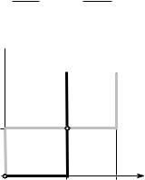
Sample network graph. Values on edges are the travel time experienced by a «car» traveling down that edge.  is the number of cars traveling via that edge.
An application of Nash equilibria is in determining the expected flow of traffic in a network. Consider the graph on the right. If we assume that there are «cars» traveling from A to D, what is the expected distribution of traffic in the network?
This situation can be modeled as a «game», where every traveler has a choice of 3 strategies and where each strategy is a route from A to D (one of ABD, ABCD, or ACD). The «payoff» of each strategy is the travel time of each route. In the graph on the right, a car travelling via ABD experiences travel time of  , where is the number of cars traveling on edge AB. Thus, payoffs for any given strategy depend on the choices of the other players, as is usual. However, the goal, in this case, is to minimize travel time, not maximize it. Equilibrium will occur when the time on all paths is exactly the same. When that happens, no single driver has any incentive to switch routes, since it can only add to their travel time. For the graph on the right, if, for example, 100 cars are travelling from A to D, then equilibrium will occur when 25 drivers travel via ABD, 50 via ABCD, and 25 via ACD. Every driver now has a total travel time of 3.75 (to see this, note that a total of 75 cars take the AB edge, and likewise, 75 cars take the CD edge).
Notice that this distribution is not, actually, socially optimal. If the 100 cars agreed that 50 travel via ABD and the other 50 through ACD, then travel time for any single car would actually be 3.5, which is less than 3.75. This is also the Nash equilibrium if the path between B and C is removed, which means that adding another possible route can decrease the efficiency of the system, a phenomenon known as Braess’s paradox.
Competition game[edit]
| Player 1 strategy | Player 2 strategy | |||
|---|---|---|---|---|
| Choose «0» | Choose «1» | Choose «2» | Choose «3» | |
| Choose «0» | 0, 0 | 2, −2 | 2, −2 | 2, −2 |
| Choose «1» | −2, 2 | 1, 1 | 3, −1 | 3, −1 |
| Choose «2» | −2, 2 | −1, 3 | 2, 2 | 4, 0 |
| Choose «3» | −2, 2 | −1, 3 | 0, 4 | 3, 3 |
This can be illustrated by a two-player game in which both players simultaneously choose an integer from 0 to 3 and they both win the smaller of the two numbers in points. In addition, if one player chooses a larger number than the other, then they have to give up two points to the other.
This game has a unique pure-strategy Nash equilibrium: both players choosing 0 (highlighted in light red). Any other strategy can be improved by a player switching their number to one less than that of the other player. In the adjacent table, if the game begins at the green square, it is in player 1’s interest to move to the purple square and it is in player 2’s interest to move to the blue square. Although it would not fit the definition of a competition game, if the game is modified so that the two players win the named amount if they both choose the same number, and otherwise win nothing, then there are 4 Nash equilibria: (0,0), (1,1), (2,2), and (3,3).
Nash equilibria in a payoff matrix[edit]
There is an easy numerical way to identify Nash equilibria on a payoff matrix. It is especially helpful in two-person games where players have more than two strategies. In this case formal analysis may become too long. This rule does not apply to the case where mixed (stochastic) strategies are of interest. The rule goes as follows: if the first payoff number, in the payoff pair of the cell, is the maximum of the column of the cell and if the second number is the maximum of the row of the cell — then the cell represents a Nash equilibrium.
| Player 1 strategy | Player 2 strategy | ||
|---|---|---|---|
| Option A | Option B | Option C | |
| Option A | 0, 0 | 25, 40 | 5, 10 |
| Option B | 40, 25 | 0, 0 | 5, 15 |
| Option C | 10, 5 | 15, 5 | 10, 10 |
We can apply this rule to a 3×3 matrix:
Using the rule, we can very quickly (much faster than with formal analysis) see that the Nash equilibria cells are (B,A), (A,B), and (C,C). Indeed, for cell (B,A), 40 is the maximum of the first column and 25 is the maximum of the second row. For (A,B), 25 is the maximum of the second column and 40 is the maximum of the first row; the same applies for cell (C,C). For other cells, either one or both of the duplet members are not the maximum of the corresponding rows and columns.
This said, the actual mechanics of finding equilibrium cells is obvious: find the maximum of a column and check if the second member of the pair is the maximum of the row. If these conditions are met, the cell represents a Nash equilibrium. Check all columns this way to find all NE cells. An N×N matrix may have between 0 and N×N pure-strategy Nash equilibria.
Stability[edit]
The concept of stability, useful in the analysis of many kinds of equilibria, can also be applied to Nash equilibria.
A Nash equilibrium for a mixed-strategy game is stable if a small change (specifically, an infinitesimal change) in probabilities for one player leads to a situation where two conditions hold:
- the player who did not change has no better strategy in the new circumstance
- the player who did change is now playing with a strictly worse strategy.
If these cases are both met, then a player with the small change in their mixed strategy will return immediately to the Nash equilibrium. The equilibrium is said to be stable. If condition one does not hold then the equilibrium is unstable. If only condition one holds then there are likely to be an infinite number of optimal strategies for the player who changed.
In the «driving game» example above there are both stable and unstable equilibria. The equilibria involving mixed strategies with 100% probabilities are stable. If either player changes their probabilities slightly, they will be both at a disadvantage, and their opponent will have no reason to change their strategy in turn. The (50%,50%) equilibrium is unstable. If either player changes their probabilities (which would neither benefit or damage the expectation of the player who did the change, if the other player’s mixed strategy is still (50%,50%)), then the other player immediately has a better strategy at either (0%, 100%) or (100%, 0%).
Stability is crucial in practical applications of Nash equilibria, since the mixed strategy of each player is not perfectly known, but has to be inferred from statistical distribution of their actions in the game. In this case unstable equilibria are very unlikely to arise in practice, since any minute change in the proportions of each strategy seen will lead to a change in strategy and the breakdown of the equilibrium.
The Nash equilibrium defines stability only in terms of unilateral deviations. In cooperative games such a concept is not convincing enough. Strong Nash equilibrium allows for deviations by every conceivable coalition.[17] Formally, a strong Nash equilibrium is a Nash equilibrium in which no coalition, taking the actions of its complements as given, can cooperatively deviate in a way that benefits all of its members.[18] However, the strong Nash concept is sometimes perceived as too «strong» in that the environment allows for unlimited private communication. In fact, strong Nash equilibrium has to be Pareto efficient. As a result of these requirements, strong Nash is too rare to be useful in many branches of game theory. However, in games such as elections with many more players than possible outcomes, it can be more common than a stable equilibrium.
A refined Nash equilibrium known as coalition-proof Nash equilibrium (CPNE)[17] occurs when players cannot do better even if they are allowed to communicate and make «self-enforcing» agreement to deviate. Every correlated strategy supported by iterated strict dominance and on the Pareto frontier is a CPNE.[19] Further, it is possible for a game to have a Nash equilibrium that is resilient against coalitions less than a specified size, k. CPNE is related to the theory of the core.
Finally in the eighties, building with great depth on such ideas Mertens-stable equilibria were introduced as a solution concept. Mertens stable equilibria satisfy both forward induction and backward induction. In a game theory context stable equilibria now usually refer to Mertens stable equilibria.
Occurrence[edit]
If a game has a unique Nash equilibrium and is played among players under certain conditions, then the NE strategy set will be adopted. Sufficient conditions to guarantee that the Nash equilibrium is played are:
- The players all will do their utmost to maximize their expected payoff as described by the game.
- The players are flawless in execution.
- The players have sufficient intelligence to deduce the solution.
- The players know the planned equilibrium strategy of all of the other players.
- The players believe that a deviation in their own strategy will not cause deviations by any other players.
- There is common knowledge that all players meet these conditions, including this one. So, not only must each player know the other players meet the conditions, but also they must know that they all know that they meet them, and know that they know that they know that they meet them, and so on.
Where the conditions are not met[edit]
Examples of game theory problems in which these conditions are not met:
- The first condition is not met if the game does not correctly describe the quantities a player wishes to maximize. In this case there is no particular reason for that player to adopt an equilibrium strategy. For instance, the prisoner’s dilemma is not a dilemma if either player is happy to be jailed indefinitely.
- Intentional or accidental imperfection in execution. For example, a computer capable of flawless logical play facing a second flawless computer will result in equilibrium. Introduction of imperfection will lead to its disruption either through loss to the player who makes the mistake, or through negation of the common knowledge criterion leading to possible victory for the player. (An example would be a player suddenly putting the car into reverse in the game of chicken, ensuring a no-loss no-win scenario).
- In many cases, the third condition is not met because, even though the equilibrium must exist, it is unknown due to the complexity of the game, for instance in Chinese chess.[20] Or, if known, it may not be known to all players, as when playing tic-tac-toe with a small child who desperately wants to win (meeting the other criteria).
- The criterion of common knowledge may not be met even if all players do, in fact, meet all the other criteria. Players wrongly distrusting each other’s rationality may adopt counter-strategies to expected irrational play on their opponents’ behalf. This is a major consideration in «chicken» or an arms race, for example.
Where the conditions are met[edit]
In his Ph.D. dissertation, John Nash proposed two interpretations of his equilibrium concept, with the objective of showing how equilibrium points can be connected with observable phenomenon.
(…) One interpretation is rationalistic: if we assume that players are rational, know the full structure of the game, the game is played just once, and there is just one Nash equilibrium, then players will play according to that equilibrium.
This idea was formalized by R. Aumann and A. Brandenburger, 1995, Epistemic Conditions for Nash Equilibrium, Econometrica, 63, 1161-1180 who interpreted each player’s mixed strategy as a conjecture about the behaviour of other players and have shown that if the game and the rationality of players is mutually known and these conjectures are commonly known, then the conjectures must be a Nash equilibrium (a common prior assumption is needed for this result in general, but not in the case of two players. In this case, the conjectures need only be mutually known).
A second interpretation, that Nash referred to by the mass action interpretation, is less demanding on players:
[i]t is unnecessary to assume that the participants have full knowledge of the total structure of the game, or the ability and inclination to go through any complex reasoning processes. What is assumed is that there is a population of participants for each position in the game, which will be played throughout time by participants drawn at random from the different populations. If there is a stable average frequency with which each pure strategy is employed by the average member of the appropriate population, then this stable average frequency constitutes a mixed strategy Nash equilibrium.
For a formal result along these lines, see Kuhn, H. and et al., 1996, «The Work of John Nash in Game Theory,» Journal of Economic Theory, 69, 153–185.
Due to the limited conditions in which NE can actually be observed, they are rarely treated as a guide to day-to-day behaviour, or observed in practice in human negotiations. However, as a theoretical concept in economics and evolutionary biology, the NE has explanatory power. The payoff in economics is utility (or sometimes money), and in evolutionary biology is gene transmission; both are the fundamental bottom line of survival. Researchers who apply games theory in these fields claim that strategies failing to maximize these for whatever reason will be competed out of the market or environment, which are ascribed the ability to test all strategies. This conclusion is drawn from the «stability» theory above. In these situations the assumption that the strategy observed is actually a NE has often been borne out by research.[21]
NE and non-credible threats[edit]

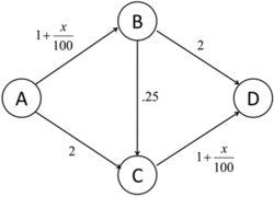
Extensive and Normal form illustrations that show the difference between SPNE and other NE. The blue equilibrium is not subgame perfect because player two makes a non-credible threat at 2(2) to be unkind (U).
The Nash equilibrium is a superset of the subgame perfect Nash equilibrium. The subgame perfect equilibrium in addition to the Nash equilibrium requires that the strategy also is a Nash equilibrium in every subgame of that game. This eliminates all non-credible threats, that is, strategies that contain non-rational moves in order to make the counter-player change their strategy.
The image to the right shows a simple sequential game that illustrates the issue with subgame imperfect Nash equilibria. In this game player one chooses left(L) or right(R), which is followed by player two being called upon to be kind (K) or unkind (U) to player one, However, player two only stands to gain from being unkind if player one goes left. If player one goes right the rational player two would de facto be kind to her/him in that subgame. However, The non-credible threat of being unkind at 2(2) is still part of the blue (L, (U,U)) Nash equilibrium. Therefore, if rational behavior can be expected by both parties the subgame perfect Nash equilibrium may be a more meaningful solution concept when such dynamic inconsistencies arise.
Proof of existence[edit]
Proof using the Kakutani fixed-point theorem[edit]
Nash’s original proof (in his thesis) used Brouwer’s fixed-point theorem (e.g., see below for a variant). We give a simpler proof via the Kakutani fixed-point theorem, following Nash’s 1950 paper (he credits David Gale with the observation that such a simplification is possible).
To prove the existence of a Nash equilibrium, let  be the best response of player i to the strategies of all other players.

Here,  , where
  , is a mixed-strategy profile in the set of all mixed strategies and
  is the payoff function for player i. Define a set-valued function
  such that
  . The existence of a Nash equilibrium is equivalent to
  having a fixed point.
Kakutani’s fixed point theorem guarantees the existence of a fixed point if the following four conditions are satisfied.
 is compact, convex, and nonempty.
- is nonempty.
- is upper hemicontinuous
- is convex.

Condition 1. is satisfied from the fact that  is a simplex and thus compact. Convexity follows from players’ ability to mix strategies. is nonempty as long as players have strategies.
Condition 2. and 3. are satisfied by way of Berge’s maximum theorem. Because is continuous and compact,  is non-empty and upper hemicontinuous.
Condition 4. is satisfied as a result of mixed strategies. Suppose  , then
  . i.e. if two strategies maximize payoffs, then a mix between the two strategies will yield the same payoff.
Therefore, there exists a fixed point in and a Nash equilibrium.[22]
When Nash made this point to John von Neumann in 1949, von Neumann famously dismissed it with the words, «That’s trivial, you know. That’s just a fixed-point theorem.» (See Nasar, 1998, p. 94.)
Alternate proof using the Brouwer fixed-point theorem[edit]
We have a game  where
where  is the number of players and
  is the action set for the players. All of the action sets
  are finite. Let
  denote the set of mixed strategies for the players. The finiteness of the s ensures the compactness of
  .
.
We can now define the gain functions. For a mixed strategy  , we let the gain for player on action
  be
be

The gain function represents the benefit a player gets by unilaterally changing their strategy. We now define  where
where

for  . We see that

Next we define:

It is easy to see that each  is a valid mixed strategy in
  . It is also easy to check that each is a continuous function of
  , and hence
  is a continuous function. As the cross product of a finite number of compact convex sets, is also compact and convex. Applying the Brouwer fixed point theorem to and we conclude that has a fixed point in , call it
  . We claim that is a Nash equilibrium in
  . For this purpose, it suffices to show that

This simply states that each player gains no benefit by unilaterally changing their strategy, which is exactly the necessary condition for a Nash equilibrium.
Now assume that the gains are not all zero. Therefore,  and such that
  . Note then that

So let

Also we shall denote  as the gain vector indexed by actions in . Since is the fixed point we have:
![{displaystyle {begin{aligned}sigma ^{*}=f(sigma ^{*})&Rightarrow sigma _{i}^{*}=f_{i}(sigma ^{*})\&Rightarrow sigma _{i}^{*}={frac {g_{i}(sigma ^{*})}{sum _{ain A_{i}}g_{i}(sigma ^{*})(a)}}\[6pt]&Rightarrow sigma _{i}^{*}={frac {1}{C}}left(sigma _{i}^{*}+{text{Gain}}_{i}(sigma ^{*},cdot )right)\[6pt]&Rightarrow Csigma _{i}^{*}=sigma _{i}^{*}+{text{Gain}}_{i}(sigma ^{*},cdot )\&Rightarrow left(C-1right)sigma _{i}^{*}={text{Gain}}_{i}(sigma ^{*},cdot )\&Rightarrow sigma _{i}^{*}=left({frac {1}{C-1}}right){text{Gain}}_{i}(sigma ^{*},cdot ).end{aligned}}}](https://wikimedia.org/api/rest_v1/media/math/render/svg/556e976617ee74da95e980547e8d4f7a1aef701c)
Since  we have that
  is some positive scaling of the vector
  . Now we claim that

To see this, we first note that if then this is true by definition of the gain function. Now assume that  . By our previous statements we have that

and so the left term is zero, giving us that the entire expression is  as needed.
So we finally have that

where the last inequality follows since is a non-zero vector. But this is a clear contradiction, so all the gains must indeed be zero. Therefore, is a Nash equilibrium for as needed.
Computing Nash equilibria[edit]
If a player A has a dominant strategy  then there exists a Nash equilibrium in which A plays . In the case of two players A and B, there exists a Nash equilibrium in which A plays and B plays a best response to . If is a strictly dominant strategy, A plays in all Nash equilibria. If both A and B have strictly dominant strategies, there exists a unique Nash equilibrium in which each plays their strictly dominant strategy.
In games with mixed-strategy Nash equilibria, the probability of a player choosing any particular (so pure) strategy can be computed by assigning a variable to each strategy that represents a fixed probability for choosing that strategy. In order for a player to be willing to randomize, their expected payoff for each (pure) strategy should be the same. In addition, the sum of the probabilities for each strategy of a particular player should be 1. This creates a system of equations from which the probabilities of choosing each strategy can be derived.[14]
Examples[edit]
| Strategy | Player B plays H | Player B plays T |
|---|---|---|
| Player A plays H | −1, +1 | +1, −1 |
| Player A plays T | +1, −1 | −1, +1 |
In the matching pennies game, player A loses a point to B if A and B play the same strategy and wins a point from B if they play different strategies. To compute the mixed-strategy Nash equilibrium, assign A the probability  of playing H and
  of playing T, and assign B the probability
  of playing H and
  of playing T.
![{displaystyle {begin{aligned}&mathbb {E} [{text{payoff for A playing H}}]=(-1)q+(+1)(1-q)=1-2q\&mathbb {E} [{text{payoff for A playing T}}]=(+1)q+(-1)(1-q)=2q-1\&mathbb {E} [{text{payoff for A playing H}}]=mathbb {E} [{text{payoff for A playing T}}]implies 1-2q=2q-1implies q={frac {1}{2}}\&mathbb {E} [{text{payoff for B playing H}}]=(+1)p+(-1)(1-p)=2p-1\&mathbb {E} [{text{payoff for B playing T}}]=(-1)p+(+1)(1-p)=1-2p\&mathbb {E} [{text{payoff for B playing H}}]=mathbb {E} [{text{payoff for B playing T}}]implies 2p-1=1-2pimplies p={frac {1}{2}}\end{aligned}}}](https://wikimedia.org/api/rest_v1/media/math/render/svg/2eb56208b46327ad1d4aba30ca5f8d81a22a043f)
Thus, a mixed-strategy Nash equilibrium in this game is for each player to randomly choose H or T with  and
and  .
.
Oddness of equilibrium points[edit]
In 1971, Robert Wilson came up with the Oddness Theorem, [23] which says that «almost all» finite games have a finite and odd number of Nash equilibria. In 1993, Harsanyi published an alternative proof of the result.[24] «Almost all» here means that any game with an infinite or even number of equilibria is very special in the sense that if its payoffs were even slightly randomly perturbed, with probability one it would have an odd number of equilibria instead.
| Strategy | Player B votes Yes | Player B votes No |
|---|---|---|
| Player A votes Yes | 1, 1 | 0, 0 |
| Player A votes No | 0, 0 | 0, 0 |
The prisoner’s dilemma, for example, has one equilibrium, while the battle of the sexes has three— two pure and one mixed, and this remains true even if the payoffs change slightly. The free money game is an example of a «special» game with an even number of equilibria. In it, two players have to both vote «yes» rather than «no» to get a reward and the votes are simultaneous. There are two pure-strategy Nash equilibria, (yes, yes) and (no, no), and no mixed strategy equilibria, because the strategy «yes» weakly dominates «no». «Yes» is as good as «no» regardless of the other player’s action, but if there is any chance the other player chooses «yes» then «yes» is the best reply. Under a small random perturbation of the payoffs, however, the probability that any two payoffs would remain tied, whether at 0 or some other number, is vanishingly small, and the game would have either one or three equilibria instead.
See also[edit]
- Adjusted winner procedure – Method of fairly dividing property
- Complementarity theory – type of mathematical optimization problem
- Conflict resolution research
- Cooperation – Groups working or acting together
- Equilibrium selection
- Evolutionarily stable strategy – Solution concept in game theory
- Glossary of game theory – List of definitions of terms and concepts used in game theory
- Hotelling’s law – Observation in economics
- Manipulated Nash equilibrium
- Mexican standoff – Type of confrontation
- Minimax theorem – Gives conditions that guarantee the max–min inequality is also an equality
- Mutual assured destruction – Doctrine of military strategy
- Extended Mathematical Programming for Equilibrium Problems
- Optimum contract and par contract – Bridge scoring terms in the card game contract bridge
- Self-confirming equilibrium
- Solution concept – Formal rule for predicting how a game will be played
- Stackelberg competition – Economic model
- Wardrop’s principle – Major theorist of traffic flow equilibrium
References[edit]
- ^ Osborne, Martin J.; Rubinstein, Ariel (12 Jul 1994). A Course in Game Theory. Cambridge, MA: MIT. p. 14. ISBN 9780262150415.
- ^ Kreps D.M. (1987) «Nash Equilibrium.» In: Palgrave Macmillan (eds) The New Palgrave Dictionary of Economics. Palgrave Macmillan, London.
- ^ Schelling, Thomas, The Strategy of Conflict, copyright 1960, 1980, Harvard University Press, ISBN 0-674-84031-3.
- ^ De Fraja, G.; Oliveira, T.; Zanchi, L. (2010). «Must Try Harder: Evaluating the Role of Effort in Educational Attainment». Review of Economics and Statistics. 92 (3): 577. doi:10.1162/REST_a_00013. hdl:2108/55644. S2CID 57072280.
- ^ Ward, H. (1996). «Game Theory and the Politics of Global Warming: The State of Play and Beyond». Political Studies. 44 (5): 850–871. doi:10.1111/j.1467-9248.1996.tb00338.x. S2CID 143728467.,
- ^ Thorpe, Robert B.; Jennings, Simon; Dolder, Paul J. (2017). «Risks and benefits of catching pretty good yield in multispecies mixed fisheries». ICES Journal of Marine Science. 74 (8): 2097–2106. doi:10.1093/icesjms/fsx062.,
- ^ «Marketing Lessons from Dr. Nash — Andrew Frank». 2015-05-25. Retrieved 2015-08-30.
- ^ Chiappori, P. -A.; Levitt, S.; Groseclose, T. (2002). «Testing Mixed-Strategy Equilibria when Players Are Heterogeneous: The Case of Penalty Kicks in Soccer» (PDF). American Economic Review. 92 (4): 1138. CiteSeerX 10.1.1.178.1646. doi:10.1257/00028280260344678.
- ^ Djehiche, B.; Tcheukam, A.; Tembine, H. (2017). «A Mean-Field Game of Evacuation in Multilevel Building». IEEE Transactions on Automatic Control. 62 (10): 5154–5169. doi:10.1109/TAC.2017.2679487. ISSN 0018-9286. S2CID 21850096.
- ^ Djehiche, Boualem; Tcheukam, Alain; Tembine, Hamidou (2017-09-27). «Mean-Field-Type Games in Engineering». AIMS Electronics and Electrical Engineering. 1: 18–73. arXiv:1605.03281. doi:10.3934/ElectrEng.2017.1.18. S2CID 16055840.
- ^ Cournot A. (1838) Researches on the Mathematical Principles of the Theory of Wealth
- ^ J. Von Neumann, O. Morgenstern, Theory of Games and Economic Behavior, copyright 1944, 1953, Princeton University Press
- ^ Carmona, Guilherme; Podczeck, Konrad (2009). «On the Existence of Pure Strategy Nash Equilibria in Large Games» (PDF). Journal of Economic Theory. 144 (3): 1300–1319. doi:10.1016/j.jet.2008.11.009. hdl:10362/11577. SSRN 882466.
- ^ a b von Ahn, Luis. «Preliminaries of Game Theory» (PDF). Archived from the original (PDF) on 2011-10-18. Retrieved 2008-11-07.
- ^ «Nash Equilibria». hoylab.cornell.edu. Retrieved 2019-12-08.
- ^ MIT OpenCourseWare. 6.254: Game Theory with Engineering Applications, Spring 2010. Lecture 6: Continuous and Discontinuous Games.
- ^ a b B. D. Bernheim; B. Peleg; M. D. Whinston (1987), «Coalition-Proof Equilibria I. Concepts», Journal of Economic Theory, 42 (1): 1–12, doi:10.1016/0022-0531(87)90099-8.
- ^ Aumann, R. (1959). «Acceptable points in general cooperative n-person games». Contributions to the Theory of Games. Vol. IV. Princeton, N.J.: Princeton University Press. ISBN 978-1-4008-8216-8.
- ^ D. Moreno; J. Wooders (1996), «Coalition-Proof Equilibrium» (PDF), Games and Economic Behavior, 17 (1): 80–112, doi:10.1006/game.1996.0095, hdl:10016/4408.
- ^ T. L. Turocy, B. Von Stengel, Game Theory, copyright 2001, Texas A&M University, London School of Economics, pages 141-144. Nash proved that a perfect NE exists for this type of finite extensive form game[citation needed] – it can be represented as a strategy complying with his original conditions for a game with a NE. Such games may not have unique NE, but at least one of the many equilibrium strategies would be played by hypothetical players having perfect knowledge of all 10150 game trees[citation needed].
- ^ J. C. Cox, M. Walker, Learning to Play Cournot Duoploy Strategies Archived 2013-12-11 at the Wayback Machine, copyright 1997, Texas A&M University, University of Arizona, pages 141-144
- ^ Fudenburg, Drew; Tirole, Jean (1991). Game Theory. MIT Press. ISBN 978-0-262-06141-4.
- ^ Wilson, Robert (1971-07-01). «Computing Equilibria of N-Person Games». SIAM Journal on Applied Mathematics. 21 (1): 80–87. doi:10.1137/0121011. ISSN 0036-1399.
- ^ Harsanyi, J. C. (1973-12-01). «Oddness of the Number of Equilibrium Points: A New Proof». International Journal of Game Theory. 2 (1): 235–250. doi:10.1007/BF01737572. ISSN 1432-1270. S2CID 122603890.
Bibliography[edit]
Game theory textbooks[edit]
- Binmore, Ken (2007), Playing for Real: A Text on Game Theory, Oxford University Press, ISBN 978-0195300574.
- Dixit, Avinash, Susan Skeath and David Reiley. Games of Strategy. W.W. Norton & Company. (Third edition in 2009.) An undergraduate text.
- Dutta, Prajit K. (1999), Strategies and games: theory and practice, MIT Press, ISBN 978-0-262-04169-0. Suitable for undergraduate and business students.
- Fudenberg, Drew and Jean Tirole (1991) Game Theory MIT Press.
- Gibbons, Robert (1992), Game Theory for Applied Economists, Princeton University Press (July 13, 1992), ISBN 978-0-691-00395-5. Lucid and detailed introduction to game theory in an explicitly economic context.
- Morgenstern, Oskar and John von Neumann (1947) The Theory of Games and Economic Behavior Princeton University Press.
- Myerson, Roger B. (1997), Game Theory: Analysis of Conflict, Harvard University Press, ISBN 978-0-674-34116-6
- Osborne, Martin (2004), An Introduction to Game Theory, Oxford University Press, ISBN 978-0-19-512895-6.
- Papayoanou, Paul (2010), Game Theory for Business: A Primer in Strategic Gaming, Probabilistic Publishing, ISBN 978-0964793873
- Rubinstein, Ariel; Osborne, Martin J. (1994), A Course in Game Theory, MIT Press, ISBN 978-0-262-65040-3. A modern introduction at the graduate level.
- Shoham, Yoav; Leyton-Brown, Kevin (2009), Multiagent Systems: Algorithmic, Game-Theoretic, and Logical Foundations, New York: Cambridge University Press, ISBN 978-0-521-89943-7. A comprehensive reference from a computational perspective; see Chapter 3. Downloadable free online.
Original Nash papers[edit]
- Nash, John (1950) «Equilibrium points in n-person games» Proceedings of the National Academy of Sciences 36(1):48-49.
- Nash, John (1951) «Non-Cooperative Games» The Annals of Mathematics 54(2):286-295.
Other references[edit]
- Mehlmann, A. (2000) The Game’s Afoot! Game Theory in Myth and Paradox, American Mathematical Society.
- Nasar, Sylvia (1998), A Beautiful Mind, Simon & Schuster.
- Aviad Rubinstein: «Hardness of Approximation Between P and NP», ACM, ISBN 978-1-947487-23-9 (May 2019), DOI: https://doi.org/10.1145/3241304 . # Explains the Nash Equilibrium is a hard problem in computation.
External links[edit]
- «Nash theorem (in game theory)», Encyclopedia of Mathematics, EMS Press, 2001 [1994]
- Complete Proof of Existence of Nash Equilibria
- Simplified Form and Related Results Archived 2021-07-31 at the Wayback Machine