Алгоритм Дейкстры. Разбор Задач
Время на прочтение
7 мин
Количество просмотров 36K
Поиск оптимального пути в графе. Такая задача встречается довольно часто и в повседневной жизни, и в мире технологий. Справиться с такими вызовами помогает подход, который должен быть в арсенале каждого программиста — алгоритм Дейкстры.
Если вы хотите найти ответить на вопросы, чем этот алгоритм лучше BFS (поиска в ширину), при каких условиях алгоритм применим, и какие теоретические и практические задачи можно с его помощью решать, читайте далее.
Введение
Алгоритм Дейкстры работает на ориентированных (с некоторыми дополнениями и на неориентированных) графах, и призван искать кратчайшие пути между заданной вершиной и всеми остальными вершинами в графе.
Как правило, граф обозначают как набор вершин и рёбер  где число рёбер может быть задано
  , а вершин числом
Для каждого ребра в графе задан неотрицательный вес  , а также вершина, из которой осуществляется поиск оптимальных путей.
Алгоритм Дейкстры может найти кратчайший путь между вершинами  и
и  в графе, только если существует хотя бы один путь между этими вершинами. Если это условие не выполняется, то алгоритм отработает корректно, вернув значение «бесконечность» для пары несвязанных вершин.
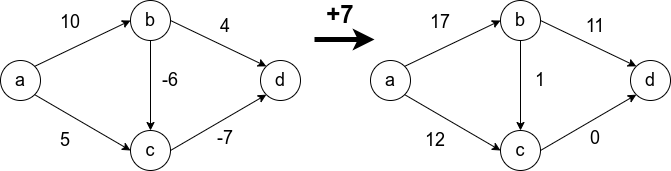
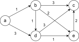
Условие неотрицательности весов рёбер крайне важно и от него нельзя просто избавиться. Не получится свести задачу к решаемой алгоритмом Дейкстры, прибавив наибольший по модулю вес ко всем рёбрам. Это может изменить оптимальный маршрут. На рисунке видно, что в первом случае оптимальный путь между  и
и  (сумма рёбер на пути наименьшая) изменяется при такой манипуляции. В оригинале путь проходит через
  , а после добавления семёрки ко всем рёбрам, оптимальный путь проходит через
Как ведёт себя алгоритм Дейкстры на исходном графе, мы разберём, когда выпишем алгоритм. Но для начала зададимся другим вопросом: «почему не применить поиск в ширину для нашего графа?». Известно, что метод BFS находит оптимальный путь от произвольной вершины в ориентированном графе до любой другой вершины, но это справедливо только для рёбер с единичным весом.
Свести задачу к решаемой BFS можно, но если заменить все рёбра неединичной длины  рёбрами длины
  , то граф очень разрастётся, и это приведёт к огромному числу действий при вычислении оптимального маршрута.
Чтобы этого избежать предлагается использовать алгоритм Дейкстры. Опишем его:
Инициализация:
Основный цикл алгоритма:
- Пока все вершины не исследованы (или формально
 ), повторяем:
 ), повторяем:
В итоге исполнения этого алгоритма, массив  будет содержать все оптимальные пути, исходящие из .
Примеры работы
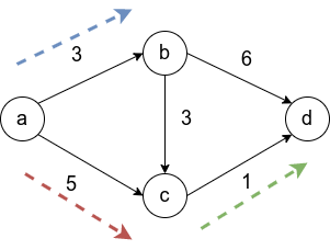
Рассмотрим граф выше, в нём будем искать пути от до всего остального.
Первый шаг алгоритма определит, что кратчайший путь до  проходит по направлению синей стрелки и зафиксирует кратчайший путь. Второй шаг рассмотрит, все возможные варианты
 ![inline A[v] + l_{vw}](https://habrastorage.org/getpro/habr/post_images/c10/6ca/2df/c106ca2df0651dd2d791b59d6959e8fb.svg) и окажется, что оптимальный вариант двигаться вдоль красной стрелки, поскольку
и окажется, что оптимальный вариант двигаться вдоль красной стрелки, поскольку  меньше, чем
  и
и  Добавляется длина кратчайшего пути до
  . И наконец, третьим шагом, когда три вершины
  уже лежат в
  , остается рассмотреть только два ребра и выбрать, лежащее вдоль зеленой стрелки.
Теперь рассмотрим граф с отрицательными весами, упомянутый выше. Напомню, алгоритм Дейкстры на таком графе может работать некорректно.
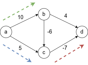
Первым шагом отбирается ребро вдоль синей стрелки, поскольку это ребро наименьшего веса из исходной вершины. Затем выбирается ребро  Это зафиксирует навсегда неверный путь от к , в то время как оптимальный путь проходит через центр с отрицательным весом. Последним шагом, будет добавлена вершина .
Оценка сложности алгоритма
К этому моменту мы разобрали сам алгоритм, ограничения, накладываемые на его работу и ряд примеров его применения. Давайте упомянем какова вычислительная сложность этого алгоритма, поскольку это пригодится нам для решения задач, ради которых затевалась эта статья.
Базовый подход, основанный на циклах, предполагает проход по всем рёбрам каждого узла, что приводит к сложности  .
.
Эффективная реализация предполагает использование кучи. Об этой структуре данных можно сказать коротко: она позволяет выполнять две операции за логарифмическое время. Первая операция — получение узла в дереве, с наименьшим ключом, и, вторая операция, вставка нового узла в дерево с новым ключом.
Что еще можно сказать о куче:
- это сбалансированное бинарное дерево,
- ключ текущего узла всегда меньше, либо равен ключей дочерних узлов.
Интересную задачу с использованием куч я разбирал ранее в этом посте.
Используя кучу в алгоритме Дейкстры, где в качестве ключей используются расстояния от вершины в неисследованной части графа (в алгоритме это  ), до ближайшей вершины в уже покрытом (это множество вершин ), можно сократить вычислительную сложность до
  Доказательство справедливости этих оценок я оставляю за пределами этой статьи.
Далее перейдём к разбору задач!
Задача №1
Будем называть узким местом пути в графе ребро максимальной длины в этом пути. Путём с минимальным узким местом назовём такой путь между вершинами и , что не существует другого пути  , чьё узкое место меньше по длине. Требуется построить алгоритм, который вычисляет путь с минимальным узким местом для двух данных вершин в графе. Асимптотическая сложность такого алгоритма должна быть
Решение
По условию задачи ребро с большим весом трактуется как узкое место. Вес в этом случае можно воспринимать как цену за проход по ребру. В результате решения задачи хотелось бы получить алгоритм, способный строить маршруты между узлами так, чтобы, если мы захотим провести любой другой путь, он будет содержать более тяжелые рёбра.
В случае классической задачи, поиска пути минимальной длины между двумя вершинами графа, мы поддерживаем в каждой посещенной алгоритмом вершине графа минимальную длину пути до этой вершины. Здесь стоит оговориться, что будем именовать множество посещенными вершинами, а часть графа, для которой еще нужно найти величину пути или узкого места.
В отличии от классического алгоритма, решение этой задачи должно поддерживать величину актуального узкого места пути, приводящего в вершину  . А при добавлении новой вершины из , мы должны смотреть не увеличивает ли ребро
  величину узкого места пути, которое теперь приводит в
  .
.
Если ребро увеличивает узкое место, то лучше рассмотреть вершину  , ребро
  до которой легче . Поиск неувеличивающих узкое место ребёр нужно осуществлять не только среди соседей определенного узла
  , но и среди всех , поскольку отдавая предпочтение вершине, путь в которую имеет наименьшее узкое место в данный момент, мы гарантируем, что мы не ухудшаем ситуацию для других вершин.
Последнее можно проиллюстрировать примером: если путь, оканчивающийся в вершине  имеет узкое место величины
  , и есть вершина
  с ребром
  веса
веса  , и
, и  с ребром
  веса , то предпочтение отдаётся , алгоритм даст верный результат в обоих случая, если существует
  веса или веса
  .
.
В результате разбора выше, предлагается руководствоваться следующей формулой при выборе очередной вершины из непосещенных и обновлении величин, которые мы поддерживаем.
![A(u) = min_{v in X}left(max left[A(v), wleft(v,uright)right]right), , u in V - X](https://habrastorage.org/getpro/habr/post_images/6bf/459/cbd/6bf459cbdc59a4ffaf8b7bfe68ed0f27.svg)
Стоит пояснить, что поиск по осуществляется, только для существующих связей  а
а  это вес ребра
  .
.
Задача №2
Предлагается решить более практическую задачу. Пусть городов, между ними существуют пути, заданные массивом edges[i] = [city_a, city_b, distance_ab], а также дано целое число mileage.
Требуется найти такой город из данных, из которого можно добраться до наименьшего числа городов не превысив mileage.
Стоит отметить, что граф неориентированый, т.е. по пути между городами можно двигаться в обе стороны, а длина пути между городами a и c может быть получена как сумма длин путей a -> b и b -> c, если есть маршрут a -> b -> c
Решение
С решением данной проблемы нам поможет алгоритм Дейкстры и описанная выше реализация с помощью кучи. Поставщиком этой структуры данных станет библиотека heapq в Python.
Будем использовать алгоритм Дейкстры для того, чтобы подсчитать количество соседних городов, расстояние до которых меньше mileage, для каждого из городов. Соберем количества соседей в в одном месте и найдем минимум из них.
Поскольку наш граф неориентированный, то из любой его вершины можно добраться до произвольной вершины . Будем использовать алгоритм Дейкстры для того, чтобы для каждого из городов в графе построить кратчайшие пути до всех остальных городов, мы это уже умеем делать в теории. И чтобы, оптимизировать этот процесс, будем в его течении сразу отвергать пути, которые превышают mileage, а не делать постфактум, когда все пути получены.
Давайте опишем функцию решения:
def least_reachable_city(n, edges, mileage):
        """
        входные параметры:
            n --- количество городов,
            edges --- тройки (a, b, distance_ab),
            mileage --- максимально допустимое расстояние между городами
            для соседства
        """
        # заполняем список смежности (adjacency list), в нашем случае это
        # словарь, в котором ключи это города, а значения --- пары
        # (<другой_город>, <расстояние_до_него>)

        graph = {}
        for u, v, w in edges:
            if graph.get(u, None) is None:
                graph[u] = [(v, w)]
            else:
                graph[u].append((v, w))
            if graph.get(v, None) is None:
                graph[v] = [(u, w)]
            else:
                graph[v].append((u, w))

        # локально объявим функцию, которая будет считать кратчайшие пути в
        # графе от вершины, до всех вершин, удовлетворяющих условию
        def num_reachable_neighbors(city):
            # создаем кучу, из одного элемента с парой, задающей нулевую
            # длину пути до самого исходного города
            heap = [(0, city)]
            # и массив, содержащий города и кратчайшие
            # расстояния до них от исходного
            distances = {}
            # затем, пока куча не пуста, извлекаем ближайший
            # от посещенных городов город
            while heap:
                currDist, neighb = heapq.heappop(heap)
                # если кратчайшее ребро ведет к городу, где мы уже знаем
                # оптимальный маршрут, то завершаем итерацию
                if neighb in distances:
                    continue
                # в остальных случаях, и если сосед не является отправным
                # городом, мы добавляем новую запись в массив кратчайших расстояний
                if neighb != city:
                    distances[neighb] = currDist
                # обрабатываем всех смежных городов с соседом, добавляя их в кучу
                # но только если: а) до них еще не известен кратчайший маршрут и б) путь до них через neighb не выходит за пределы mileage
                for node, d in graph[neighb]:
                    if node in distances:
                        continue
                    if currDist + d <= mileage:
                        heapq.heappush(heap, (currDist + d, node))
            # возвращаем количество городов, прошедших проверку
            return len(distances)

        # выполним поиск соседей для каждого из городов
        cities_neighbors = {num_reachable_neighbors(city): city for city in range(n)}
        # вернём номер города, у которого наименьшее число соседей
        # в пределах досигаемости
        return cities_neighbors[min(cities_neighbors)]
В функции выше, в комментариях, подробно описывается, как метод Дейкстры, реализованный на куче позволяет найти расстояния до всех городов, в пределах `mileage`. Основную сложность для понимания предстваляет цикл, работающий с кучей.
Заключение
Алгоритм Дейкстры это мощный инструмент в мире работы с графами, область применения его крайне широка. С его помощью можно оценить даже целесообразность добавления новой ветки метро, новой дороги или маршрута в компьютерной сети. Он прост в исполнении и интуитивно понятен, как другие жадные (greedy) алгоритмы. Вычислительная сложность решений задач с его помощью зачастую не выше  . При некоторых условиях может достигать линейной сложности (существует алгоритм линейной сложности, решающий первую задачу, при условии, что граф неориентированный).
Стоит еще раз отметить, что алгоритм не работает, когда в графе существуют отрицательные веса. Для этого существует подход динамического программирования — алгоритм Беллмана – Форда, что может послужить темой другой статьи. Несмотря на это, алгоритм Дейкстры является представителем идеального баланса простоты и мощи, для решения прикладных задач.
Статья подготовлена в преддверии старта курса «Алгоритмы для разработчиков». Узнать о курсе подробнее, а также зарегистрироваться на бесплатный демоурок можно по ссылке.
Информация
[1] Условия задач взяты из книги «Algorithms Illuminated: Part 2: Graph Algorithms and Data Structures» от Tim Roughgarden,
[2] и с сайта leetcode.com.
[3] Решения авторские.
Графы. Нахождение кратчайшего расстояния между двумя вершинами с помощью алгоритма Дейкстры
- Подробности
- Категория: Сортировка и поиск
Алгоритм Дейкстры (англ. Dijkstra’s algorithm) — алгоритм на графах, изобретённый нидерландским учёным Эдсгером Дейкстрой в 1959 году. Находит кратчайшие пути от одной из вершин графа до всех остальных. Алгоритм работает только для графов без рёбер отрицательного веса.

Лекция 2: Алгоритмы и методы сортировки. Алгоритмы нахождения кратчайшего пути в графе
Лекция 5: Поиск в графах и обход. Алгоритм Дейкстры
Алгоритмы и структуры данных, лекция 13
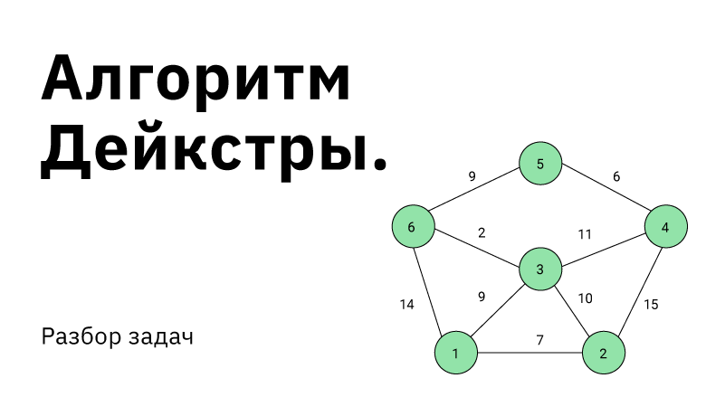
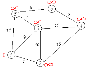
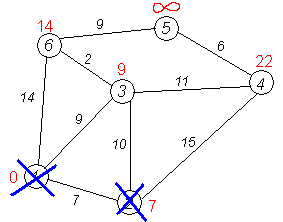
Рассмотрим выполнение алгоритма на примере графа, показанного на рисунке.
Пусть требуется найти кратчайшие расстояния от 1-й вершины до всех остальных.

Кружками обозначены вершины, линиями — пути между ними (рёбра графа). В кружках обозначены номера вершин, над рёбрами обозначена их «цена» — длина пути. Рядом с каждой вершиной красным обозначена метка — длина кратчайшего пути в эту вершину из вершины 1.
Первый шаг. Рассмотрим шаг алгоритма Дейкстры для нашего примера. Минимальную метку имеет вершина 1. Её соседями являются вершины 2, 3 и 6.

Первый по очереди сосед вершины 1 — вершина 2, потому что длина пути до неё минимальна. Длина пути в неё через вершину 1 равна сумме значения метки вершины 1 и длины ребра, идущего из 1-й в 2-ю, то есть 0 + 7 = 7. Это меньше текущей метки вершины 2, бесконечности, поэтому новая метка 2-й вершины равна 7.
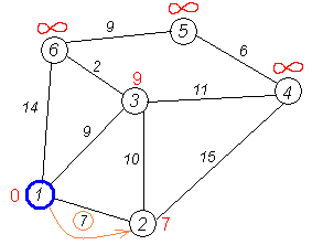
Аналогичную операцию проделываем с двумя другими соседями 1-й вершины — 3-й и 6-й.

Все соседи вершины 1 проверены. Текущее минимальное расстояние до вершины 1 считается окончательным и пересмотру не подлежит (то, что это действительно так, впервые доказал Э. Дейкстра). Вычеркнем её из графа, чтобы отметить, что эта вершина посещена.

Второй шаг. Шаг алгоритма повторяется. Снова находим «ближайшую» из непосещённых вершин. Это вершина 2 с меткой 7.
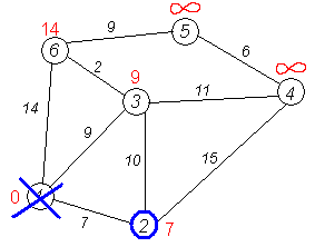
Снова пытаемся уменьшить метки соседей выбранной вершины, пытаясь пройти в них через 2-ю вершину. Соседями вершины 2 являются вершины 1, 3 и 4.
Первый (по порядку) сосед вершины 2 — вершина 1. Но она уже посещена, поэтому с 1-й вершиной ничего не делаем.
Следующий сосед вершины 2 — вершина 3, так как имеет минимальную метку из вершин, отмеченных как не посещённые. Если идти в неё через 2, то длина такого пути будет равна 17 (7 + 10 = 17). Но текущая метка третьей вершины равна 9, а это меньше 17, поэтому метка не меняется.

Ещё один сосед вершины 2 — вершина 4. Если идти в неё через 2-ю, то длина такого пути будет равна сумме кратчайшего расстояния до 2-й вершины и расстояния между вершинами 2 и 4, то есть 22 (7 + 15 = 22). Поскольку 22< , устанавливаем метку вершины 4 равной 22.

Все соседи вершины 2 просмотрены, замораживаем расстояние до неё и помечаем её как посещённую.
Третий шаг. Повторяем шаг алгоритма, выбрав вершину 3. После её «обработки» получим такие результаты:

Дальнейшие шаги. Повторяем шаг алгоритма для оставшихся вершин. Это будут вершины 6, 4 и 5, соответственно порядку.

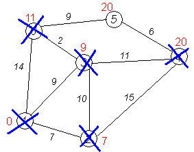

Завершение выполнения алгоритма. Алгоритм заканчивает работу, когда нельзя больше обработать ни одной вершины. В данном примере все вершины зачёркнуты, однако ошибочно полагать, что так будет в любом примере — некоторые вершины могут остаться незачёркнутыми, если до них нельзя добраться, т. е. если граф несвязный. Результат работы алгоритма виден на последнем рисунке: кратчайший путь от вершины 1 до 2-й составляет 7, до 3-й — 9, до 4-й — 20, до 5-й — 20, до 6-й — 11.
Реализация алгоритма на различных языках программирования :
C++
#include "stdafx.h"
#include <iostream>
using namespace std;
const int V=6;
//алгоритм Дейкстры
void Dijkstra(int GR[V][V], int st)
{
int distance[V], count, index, i, u, m=st+1;
bool visited[V];
for (i=0; i<V; i++)
{
distance[i]=INT_MAX; visited[i]=false;
}
distance[st]=0;
for (count=0; count<V-1; count++)
{
int min=INT_MAX;
for (i=0; i<V; i++)
if (!visited[i] && distance[i]<=min)
{
min=distance[i]; index=i;
}
u=index;
visited[u]=true;
for (i=0; i<V; i++)
if (!visited[i] && GR[u][i] && distance[u]!=INT_MAX &&
distance[u]+GR[u][i]<distance[i])
distance[i]=distance[u]+GR[u][i];
}
cout<<"Стоимость пути из начальной вершины до остальных:tn";
for (i=0; i<V; i++) if (distance[i]!=INT_MAX)
cout<<m<<" > "<<i+1<<" = "<<distance[i]<<endl;
else cout<<m<<" > "<<i+1<<" = "<<"маршрут недоступен"<<endl;
}
//главная функция
void main()
{
setlocale(LC_ALL, "Rus");
int start, GR[V][V]={
{0, 1, 4, 0, 2, 0},
{0, 0, 0, 9, 0, 0},
{4, 0, 0, 7, 0, 0},
{0, 9, 7, 0, 0, 2},
{0, 0, 0, 0, 0, 8},
{0, 0, 0, 0, 0, 0}};
cout<<"Начальная вершина >> "; cin>>start;
Dijkstra(GR, start-1);
system("pause>>void");
}
kvodo
Pascal
program DijkstraAlgorithm;
uses crt;
const V=6; inf=100000;
type vektor=array[1..V] of integer;
var start: integer;
const GR: array[1..V, 1..V] of integer=(
(0, 1, 4, 0, 2, 0),
(0, 0, 0, 9, 0, 0),
(4, 0, 0, 7, 0, 0),
(0, 9, 7, 0, 0, 2),
(0, 0, 0, 0, 0, 8),
(0, 0, 0, 0, 0, 0));
{алгоритм Дейкстры}
procedure Dijkstra(GR: array[1..V, 1..V] of integer; st: integer);
var count, index, i, u, m, min: integer;
distance: vektor;
visited: array[1..V] of boolean;
begin
m:=st;
for i:=1 to V do
begin
distance[i]:=inf; visited[i]:=false;
end;
distance[st]:=0;
for count:=1 to V-1 do
begin
min:=inf;
for i:=1 to V do
if (not visited[i]) and (distance[i]<=min) then
begin
min:=distance[i]; index:=i;
end;
u:=index;
visited[u]:=true;
for i:=1 to V do
if (not visited[i]) and (GR[u, i]<>0) and (distance[u]<>inf) and
(distance[u]+GR[u, i]<distance[i]) then
distance[i]:=distance[u]+GR[u, i];
end;
write('Стоимость пути из начальной вершины до остальных:'); writeln;
for i:=1 to V do
if distance[i]<>inf then
writeln(m,' > ', i,' = ', distance[i])
else writeln(m,' > ', i,' = ', 'маршрут недоступен');
end;
{основной блок программы}
begin
clrscr;
write('Начальная вершина >> '); read(start);
Dijkstra(GR, start);
end.
kvodo
Java
import java.io.BufferedReader;
import java.io.IOException;
import java.io.InputStreamReader;
import java.io.PrintWriter;
import java.util.ArrayList;
import java.util.Arrays;
import java.util.StringTokenizer;

public class Solution {

    private static int INF = Integer.MAX_VALUE / 2;

    private int n; //количество вершин в орграфе
    private int m; //количествое дуг в орграфе
    private ArrayList<Integer> adj[]; //список смежности
    private ArrayList<Integer> weight[]; //вес ребра в орграфе
    private boolean used[]; //массив для хранения информации о пройденных и не пройденных вершинах
    private int dist[]; //массив для хранения расстояния от стартовой вершины
    //массив предков, необходимых для восстановления кратчайшего пути из стартовой вершины
    private int pred[];
    int start; //стартовая вершина, от которой ищется расстояние до всех других

    private BufferedReader cin;
    private PrintWriter cout;
    private StringTokenizer tokenizer;

    //процедура запуска алгоритма Дейкстры из стартовой вершины
    private void dejkstra(int s) {
        dist[s] = 0; //кратчайшее расстояние до стартовой вершины равно 0
        for (int iter = 0; iter < n; ++iter) {
            int v = -1;
            int distV = INF;
            //выбираем вершину, кратчайшее расстояние до которого еще не найдено
            for (int i = 0; i < n; ++i) {
                if (used[i]) {
                    continue;
                }
                if (distV < dist[i]) {
                    continue;
                }
                v = i;
                distV = dist[i];
            }
            //рассматриваем все дуги, исходящие из найденной вершины
            for (int i = 0; i < adj[v].size(); ++i) {
                int u = adj[v].get(i);
                int weightU = weight[v].get(i);
                //релаксация вершины
                if (dist[v] + weightU < dist[u]) {
                    dist[u] = dist[v] + weightU;
                    pred[u] = v;
                }
            }
            //помечаем вершину v просмотренной, до нее найдено кратчайшее расстояние
            used[v] = true;
        }
    }

    //процедура считывания входных данных с консоли
    private void readData() throws IOException {
        cin = new BufferedReader(new InputStreamReader(System.in));
        cout = new PrintWriter(System.out);
        tokenizer = new StringTokenizer(cin.readLine());

        n = Integer.parseInt(tokenizer.nextToken()); //считываем количество вершин графа
        m = Integer.parseInt(tokenizer.nextToken()); //считываем количество ребер графа
        start = Integer.parseInt(tokenizer.nextToken()) - 1;

        //инициализируем списка смежности графа размерности n
        adj = new ArrayList[n];
        for (int i = 0; i < n; ++i) {
            adj[i] = new ArrayList<Integer>();
        }
        //инициализация списка, в котором хранятся веса ребер
        weight = new ArrayList[n];
        for (int i = 0; i < n; ++i) {
            weight[i] = new ArrayList<Integer>();
        }

        //считываем граф, заданный списком ребер
        for (int i = 0; i < m; ++i) {
            tokenizer = new StringTokenizer(cin.readLine());
            int u = Integer.parseInt(tokenizer.nextToken());
            int v = Integer.parseInt(tokenizer.nextToken());
            int w = Integer.parseInt(tokenizer.nextToken());
            u--;
            v--;
            adj[u].add(v);
            weight[u].add(w);
        }

        used = new boolean[n];
        Arrays.fill(used, false);

        pred = new int[n];
        Arrays.fill(pred, -1);

        dist = new int[n];
        Arrays.fill(dist, INF);

    }

    //процедура восстановления кратчайшего пути по массиву предком
    void printWay(int v) {
        if (v == -1) {
            return;
        }
        printWay(pred[v]);
        cout.print((v + 1) + " ");
    }

    //процедура вывода данных в консоль
    private void printData() throws IOException {
        for (int v = 0; v < n; ++v) {
            if (dist[v] != INF) {
                cout.print(dist[v] + " ");
            } else {
                cout.print("-1 ");
            }
        }
        cout.println();
        for (int v = 0; v < n; ++v) {
            cout.print((v + 1) + ": ");
            if (dist[v] != INF) {
                printWay(v);
            }
            cout.println();
        }

        cin.close();
        cout.close();
    }

    private void run() throws IOException {
        readData();
        dejkstra(start);
        printData();

        cin.close();
        cout.close();
    }

    public static void main(String[] args) throws IOException {
        Solution solution = new Solution();
        solution.run();
    }
}
cybern.ru
Ещё один вариант:
import java.io.*;
import java.util.*;

public class Dijkstra {
   private static final Graph.Edge[] GRAPH = {
      new Graph.Edge("a", "b", 7),
      new Graph.Edge("a", "c", 9),
      new Graph.Edge("a", "f", 14),
      new Graph.Edge("b", "c", 10),
      new Graph.Edge("b", "d", 15),
      new Graph.Edge("c", "d", 11),
      new Graph.Edge("c", "f", 2),
      new Graph.Edge("d", "e", 6),
      new Graph.Edge("e", "f", 9),
   };
   private static final String START = "a";
   private static final String END = "e";

   public static void main(String[] args) {
      Graph g = new Graph(GRAPH);
      g.dijkstra(START);
      g.printPath(END);
      //g.printAllPaths();
   }
}

class Graph {
   private final Map<String, Vertex> graph; // mapping of vertex names to Vertex objects, built from a set of Edges

   /** One edge of the graph (only used by Graph constructor) */
   public static class Edge {
      public final String v1, v2;
      public final int dist;
      public Edge(String v1, String v2, int dist) {
         this.v1 = v1;
         this.v2 = v2;
         this.dist = dist;
      }
   }

   /** One vertex of the graph, complete with mappings to neighbouring vertices */
   public static class Vertex implements Comparable<Vertex> {
      public final String name;
      public int dist = Integer.MAX_VALUE; // MAX_VALUE assumed to be infinity
      public Vertex previous = null;
      public final Map<Vertex, Integer> neighbours = new HashMap<>();

      public Vertex(String name) {
         this.name = name;
      }

      private void printPath() {
         if (this == this.previous) {
            System.out.printf("%s", this.name);
         } else if (this.previous == null) {
            System.out.printf("%s(unreached)", this.name);
         } else {
            this.previous.printPath();
            System.out.printf(" -> %s(%d)", this.name, this.dist);
         }
      }

      public int compareTo(Vertex other) {
         return Integer.compare(dist, other.dist);
      }
   }

   /** Builds a graph from a set of edges */
   public Graph(Edge[] edges) {
      graph = new HashMap<>(edges.length);

      //one pass to find all vertices
      for (Edge e : edges) {
         if (!graph.containsKey(e.v1)) graph.put(e.v1, new Vertex(e.v1));
         if (!graph.containsKey(e.v2)) graph.put(e.v2, new Vertex(e.v2));
      }

      //another pass to set neighbouring vertices
      for (Edge e : edges) {
         graph.get(e.v1).neighbours.put(graph.get(e.v2), e.dist);
         //graph.get(e.v2).neighbours.put(graph.get(e.v1), e.dist); // also do this for an undirected graph
      }
   }

   /** Runs dijkstra using a specified source vertex */
   public void dijkstra(String startName) {
      if (!graph.containsKey(startName)) {
         System.err.printf("Graph doesn't contain start vertex "%s"n", startName);
         return;
      }
      final Vertex source = graph.get(startName);
      NavigableSet<Vertex> q = new TreeSet<>();

      // set-up vertices
      for (Vertex v : graph.values()) {
         v.previous = v == source ? source : null;
         v.dist = v == source ? 0 : Integer.MAX_VALUE;
         q.add(v);
      }

      dijkstra(q);
   }

   /** Implementation of dijkstra's algorithm using a binary heap. */
   private void dijkstra(final NavigableSet<Vertex> q) {
      Vertex u, v;
      while (!q.isEmpty()) {

         u = q.pollFirst(); // vertex with shortest distance (first iteration will return source)
         if (u.dist == Integer.MAX_VALUE) break; // we can ignore u (and any other remaining vertices) since they are unreachable

         //look at distances to each neighbour
         for (Map.Entry<Vertex, Integer> a : u.neighbours.entrySet()) {
            v = a.getKey(); //the neighbour in this iteration

            final int alternateDist = u.dist + a.getValue();
            if (alternateDist < v.dist) { // shorter path to neighbour found
               q.remove(v);
               v.dist = alternateDist;
               v.previous = u;
               q.add(v);
            }
         }
      }
   }

   /** Prints a path from the source to the specified vertex */
   public void printPath(String endName) {
      if (!graph.containsKey(endName)) {
         System.err.printf("Graph doesn't contain end vertex "%s"n", endName);
         return;
      }

      graph.get(endName).printPath();
      System.out.println();
   }
   /** Prints the path from the source to every vertex (output order is not guaranteed) */
   public void printAllPaths() {
      for (Vertex v : graph.values()) {
         v.printPath();
         System.out.println();
      }
   }
}
rosettacode.org
C
#include <stdio.h>
#include <stdlib.h>
#include <string.h>

//#define BIG_EXAMPLE

typedef struct node_t node_t, *heap_t;
typedef struct edge_t edge_t;
struct edge_t {
	node_t *nd;	/* target of this edge */
	edge_t *sibling;/* for singly linked list */
	int len;	/* edge cost */
};
struct node_t {
	edge_t *edge;	/* singly linked list of edges */
	node_t *via;	/* where previous node is in shortest path */
	double dist;	/* distance from origining node */
	char name[8];	/* the, er, name */
	int heap_idx;	/* link to heap position for updating distance */
};


/* --- edge management --- */
#ifdef BIG_EXAMPLE
#	define BLOCK_SIZE (1024 * 32 - 1)
#else
#	define BLOCK_SIZE 15
#endif
edge_t *edge_root = 0, *e_next = 0;

/* Don't mind the memory management stuff, they are besides the point.
   Pretend e_next = malloc(sizeof(edge_t)) */
void add_edge(node_t *a, node_t *b, double d)
{
	if (e_next == edge_root) {
		edge_root = malloc(sizeof(edge_t) * (BLOCK_SIZE + 1));
		edge_root[BLOCK_SIZE].sibling = e_next;
		e_next = edge_root + BLOCK_SIZE;
	}
	--e_next;

	e_next->nd = b;
	e_next->len = d;
	e_next->sibling = a->edge;
	a->edge = e_next;
}

void free_edges()
{
	for (; edge_root; edge_root = e_next) {
		e_next = edge_root[BLOCK_SIZE].sibling;
		free(edge_root);
	}
}

/* --- priority queue stuff --- */
heap_t *heap;
int heap_len;

void set_dist(node_t *nd, node_t *via, double d)
{
	int i, j;

	/* already knew better path */
	if (nd->via && d >= nd->dist) return;

	/* find existing heap entry, or create a new one */
	nd->dist = d;
	nd->via = via;

	i = nd->heap_idx;
	if (!i) i = ++heap_len;

	/* upheap */
	for (; i > 1 && nd->dist < heap[j = i/2]->dist; i = j)
		(heap[i] = heap[j])->heap_idx = i;

	heap[i] = nd;
	nd->heap_idx = i;
}

node_t * pop_queue()
{
	node_t *nd, *tmp;
	int i, j;

	if (!heap_len) return 0;

	/* remove leading element, pull tail element there and downheap */
	nd = heap[1];
	tmp = heap[heap_len--];

	for (i = 1; i < heap_len && (j = i * 2) <= heap_len; i = j) {
		if (j < heap_len && heap[j]->dist > heap[j+1]->dist) j++;

		if (heap[j]->dist >= tmp->dist) break;
		(heap[i] = heap[j])->heap_idx = i;
	}

	heap[i] = tmp;
	tmp->heap_idx = i;

	return nd;
}

/* --- Dijkstra stuff; unreachable nodes will never make into the queue --- */
void calc_all(node_t *start)
{
	node_t *lead;
	edge_t *e;

	set_dist(start, start, 0);
	while ((lead = pop_queue()))
		for (e = lead->edge; e; e = e->sibling)
			set_dist(e->nd, lead, lead->dist + e->len);
}

void show_path(node_t *nd)
{
	if (nd->via == nd)
		printf("%s", nd->name);
	else if (!nd->via)
		printf("%s(unreached)", nd->name);
	else {
		show_path(nd->via);
		printf("-> %s(%g) ", nd->name, nd->dist);
	}
}

int main(void)
{
#ifndef BIG_EXAMPLE
	int i;

#	define N_NODES ('f' - 'a' + 1)
	node_t *nodes = calloc(sizeof(node_t), N_NODES);

	for (i = 0; i < N_NODES; i++)
		sprintf(nodes[i].name, "%c", 'a' + i);

#	define E(a, b, c) add_edge(nodes + (a - 'a'), nodes + (b - 'a'), c)
	E('a', 'b', 7);	E('a', 'c', 9); E('a', 'f', 14);
	E('b', 'c', 10);E('b', 'd', 15);E('c', 'd', 11);
	E('c', 'f', 2); E('d', 'e', 6);	E('e', 'f', 9);
#	undef E

#else /* BIG_EXAMPLE */
	int i, j, c;

#	define N_NODES 4000
	node_t *nodes = calloc(sizeof(node_t), N_NODES);

	for (i = 0; i < N_NODES; i++)
		sprintf(nodes[i].name, "%d", i + 1);

	/* given any pair of nodes, there's about 50% chance they are not
	   connected; if connected, the cost is randomly chosen between 0
	   and 49 (inclusive! see output for consequences) */
	for (i = 0; i < N_NODES; i++) {
		for (j = 0; j < N_NODES; j++) {
			/* majority of runtime is actually spent here */
			if (i == j) continue;
			c = rand() % 100;
			if (c < 50) continue;
			add_edge(nodes + i, nodes + j, c - 50);
		}
	}

#endif
	heap = calloc(sizeof(heap_t), N_NODES + 1);
	heap_len = 0;

	calc_all(nodes);
	for (i = 0; i < N_NODES; i++) {
		show_path(nodes + i);
		putchar('n');
	}

#if 0
	/* real programmers don't free memories (they use Fortran) */
	free_edges();
	free(heap);
	free(nodes);
#endif
	return 0;
}
rosettacode.org
PHP
<?php
function dijkstra($graph_array, $source, $target) {
    $vertices = array();
    $neighbours = array();
    foreach ($graph_array as $edge) {
        array_push($vertices, $edge[0], $edge[1]);
        $neighbours[$edge[0]][] = array("end" => $edge[1], "cost" => $edge[2]);
        $neighbours[$edge[1]][] = array("end" => $edge[0], "cost" => $edge[2]);
    }
    $vertices = array_unique($vertices);

    foreach ($vertices as $vertex) {
        $dist[$vertex] = INF;
        $previous[$vertex] = NULL;
    }

    $dist[$source] = 0;
    $Q = $vertices;
    while (count($Q) > 0) {

        // TODO - Find faster way to get minimum
        $min = INF;
        foreach ($Q as $vertex){
            if ($dist[$vertex] < $min) {
                $min = $dist[$vertex];
                $u = $vertex;
            }
        }

        $Q = array_diff($Q, array($u));
        if ($dist[$u] == INF or $u == $target) {
            break;
        }

        if (isset($neighbours[$u])) {
            foreach ($neighbours[$u] as $arr) {
                $alt = $dist[$u] + $arr["cost"];
                if ($alt < $dist[$arr["end"]]) {
                    $dist[$arr["end"]] = $alt;
                    $previous[$arr["end"]] = $u;
                }
            }
        }
    }
    $path = array();
    $u = $target;
    while (isset($previous[$u])) {
        array_unshift($path, $u);
        $u = $previous[$u];
    }
    array_unshift($path, $u);
    return $path;
}

$graph_array = array(
                    array("a", "b", 7),
                    array("a", "c", 9),
                    array("a", "f", 14),
                    array("b", "c", 10),
                    array("b", "d", 15),
                    array("c", "d", 11),
                    array("c", "f", 2),
                    array("d", "e", 6),
                    array("e", "f", 9)
               );

$path = dijkstra($graph_array, "a", "e");

echo "path is: ".implode(", ", $path)."n";
Output is:
path is: a, c, f, e
rosettacode.org
Python
from collections import namedtuple, queue
from pprint import pprint as pp


inf = float('inf')
Edge = namedtuple('Edge', 'start, end, cost')

class Graph():
    def __init__(self, edges):
        self.edges = edges2 = [Edge(*edge) for edge in edges]
        self.vertices = set(sum(([e.start, e.end] for e in edges2), []))

    def dijkstra(self, source, dest):
        assert source in self.vertices
        dist = {vertex: inf for vertex in self.vertices}
        previous = {vertex: None for vertex in self.vertices}
        dist[source] = 0
        q = self.vertices.copy()
        neighbours = {vertex: set() for vertex in self.vertices}
        for start, end, cost in self.edges:
            neighbours[start].add((end, cost))
        #pp(neighbours)

        while q:
            u = min(q, key=lambda vertex: dist[vertex])
            q.remove(u)
            if dist[u] == inf or u == dest:
                break
            for v, cost in neighbours[u]:
                alt = dist[u] + cost
                if alt < dist[v]:                                  # Relax (u,v,a)
                    dist[v] = alt
                    previous[v] = u
        #pp(previous)
        s, u = deque(), dest
        while previous[u]:
            s.pushleft(u)
            u = previous[u]
        s.pushleft(u)
        return s


graph = Graph([("a", "b", 7),  ("a", "c", 9),  ("a", "f", 14), ("b", "c", 10),
               ("b", "d", 15), ("c", "d", 11), ("c", "f", 2),  ("d", "e", 6),
               ("e", "f", 9)])
pp(graph.dijkstra("a", "e"))

Output:

['a', 'c', 'd', 'e']
rosettacode.org
Рассмотрим пример нахождение кратчайшего пути. Дана сеть автомобильных дорог, соединяющих области города. Некоторые дороги односторонние. Найти кратчайшие пути от центра города до каждого города области.
Для решения указанной задачи можно использовать алгоритм Дейкстры — алгоритм на графах, изобретённый нидерландским ученым Э. Дейкстрой в 1959 году. Находит кратчайшее расстояние от одной из вершин графа до всех остальных. Работает только для графов без рёбер отрицательного веса.
Пусть требуется найти кратчайшие расстояния от 1-й вершины до всех остальных.
Кружками обозначены вершины, линиями – пути между ними (ребра графа). В кружках обозначены номера вершин, над ребрами обозначен их вес – длина пути. Рядом с каждой вершиной красным обозначена метка – длина кратчайшего пути в эту вершину из вершины 1.

Инициализация
Метка самой вершины 1 полагается равной 0, метки остальных вершин – недостижимо большое число (в идеале — бесконечность). Это отражает то, что расстояния от вершины 1 до других вершин пока неизвестны. Все вершины графа помечаются как непосещенные.

Первый шаг
Минимальную метку имеет вершина 1. Её соседями являются вершины 2, 3 и 6. Обходим соседей вершины по очереди.
Первый сосед вершины 1 – вершина 2, потому что длина пути до неё минимальна. Длина пути в неё через вершину 1 равна сумме кратчайшего расстояния до вершины 1 (значению её метки) и длины ребра, идущего из 1-й во 2-ю, то есть 0 + 7 = 7. Это меньше текущей метки вершины 2 (10000), поэтому новая метка 2-й вершины равна 7.

Аналогично находим длины пути для всех других соседей (вершины 3 и 6).
Все соседи вершины 1 проверены. Текущее минимальное расстояние до вершины 1 считается окончательным и пересмотру не подлежит. Вершина 1 отмечается как посещенная.
Второй шаг
Шаг 1 алгоритма повторяется. Снова находим «ближайшую» из непосещенных вершин. Это вершина 2 с меткой 7.
Снова пытаемся уменьшить метки соседей выбранной вершины, пытаясь пройти в них через 2-ю вершину. Соседями вершины 2 являются вершины 1, 3 и 4.
Вершина 1 уже посещена. Следующий сосед вершины 2 — вершина 3, так как имеет минимальную метку из вершин, отмеченных как не посещённые. Если идти в неё через 2, то длина такого пути будет равна 17 (7 + 10 = 17). Но текущая метка третьей вершины равна 9, а 9 < 17, поэтому метка не меняется.

Ещё один сосед вершины 2 — вершина 4. Если идти в неё через 2-ю, то длина такого пути будет равна 22 (7 + 15 = 22). Поскольку 22<10000, устанавливаем метку вершины 4 равной 22.
Все соседи вершины 2 просмотрены, помечаем её как посещенную.
Третий шаг
Повторяем шаг алгоритма, выбрав вершину 3. После её «обработки» получим следующие результаты.

Четвертый шаг

Пятый шаг

Шестой шаг

Таким образом, кратчайшим путем из вершины 1 в вершину 5 будет путь через вершины 1 — 3 — 6 — 5, поскольку таким путем мы набираем минимальный вес, равный 20.
Займемся выводом кратчайшего пути. Мы знаем длину пути для каждой вершины, и теперь будем рассматривать вершины с конца. Рассматриваем конечную вершину (в данном случае — вершина 5), и для всех вершин, с которой она связана, находим длину пути, вычитая вес соответствующего ребра из длины пути конечной вершины.
Так, вершина 5 имеет длину пути 20. Она связана с вершинами 6 и 4.
Для вершины 6 получим вес 20 — 9 = 11 (совпал).
Для вершины 4 получим вес 20 — 6 = 14 (не совпал).
Если в результате мы получим значение, которое совпадает с длиной пути рассматриваемой вершины (в данном случае — вершина 6), то именно из нее был осуществлен переход в конечную вершину. Отмечаем эту вершину на искомом пути.
Далее определяем ребро, через которое мы попали в вершину 6. И так пока не дойдем до начала.
Если в результате такого обхода у нас на каком-то шаге совпадут значения для нескольких вершин, то можно взять любую из них — несколько путей будут иметь одинаковую длину.
Реализация алгоритма Дейкстры
Для хранения весов графа используется квадратная матрица. В заголовках строк и столбцов находятся вершины графа. А веса дуг графа размещаются во внутренних ячейках таблицы. Граф не содержит петель, поэтому на главной диагонали матрицы содержатся нулевые значения.
| 1 | 2 | 3 | 4 | 5 | 6 | |
| 1 | 0 | 7 | 9 | 0 | 0 | 14 |
| 2 | 7 | 0 | 10 | 15 | 0 | 0 |
| 3 | 9 | 10 | 0 | 11 | 0 | 2 |
| 4 | 0 | 15 | 11 | 0 | 6 | 0 |
| 5 | 0 | 0 | 0 | 6 | 0 | 9 |
| 6 | 14 | 0 | 2 | 0 | 9 | 0 |
Реализация на C++
1
2
3
4
5
6
7
8
9
10
11
12
13
14
15
16
17
18
19
20
21
22
23
24
25
26
27
28
29
30
31
32
33
34
35
36
37
38
39
40
41
42
43
44
45
46
47
48
49
50
51
52
53
54
55
56
57
58
59
60
61
62
63
64
65
66
67
68
69
70
71
72
73
74
75
76
77
78
79
80
81
82
83
84
85
86
87
88
89
90
91
92
93
94
95
96
97
98
99
100
101
102
103
#define _CRT_SECURE_NO_WARNINGS
#include <stdio.h>
#include <stdlib.h>
#define SIZE 6
int main()
{
int a[SIZE][SIZE]; // матрица связей
int d[SIZE]; // минимальное расстояние
int v[SIZE]; // посещенные вершины
int temp, minindex, min;
int begin_index = 0;
system(«chcp 1251»);
system(«cls»);
// Инициализация матрицы связей
for (int i = 0; i<SIZE; i++)
{
a[i][i] = 0;
for (int j = i + 1; j<SIZE; j++) {
printf(«Введите расстояние %d — %d: «, i + 1, j + 1);
scanf(«%d», &temp);
a[i][j] = temp;
a[j][i] = temp;
}
}
// Вывод матрицы связей
for (int i = 0; i<SIZE; i++)
{
for (int j = 0; j<SIZE; j++)
printf(«%5d «, a[i][j]);
printf(«n»);
}
//Инициализация вершин и расстояний
for (int i = 0; i<SIZE; i++)
{
d[i] = 10000;
v[i] = 1;
}
d[begin_index] = 0;
// Шаг алгоритма
do {
minindex = 10000;
min = 10000;
for (int i = 0; i<SIZE; i++)
{ // Если вершину ещё не обошли и вес меньше min
if ((v[i] == 1) && (d[i]<min))
{ // Переприсваиваем значения
min = d[i];
minindex = i;
}
}
// Добавляем найденный минимальный вес
// к текущему весу вершины
// и сравниваем с текущим минимальным весом вершины
if (minindex != 10000)
{
for (int i = 0; i<SIZE; i++)
{
if (a[minindex][i] > 0)
{
temp = min + a[minindex][i];
if (temp < d[i])
{
d[i] = temp;
}
}
}
v[minindex] = 0;
}
} while (minindex < 10000);
// Вывод кратчайших расстояний до вершин
printf(«nКратчайшие расстояния до вершин: n»);
for (int i = 0; i<SIZE; i++)
printf(«%5d «, d[i]);
// Восстановление пути
int ver[SIZE]; // массив посещенных вершин
int end = 4; // индекс конечной вершины = 5 — 1
ver[0] = end + 1; // начальный элемент — конечная вершина
int k = 1; // индекс предыдущей вершины
int weight = d[end]; // вес конечной вершины
while (end != begin_index) // пока не дошли до начальной вершины
{
for (int i = 0; i<SIZE; i++) // просматриваем все вершины
if (a[i][end] != 0) // если связь есть
{
int temp = weight — a[i][end]; // определяем вес пути из предыдущей вершины
if (temp == d[i]) // если вес совпал с рассчитанным
{ // значит из этой вершины и был переход
weight = temp; // сохраняем новый вес
end = i; // сохраняем предыдущую вершину
ver[k] = i + 1; // и записываем ее в массив
k++;
}
}
}
// Вывод пути (начальная вершина оказалась в конце массива из k элементов)
printf(«nВывод кратчайшего путиn»);
for (int i = k — 1; i >= 0; i—)
printf(«%3d «, ver[i]);
getchar(); getchar();
return 0;
}
Результат выполнения

Назад: Алгоритмизация
From Wikipedia, the free encyclopedia

Shortest path (A, C, E, D, F) between vertices A and F in the weighted directed graph
In graph theory, the shortest path problem is the problem of finding a path between two vertices (or nodes) in a graph such that the sum of the weights of its constituent edges is minimized.
The problem of finding the shortest path between two intersections on a road map may be modeled as a special case of the shortest path problem in graphs, where the vertices correspond to intersections and the edges correspond to road segments, each weighted by the length of the segment.
Definition[edit]
The shortest path problem can be defined for graphs whether undirected, directed, or mixed.
It is defined here for undirected graphs; for directed graphs the definition of path
requires that consecutive vertices be connected by an appropriate directed edge.
Two vertices are adjacent when they are both incident to a common edge.
A path in an undirected graph is a sequence of vertices 
such that  is adjacent to
  for
for  .
.
Such a path  is called a path of length
from  to
to  .
.
(The are variables; their numbering here relates to their position in the sequence and needs not to relate to any canonical labeling of the vertices.)
Let  be the edge incident to both and
  . Given a real-valued weight function
  , and an undirected (simple) graph
  , the shortest path from
  to
to  is the path
  (where
  and
and  ) that over all possible
  minimizes the sum
  When each edge in the graph has unit weight or
  , this is equivalent to finding the path with fewest edges.
The problem is also sometimes called the single-pair shortest path problem, to distinguish it from the following variations:
- The single-source shortest path problem, in which we have to find shortest paths from a source vertex v to all other vertices in the graph.
- The single-destination shortest path problem, in which we have to find shortest paths from all vertices in the directed graph to a single destination vertex v. This can be reduced to the single-source shortest path problem by reversing the arcs in the directed graph.
- The all-pairs shortest path problem, in which we have to find shortest paths between every pair of vertices v, v’ in the graph.
These generalizations have significantly more efficient algorithms than the simplistic approach of running a single-pair shortest path algorithm on all relevant pairs of vertices.
Algorithms[edit]
The most important algorithms for solving this problem are:
- Dijkstra’s algorithm solves the single-source shortest path problem with non-negative edge weight.
- Bellman–Ford algorithm solves the single-source problem if edge weights may be negative.
- A* search algorithm solves for single-pair shortest path using heuristics to try to speed up the search.
- Floyd–Warshall algorithm solves all pairs shortest paths.
- Johnson’s algorithm solves all pairs shortest paths, and may be faster than Floyd–Warshall on sparse graphs.
- Viterbi algorithm solves the shortest stochastic path problem with an additional probabilistic weight on each node.
Additional algorithms and associated evaluations may be found in Cherkassky, Goldberg & Radzik (1996).
Single-source shortest paths[edit]
Undirected graphs[edit]
| Weights | Time complexity | Author |
|---|---|---|
 + + |
O(V2) | Dijkstra 1959 |
| + |
O((E + V) log V) | Johnson 1977 (binary heap) |
| + |
O(E + V log V) | Fredman & Tarjan 1984 (Fibonacci heap) |
 |
O(E) | Thorup 1999 (requires constant-time multiplication) |
Unweighted graphs[edit]
| Algorithm | Time complexity | Author |
|---|---|---|
| Breadth-first search | O(E + V) |
Directed acyclic graphs (DAGs)[edit]
An algorithm using topological sorting can solve the single-source shortest path problem in time Θ(E + V) in arbitrarily-weighted DAGs.[1]
Directed graphs with nonnegative weights[edit]
The following table is taken from Schrijver (2004), with some corrections and additions.
A green background indicates an asymptotically best bound in the table; L is the maximum length (or weight) among all edges, assuming integer edge weights.
| Weights | Algorithm | Time complexity | Author |
|---|---|---|---|
|
 |
Ford 1956 | |
|
Bellman–Ford algorithm |  |
Shimbel 1955, Bellman 1958, Moore 1959 |
|
 |
Dantzig 1960 | |
|
Dijkstra’s algorithm with list |  |
Leyzorek et al. 1957, Dijkstra 1959, Minty (see Pollack & Wiebenson 1960), Whiting & Hillier 1960 |
|
Dijkstra’s algorithm with binary heap |  |
Johnson 1977 |
|
Dijkstra’s algorithm with Fibonacci heap |  |
Fredman & Tarjan 1984, Fredman & Tarjan 1987 |
|
Dial’s algorithm[2] (Dijkstra’s algorithm using a bucket queue with L buckets) |  |
Dial 1969 |
 |
Johnson 1981, Karlsson & Poblete 1983 | ||
| Gabow’s algorithm |  |
Gabow 1983, Gabow 1985 | |
 |
Ahuja et al. 1990 | ||
|
Thorup |  |
Thorup 2004 |
Directed graphs with arbitrary weights without negative cycles[edit]
| Weights | Algorithm | Time complexity | Author |
|---|---|---|---|
|
O(V 2EL) | Ford 1956 | |
|
Bellman–Ford algorithm | O(VE) | Shimbel 1955, Bellman 1958, Moore 1959 |
|
Johnson-Dijkstra with binary heap | O(V (E + log V)) | Johnson 1977 |
|
Johnson-Dijkstra with Fibonacci heap | O(V (E + log V)) | Fredman & Tarjan 1984, Fredman & Tarjan 1987, adapted after Johnson 1977 |
|
Johnson’s technique applied to Dial’s algorithm[2] | O(V (E + L)) | Dial 1969, adapted after Johnson 1977 |
Directed graphs with arbitrary weights with negative cycles[edit]
Finds a negative cycle or calculates distances to all vertices.
| Weights | Algorithm | Time complexity | Author |
|---|---|---|---|
 |
Andrew V. Goldberg |  |
Planar graphs with nonnegative weights[edit]
| Weights | Algorithm | Time complexity | Author |
|---|---|---|---|
 |
 |
Henzinger et al. 1997 |
All-pairs shortest paths[edit]
The all-pairs shortest path problem finds the shortest paths between every pair of vertices v, v’ in the graph. The all-pairs shortest paths problem for unweighted directed graphs was introduced by Shimbel (1953), who observed that it could be solved by a linear number of matrix multiplications that takes a total time of O(V4).
Undirected graph[edit]
| Weights | Time complexity | Algorithm |
|---|---|---|
| + |
O(V3) | Floyd–Warshall algorithm |
 |
 |
Seidel’s algorithm (expected running time) |
|
 |
Williams 2014 |
| + |
O(EV log α(E,V)) | Pettie & Ramachandran 2002 |
|
O(EV) | Thorup 1999 applied to every vertex (requires constant-time multiplication). |
Directed graph[edit]
| Weights | Time complexity | Algorithm |
|---|---|---|
| (no negative cycles) |
O(V3) | Floyd–Warshall algorithm |
|
|
Williams 2014 |
| (no negative cycles) |
O(EV + V2 log V) | Johnson–Dijkstra |
| (no negative cycles) |
O(EV + V2 log log V) | Pettie 2004 |
|
O(EV + V2 log log V) | Hagerup 2000 |
Applications[edit]
Shortest path algorithms are applied to automatically find directions between physical locations, such as driving directions on web mapping websites like MapQuest or Google Maps. For this application fast specialized algorithms are available.[3]
If one represents a nondeterministic abstract machine as a graph where vertices describe states and edges describe possible transitions, shortest path algorithms can be used to find an optimal sequence of choices to reach a certain goal state, or to establish lower bounds on the time needed to reach a given state. For example, if vertices represent the states of a puzzle like a Rubik’s Cube and each directed edge corresponds to a single move or turn, shortest path algorithms can be used to find a solution that uses the minimum possible number of moves.
In a networking or telecommunications mindset, this shortest path problem is sometimes called the min-delay path problem and usually tied with a widest path problem. For example, the algorithm may seek the shortest (min-delay) widest path, or widest shortest (min-delay) path.
A more lighthearted application is the games of «six degrees of separation» that try to find the shortest path in graphs like movie stars appearing in the same film.
Other applications, often studied in operations research, include plant and facility layout, robotics, transportation, and VLSI design.[4]
Road networks[edit]
A road network can be considered as a graph with positive weights. The nodes represent road junctions and each edge of the graph is associated with a road segment between two junctions. The weight of an edge may correspond to the length of the associated road segment, the time needed to traverse the segment, or the cost of traversing the segment. Using directed edges it is also possible to model one-way streets. Such graphs are special in the sense that some edges are more important than others for long-distance travel (e.g. highways). This property has been formalized using the notion of highway dimension.[5] There are a great number of algorithms that exploit this property and are therefore able to compute the shortest path a lot quicker than would be possible on general graphs.
All of these algorithms work in two phases. In the first phase, the graph is preprocessed without knowing the source or target node. The second phase is the query phase. In this phase, source and target node are known. The idea is that the road network is static, so the preprocessing phase can be done once and used for a large number of queries on the same road network.
The algorithm with the fastest known query time is called hub labeling and is able to compute shortest path on the road networks of Europe or the US in a fraction of a microsecond.[6] Other techniques that have been used are:
- ALT (A* search, landmarks, and triangle inequality)
- Arc flags
- Contraction hierarchies
- Transit node routing
- Reach-based pruning
- Labeling
- Hub labels
[edit]
For shortest path problems in computational geometry, see Euclidean shortest path.
The shortest multiple disconnected path [7] is a representation of the primitive path network within the framework of Reptation theory. The widest path problem seeks a path so that the minimum label of any edge is as large as possible.
Other related problems may be classified into the following categories.
Paths with constraints[edit]
Unlike the shortest path problem, which can be solved in polynomial time in graphs without negative cycles, shortest path problems which include additional constraints on the desired solution path are called Constrained Shortest Path First, and are harder to solve. One example is the constrained shortest path problem,[8] which attempts to minimize the total cost of the path while at the same time maintaining another metric below a given threshold. This makes the problem NP-complete (such problems are not believed to be efficiently solvable for large sets of data, see P = NP problem). Another NP-complete example requires a specific set of vertices to be included in the path,[9] which makes the problem similar to the Traveling Salesman Problem (TSP). The TSP is the problem of finding the shortest path that goes through every vertex exactly once, and returns to the start. The problem of finding the longest path in a graph is also NP-complete.
Partial observability[edit]
The Canadian traveller problem and the stochastic shortest path problem are generalizations where either the graph isn’t completely known to the mover, changes over time, or where actions (traversals) are probabilistic. [10] [11]
Strategic shortest paths[edit]
Sometimes, the edges in a graph have personalities: each edge has its own selfish interest. An example is a communication network, in which each edge is a computer that possibly belongs to a different person. Different computers have different transmission speeds, so every edge in the network has a numeric weight equal to the number of milliseconds it takes to transmit a message. Our goal is to send a message between two points in the network in the shortest time possible. If we know the transmission-time of each computer (the weight of each edge), then we can use a standard shortest-paths algorithm. If we do not know the transmission times, then we have to ask each computer to tell us its transmission-time. But, the computers may be selfish: a computer might tell us that its transmission time is very long, so that we will not bother it with our messages. A possible solution to this problem is to use a variant of the VCG mechanism, which gives the computers an incentive to reveal their true weights.
Negative cycle detection[edit]
In some cases, the main goal is not to find the shortest path, but only to detect if the graph contains a negative cycle. Some shortest-paths algorithms can be used for this purpose:
- The Bellman–Ford algorithm can be used to detect a negative cycle in time .
- Cherkassky and Goldberg[12] survey several other algorithms for negative cycle detection.

General algebraic framework on semirings: the algebraic path problem[edit]
|
This section needs expansion. You can help by adding to it. (August 2014) |
Many problems can be framed as a form of the shortest path for some suitably substituted notions of addition along a path and taking the minimum. The general approach to these is to consider the two operations to be those of a semiring. Semiring multiplication is done along the path, and the addition is between paths. This general framework is known as the algebraic path problem.[13][14][15]
Most of the classic shortest-path algorithms (and new ones) can be formulated as solving linear systems over such algebraic structures.[16]
More recently, an even more general framework for solving these (and much less obviously related problems) has been developed under the banner of valuation algebras.[17]
Shortest path in stochastic time-dependent networks[edit]
In real-life situations, the transportation network is usually stochastic and time-dependent. In fact, a traveler traversing a link daily may experiences different travel times on that link due not only to the fluctuations in travel demand (origin-destination matrix) but also due to such incidents as work zones, bad weather conditions, accidents and vehicle breakdowns. As a result, a stochastic time-dependent (STD) network is a more realistic representation of an actual road network compared with the deterministic one.[18][19]
Despite considerable progress during the course of the past decade, it remains a controversial question how an optimal path should be defined and identified in stochastic road networks. In other words, there is no unique definition of an optimal path under uncertainty. One possible and common answer to this question is to find a path with the minimum expected travel time. The main advantage of using this approach is that efficient shortest path algorithms introduced for the deterministic networks can be readily employed to identify the path with the minimum expected travel time in a stochastic network. However, the resulting optimal path identified by this approach may not be reliable, because this approach fails to address travel time variability. To tackle this issue some researchers use distribution of travel time instead of expected value of it so they find the probability distribution of total travelling time using different optimization methods such as dynamic programming and Dijkstra’s algorithm .[20] These methods use stochastic optimization, specifically stochastic dynamic programming to find the shortest path in networks with probabilistic arc length.[21] The concept of travel time reliability is used interchangeably with travel time variability in the transportation research literature, so that, in general, one can say that the higher the variability in travel time, the lower the reliability would be, and vice versa.
In order to account for travel time reliability more accurately, two common alternative definitions for an optimal path under uncertainty have been suggested. Some have introduced the concept of the most reliable path, aiming to maximize the probability of arriving on time or earlier than a given travel time budget. Others, alternatively, have put forward the concept of an α-reliable path based on which they intended to minimize the travel time budget required to ensure a pre-specified on-time arrival probability.
See also[edit]
- Bidirectional search, an algorithm that finds the shortest path between two vertices on a directed graph
- Euclidean shortest path
- Flow network
- K shortest path routing
- Min-plus matrix multiplication
- Pathfinding
- Shortest Path Bridging
- Shortest path tree
- TRILL (TRansparent Interconnection of Lots of Links)
References[edit]
Notes[edit]
- ^ Cormen et al. 2001, p. 655
- ^ a b Dial, Robert B. (1969). «Algorithm 360: Shortest-Path Forest with Topological Ordering [H]». Communications of the ACM. 12 (11): 632–633. doi:10.1145/363269.363610. S2CID 6754003.
- ^ Sanders, Peter (March 23, 2009). «Fast route planning». Google Tech Talk. Archived from the original on 2021-12-11.
- ^ Chen, Danny Z. (December 1996). «Developing algorithms and software for geometric path planning problems». ACM Computing Surveys. 28 (4es). Article 18. doi:10.1145/242224.242246. S2CID 11761485.
- ^ Abraham, Ittai; Fiat, Amos; Goldberg, Andrew V.; Werneck, Renato F. «Highway Dimension, Shortest Paths, and Provably Efficient Algorithms». ACM-SIAM Symposium on Discrete Algorithms, pages 782–793, 2010.
- ^ Abraham, Ittai; Delling, Daniel; Goldberg, Andrew V.; Werneck, Renato F. research.microsoft.com/pubs/142356/HL-TR.pdf «A Hub-Based Labeling Algorithm for Shortest Paths on Road Networks». Symposium on Experimental Algorithms, pages 230–241, 2011.
- ^ Kroger, Martin (2005). «Shortest multiple disconnected path for the analysis of entanglements in two- and three-dimensional polymeric systems». Computer Physics Communications. 168 (3): 209–232. Bibcode:2005CoPhC.168..209K. doi:10.1016/j.cpc.2005.01.020.
- ^ Lozano, Leonardo; Medaglia, Andrés L (2013). «On an exact method for the constrained shortest path problem». Computers & Operations Research. 40 (1): 378—384. doi:10.1016/j.cor.2012.07.008.
- ^ Osanlou, Kevin; Bursuc, Andrei; Guettier, Christophe; Cazenave, Tristan; Jacopin, Eric (2019). «Optimal Solving of Constrained Path-Planning Problems with Graph Convolutional Networks and Optimized Tree Search». 2019 IEEE/RSJ International Conference on Intelligent Robots and Systems (IROS): 3519—3525. arXiv:2108.01036. doi:10.1109/IROS40897.2019.8968113. ISBN 978-1-7281-4004-9. S2CID 210706773.
- ^ Bar-Noy, Amotz; Schieber, Baruch (1991). «The canadian traveller problem». Proceedings of the Second Annual ACM-SIAM Symposium on Discrete Algorithms: 261–270. CiteSeerX 10.1.1.1088.3015.
- ^ Nikolova, Evdokia; Karger, David R. «Route planning under uncertainty: the Canadian traveller problem» (PDF). Proceedings of the 23rd National Conference on Artificial Intelligence (AAAI): 969—974. Archived (PDF) from the original on 2022-10-09.
- ^ Cherkassky, Boris V.; Goldberg, Andrew V. (1999-06-01). «Negative-cycle detection algorithms». Mathematical Programming. 85 (2): 277–311. doi:10.1007/s101070050058. ISSN 1436-4646. S2CID 79739.
- ^ Pair, Claude (1967). «Sur des algorithmes pour des problèmes de cheminement dans les graphes finis (On algorithms for path problems in finite graphs)». In Rosentiehl, Pierre (ed.). Théorie des graphes (journées internationales d’études) — Theory of Graphs (international symposium). Rome (Italy), July 1966: Dunod (Paris) et Gordon and Breach (New York). p. 271.
{{cite conference}}: CS1 maint: location (link) - ^ Derniame, Jean Claude; Pair, Claude (1971). Problèmes de cheminement dans les graphes (Path Problems in Graphs). Dunod (Paris).
- ^ Baras, John; Theodorakopoulos, George (4 April 2010). Path Problems in Networks. Morgan & Claypool Publishers. pp. 9–. ISBN 978-1-59829-924-3.
- ^ Gondran, Michel; Minoux, Michel (2008). Graphs, Dioids and Semirings: New Models and Algorithms. Springer Science & Business Media. chapter 4. ISBN 978-0-387-75450-5.
- ^ Pouly, Marc; Kohlas, Jürg (2011). Generic Inference: A Unifying Theory for Automated Reasoning. John Wiley & Sons. Chapter 6. Valuation Algebras for Path Problems. ISBN 978-1-118-01086-0.
- ^ Loui, R.P., 1983. Optimal paths in graphs with stochastic or multidimensional weights. Communications of the ACM, 26(9), pp.670-676.
- ^ Rajabi-Bahaabadi, Mojtaba; Shariat-Mohaymany, Afshin; Babaei, Mohsen; Ahn, Chang Wook (2015). «Multi-objective path finding in stochastic time-dependent road networks using non-dominated sorting genetic algorithm». Expert Systems with Applications. 42 (12): 5056–5064. doi:10.1016/j.eswa.2015.02.046.
- ^ Olya, Mohammad Hessam (2014). «Finding shortest path in a combined exponential – gamma probability distribution arc length». International Journal of Operational Research. 21 (1): 25–37. doi:10.1504/IJOR.2014.064020.
- ^ Olya, Mohammad Hessam (2014). «Applying Dijkstra’s algorithm for general shortest path problem with normal probability distribution arc length». International Journal of Operational Research. 21 (2): 143–154. doi:10.1504/IJOR.2014.064541.
Bibliography[edit]
- Ahuja, Ravindra K.; Mehlhorn, Kurt; Orlin, James; Tarjan, Robert E. (April 1990). «Faster algorithms for the shortest path problem» (PDF). Journal of the ACM. ACM. 37 (2): 213–223. doi:10.1145/77600.77615. hdl:1721.1/47994. S2CID 5499589. Archived (PDF) from the original on 2022-10-09.
- Bellman, Richard (1958). «On a routing problem». Quarterly of Applied Mathematics. 16: 87–90. doi:10.1090/qam/102435. MR 0102435.
- Cherkassky, Boris V.; Goldberg, Andrew V.; Radzik, Tomasz (1996). «Shortest paths algorithms: theory and experimental evaluation». Mathematical Programming. Ser. A. 73 (2): 129–174. doi:10.1016/0025-5610(95)00021-6. MR 1392160.
- Cormen, Thomas H.; Leiserson, Charles E.; Rivest, Ronald L.; Stein, Clifford (2001) [1990]. «Single-Source Shortest Paths and All-Pairs Shortest Paths». Introduction to Algorithms (2nd ed.). MIT Press and McGraw-Hill. pp. 580–642. ISBN 0-262-03293-7.
- Dantzig, G. B. (January 1960). «On the Shortest Route through a Network». Management Science. 6 (2): 187–190. doi:10.1287/mnsc.6.2.187.
- Dijkstra, E. W. (1959). «A note on two problems in connexion with graphs». Numerische Mathematik. 1: 269–271. doi:10.1007/BF01386390. S2CID 123284777.
- Ford, L. R. (1956). «Network Flow Theory». Rand Corporation. P-923.
- Fredman, Michael Lawrence; Tarjan, Robert E. (1984). Fibonacci heaps and their uses in improved network optimization algorithms. 25th Annual Symposium on Foundations of Computer Science. IEEE. pp. 338–346. doi:10.1109/SFCS.1984.715934. ISBN 0-8186-0591-X.
- Fredman, Michael Lawrence; Tarjan, Robert E. (1987). «Fibonacci heaps and their uses in improved network optimization algorithms». Journal of the Association for Computing Machinery. 34 (3): 596–615. doi:10.1145/28869.28874. S2CID 7904683.
- Gabow, H. N. (1983). «Scaling algorithms for network problems». Proceedings of the 24th Annual Symposium on Foundations of Computer Science (FOCS 1983) (PDF). pp. 248–258. doi:10.1109/SFCS.1983.68.
- Gabow, Harold N. (1985). «Scaling algorithms for network problems». Journal of Computer and System Sciences. 31 (2): 148–168. doi:10.1016/0022-0000(85)90039-X. MR 0828519.
- Hagerup, Torben (2000). Montanari, Ugo; Rolim, José D. P.; Welzl, Emo (eds.). Improved Shortest Paths on the Word RAM. Proceedings of the 27th International Colloquium on Automata, Languages and Programming. pp. 61–72. ISBN 978-3-540-67715-4.
- Henzinger, Monika R.; Klein, Philip; Rao, Satish; Subramanian, Sairam (1997). «Faster Shortest-Path Algorithms for Planar Graphs». Journal of Computer and System Sciences. 55 (1): 3–23. doi:10.1006/jcss.1997.1493.
- Johnson, Donald B. (1977). «Efficient algorithms for shortest paths in sparse networks». Journal of the ACM. 24 (1): 1–13. doi:10.1145/321992.321993. S2CID 207678246.
- Altıntaş, Gökhan (2020). Exact Solutions of Shortest-Path Problems Based on Mechanical Analogies: In Connection with Labyrinths. Amazon Digital Services LLC. p. 97. ISBN 9798655831896.
- Johnson, Donald B. (December 1981). «A priority queue in which initialization and queue operations take O(log log D) time». Mathematical Systems Theory. 15 (1): 295–309. doi:10.1007/BF01786986. MR 0683047. S2CID 35703411.
- Karlsson, Rolf G.; Poblete, Patricio V. (1983). «An O(m log log D) algorithm for shortest paths». Discrete Applied Mathematics. 6 (1): 91–93. doi:10.1016/0166-218X(83)90104-X. MR 0700028.
- Leyzorek, M.; Gray, R. S.; Johnson, A. A.; Ladew, W. C.; Meaker, S. R., Jr.; Petry, R. M.; Seitz, R. N. (1957). Investigation of Model Techniques — First Annual Report — 6 June 1956 — 1 July 1957 — A Study of Model Techniques for Communication Systems. Cleveland, Ohio: Case Institute of Technology.
- Moore, E. F. (1959). «The shortest path through a maze». Proceedings of an International Symposium on the Theory of Switching (Cambridge, Massachusetts, 2–5 April 1957). Cambridge: Harvard University Press. pp. 285–292.
- Pettie, Seth; Ramachandran, Vijaya (2002). Computing shortest paths with comparisons and additions. Proceedings of the Thirteenth Annual ACM-SIAM Symposium on Discrete Algorithms. pp. 267–276. ISBN 978-0-89871-513-2.
- Pettie, Seth (26 January 2004). «A new approach to all-pairs shortest paths on real-weighted graphs». Theoretical Computer Science. 312 (1): 47–74. doi:10.1016/s0304-3975(03)00402-x.
- Pollack, Maurice; Wiebenson, Walter (March–April 1960). «Solution of the Shortest-Route Problem—A Review». Oper. Res. 8 (2): 224–230. doi:10.1287/opre.8.2.224. Attributes Dijkstra’s algorithm to Minty («private communication») on p. 225.
- Schrijver, Alexander (2004). Combinatorial Optimization — Polyhedra and Efficiency. Algorithms and Combinatorics. Vol. 24. Springer. ISBN 978-3-540-20456-5. Here: vol.A, sect.7.5b, p. 103
- Shimbel, Alfonso (1953). «Structural parameters of communication networks». Bulletin of Mathematical Biophysics. 15 (4): 501–507. doi:10.1007/BF02476438.
- Shimbel, A. (1955). Structure in communication nets. Proceedings of the Symposium on Information Networks. New York, NY: Polytechnic Press of the Polytechnic Institute of Brooklyn. pp. 199–203.
- Thorup, Mikkel (1999). «Undirected single-source shortest paths with positive integer weights in linear time». Journal of the ACM. 46 (3): 362–394. doi:10.1145/316542.316548. S2CID 207654795.
- Thorup, Mikkel (2004). «Integer priority queues with decrease key in constant time and the single source shortest paths problem». Journal of Computer and System Sciences. 69 (3): 330–353. doi:10.1016/j.jcss.2004.04.003.
- Whiting, P. D.; Hillier, J. A. (March–June 1960). «A Method for Finding the Shortest Route through a Road Network». Operational Research Quarterly. 11 (1/2): 37–40. doi:10.1057/jors.1960.32.
- Williams, Ryan (2014). «Faster all-pairs shortest paths via circuit complexity». Proceedings of the 46th Annual ACM Symposium on Theory of Computing (STOC ’14). New York: ACM. pp. 664–673. arXiv:1312.6680. doi:10.1145/2591796.2591811. MR 3238994.
Further reading[edit]
- Frigioni, D.; Marchetti-Spaccamela, A.; Nanni, U. (1998). «Fully dynamic output bounded single source shortest path problem». Proc. 7th Annu. ACM-SIAM Symp. Discrete Algorithms. Atlanta, GA. pp. 212–221. CiteSeerX 10.1.1.32.9856.
- Dreyfus, S. E. (October 1967). An Appraisal of Some Shortest Path Algorithms (PDF) (Report). Project Rand. United States Air Force. RM-5433-PR. Archived (PDF) from the original on November 17, 2015. DTIC AD-661265.
%saved0% Граф — это (упрощенно) множество точек, называемых вершинами, соединенных какими-то линиями, называемыми рёбрами (необязательно все вершины соединены). Можно представлять себе как города, соединенные дорогами.
Любое клетчатое поле можно представить в виде графа. Вершинами будут являться клетки, а ребрами — смежные стороны клеток.
Наглядное представление о работе перечисленных далее алгоритмов можно получить благодаря визуализатору PathFinding.js.
Поиск в ширину (BFS, Breadth-First Search)
Алгоритм был разработан независимо Муром и Ли для разных приложений (поиск пути в лабиринте и разводка проводников соответственно) в 1959 и 1961 годах. Этот алгоритм можно сравнить с поджиганием соседних вершин графа: сначала мы зажигаем одну вершину (ту, из которой начинаем путь), а затем огонь за один элементарный промежуток времени перекидывается на все соседние с ней не горящие вершины. В последствие то же происходит со всеми подожженными вершинами. Таким образом, огонь распространяется «в ширину». В результате его работы будет найден кратчайший путь до нужной клетки.
Алгоритм Дейкстры (Dijkstra)
Этот алгоритм назван по имени создателя и был разработан в 1959 году. В процессе выполнения алгоритм проверит каждую из вершин графа, и найдет кратчайший путь до исходной вершины. Стандартная реализация работает на взвешенном графе — графе, у которого каждый путь имеет вес, т.е. «стоимость», которую надо будет «заплатить», чтобы перейти по этому ребру. При этом в стандартной реализации веса неотрицательны. На клетчатом поле вес каждого ребра графа принимается одинаковым (например, единицей).
А* (А «со звездочкой»)
Впервые описан в 1968 году Питером Хартом, Нильсом Нильсоном и Бертрамом Рафаэлем. Данный алгоритм является расширением алгоритма Дейкстры, ускорение работы достигается за счет эвристики — при рассмотрении каждой отдельной вершины переход делается в ту соседнюю вершину, предположительный путь из которой до искомой вершины самый короткий. При этом существует множество различных методов подсчета длины предполагаемого пути из вершины. Результатом работы также будет кратчайший путь. О реализации алгоритма читайте в здесь.
Поиск по первому наилучшему совпадению (Best-First Search)
Усовершенствованная версия алгоритма поиска в ширину, отличающаяся от оригинала тем, что в первую очередь развертываются узлы, путь из которых до конечной вершины предположительно короче. Т.е. за счет эвристики делает для BFS то же, что A* делает для алгоритма Дейкстры.
IDA* (A* с итеративным углублением)
Расшифровывается как Iterative Deeping A*. Является измененной версией A*, использующей меньше памяти за счет меньшего количества развертываемых узлов. Работает быстрее A* в случае удачного выбора эвристики. Результат работы — кратчайший путь.
Jump Point Search
Самый молодой из перечисленных алгоритмов был представлен в 2011 году. Представляет собой усовершенствованный A*. JPS ускоряет поиск пути, «перепрыгивая» многие места, которые должны быть просмотрены. В отличие от подобных алгоритмов JPS не требует предварительной обработки и дополнительных затрат памяти.
Материалы по более интересным алгоритмам мы обозревали в подборке материалов по продвинутым алгоритмам и структурам данных.