
Пример 3. В произвольной точке С (рис. 2.1.7).
Рис. 2.1.7. Нахождение Е диполя в произвольной точке
(2.1.16)
где  .
.
При
при  .
.
Из приведенных примеров видно, что напряженность электрического поля системы зарядов равна геометрической сумме напряженностей полей каждого из зарядов в отдельности (принцип суперпозиции).
Рассмотрим взаимодействие диполей, расположенных вдоль одной оси. Расстояние между центрами диполей обозначим r; пусть это расстояние много больше плеча диполя:
(рис. 2.1.8).
Рис. 2.1.8. Взаимодействие диполей, расположенных вдоль одной оси
14

Сила взаимодействия складывается из четырех компонентов – двух сил отталкивания между одноименными зарядами и двух сил притяжения – между разноименными зарядами:
|
После нескольких преобразований получим |
. |
|
|
Обозначив |
и отбрасывая l2, как очень малую величину по сравнению с r2, |
имеем
(2.1.17)
Нетрудно обобщить это выражение для случая взаимодействия диполей с разными электрическими моментами  и
и  :
:
(2.1.18)
Итак, если дипольные моменты двух диполей расположены вдоль одной прямой и одинаково направлены, то они притягиваются, причем сила притяжения пропорциональна произведению электрических моментов диполей и обратно пропорциональна четвертой степени расстояния между ними. Следовательно, дипольное взаимодействие убывает с расстоянием значительно быстрее, чем взаимодействие между точечными зарядами.
Самостоятельно покажите, что будет – притяжение или отталкивание, между диполями, моменты которых расположены на одной прямой и направлены в противоположные стороны.
Вычислим силу взаимодействия между диполями, расположенными так, как показано на рисунке 2.1.9.
Рис. 2.1.9. Вычисление силы взаимодействия между диполями
Равнодействующая сила
15

|
Учитывая, что |
и |
получаем после нескольких |
|
преобразований |
Полагая, как и выше, что  , следовательно
  , имеем
(2.1.19)
Самостоятельно подсчитайте, чему будет равна сила при антипараллельной ориентации дипольных моментов.
Сравнивая выражения (2.1.18) и (2.1.19), убеждаемся, что, в отличие от центральных сил (гравитационных и кулоновских), сила взаимодействия между диполями зависит не только от расстояния между ними, но и от их взаимной ориентации. Аналогичными свойствами обладают ядерные силы.
16
Соседние файлы в предмете [НЕСОРТИРОВАННОЕ]
- #
- #
- #
- #
- #
- #
- #
- #
- #
- #
- #
Сила Ван-дер-Ваальса сила межмолекулярного притяжения, имеет три составляющие. Они обладают несколько отличной физической природой, но их потенциал зависит от расстояния между молекулами одинаково – как
 . Это счастливое обстоятельство позволяет непосредственно сравнивать константы взаимодействия, соответствующие трем составляющим силы Ван-дер-Ваальса, причем по причине их одинаковой зависимости от расстояния, пропорция между компонентами будет сохраняться при различных
 . Сами же константы при множителе
будут отличаться для разных веществ.
(1)
В основе всех трех составляющих силы Ван-дер-Ваальса лежит взаимодействие диполей, поэтому напомним две основные формулы.

Энергия диполя
 помещенного в поле
 [1]:
[1]:

(2)
Электрическое поле, создаваемое диполем
[1]:
(3)
где n – единичный вектор в направлении
на диполь из точки, где ищем поле.
Ориентационное взаимодействие (или сила Кизома) возникает между полярными молекулами, которые сами по себе имеют электрический дипольный момент. В соответствии с (2), (3) энергия взаимодействия двух диполей
 и
и
 на расстоянии
(4)
существенно зависит от взаимной ориентации молекул. Здесь
 – единичный вектор вдоль линии, соединяющей молекулы.
Чтобы обеспечить минимум потенциала, диполи стремятся расположиться в одном направлении вдоль общей оси (рис. 1). Однако тепловое движение разрушает этот порядок. Для нахождения «результирующего» ориентационного потенциала
 необходимо провести статистическое усреднение взаимодействия по различной возможной ориентации пары молекул. Заметим, что в силу распределения Гиббса
 , которое показывает вероятность нахождения системы в состоянии с энергией
 при температуре
 , энергетически выгодные положения оказываются предпочтительнее. Поэтому, несмотря на изотропию возможной взаимной ориентации, результат усреднения будет ненулевым.
Рис. 1. Энергия взаимодействия диполей зависит от их взаимной ориентации.
Для нахождения «эффективного» потенциала необходимо провести термодинамическое усреднение
по всем пространственным направлениям диполей.
Усреднение по распределению Гиббса осуществляется по формуле
(5)
где в знаменателе для нормировки стоит статистическая сумма, а
 – параметр интегрирования, который обеспечивает перебор всех возможных состояний системы (взаимных ориентаций пары диполей).
При
 экспонента раскладывается в ряд:
(6)
и энергия ориентационного взаимодействия приближенно равна:
(7)
Проведя интегрирование, можно показать, что
 , и, таким образом,
 . Согласно (4) можно записать, введя константу
 :
:
(8)
Индукционное взаимодействие (или сила Дебая) возникает между полярной и неполярной молекулами. Электрическое поле
, создаваемое диполем
наводит поляризацию на другую молекулу. Индуцированный момент, вычисленный в первом порядке квантовой теории возмущений, равен
 где
где
 обозначена поляризуемость молекулы.
Рис. 2. Под действием поля полярной молекулы соседняя приобретает
индуцированный дипольный момент.
Тогда потенциал индукционного взаимодействия вычисляется следующим образом:
(9)
Таким образом, взаимодействие опять-таки имеет «универсальную» зависимость
, но уже по совершенно другой причине и с другой константой.
Следует оговориться, что в жидких и твердых телах поляризуемая молекула испытывает симметричное влияние большого количества соседних молекул, при этом результат их действия сильно компенсирует индукционное взаимодействие. Это приводит к тому, что реальное индукционное взаимодействие:
(10)
Дисперсионное взаимодействие (или сила Лондона) является наиболее распространенным, т.к. в нем участвуют и неполярные молекулы. Этот третий член (1) присутствует всегда и в этом смысле является самым главным.
Рис. 3. Неполярные молекулы за счет квантовой неопределенности обладают «мгновенными»
дипольными моментами, взаимодействие которых возникает во втором порядке теории возмущений.
В системе из неполярных молекул волновая функция
 электронов такова, что средние значения дипольных моментов в любом состоянии
 равны нулю
 . Однако недиагональные матричные элементы
 нулю уже не равны. И оказывается, что вторая квантовомеханическая поправка к энергии взаимодействия будет уже ненулевой. Она, как известно [2], вычисляется по формуле:
(11)
где в качестве возмущения
 выступает (4), а
 ,
,
 – энергии системы из двух молекул в каких-то состояниях
и
 .
.
В некотором смысле, «мгновенные» значения дипольных моментов (при нулевой средней величине) отличны от нуля и взаимодействуют между собой. Причем во втором порядке малости усредненное значение такого «мгновенного» потенциала уже не исчезает, это и есть потенциал дисперсионного взаимодействия.
Поправка (11), как видно, пропорциональна второй степени возмущения
 . Отсюда видно, что
 ,
,

(12)
Постоянную
 называют константой Гамакера (здесь
 ,
,
 – потенциалы ионизации,
 ,
,
 – поляризуемости молекул).
Также можно дать классическую интерпретацию. Возникший из-за флуктуаций дипольный момент одной молекулы создает поле, которое в свою очередь поляризует вторую. Ненулевое теперь уже поле второй молекулы поляризует первую. Потенциал в этой своеобразной системы с «положительной обратной связью» рассчитывается аналогично индукционному взаимодействию.
Относительная роль разных видов сил Ван-дер-Ваальса приведена в таблице 1 [3, 4].
| вещество |  |
 |
 |
 |
 |
 |
 |
0.667 | 0 | 13.6 | 0 | 0 | 6.3 |
 |
1.57 | 0 | 13.6 | 0 | 0 | 41.3 |
 |
1.74 | 0 | 15.8 | 0 | 0 | 59.3 |
 |
1.6 | 0 | 15.8 | 0 | 0 | 48 |
 |
0.2 | 0 | 24.7 | 0 | 0 | 1.2 |
 |
1.99 | 0.12 | 14.3 | 0.0034 | 0.057 | 67.5 |
 |
2.63 | 1.03 | 13.7 | 18.6 | 5.4 | 105 |
 |
1.48 | 1.84 | 18.0 | 197 | 10 | 48.8 |
 |
2.24 | 1.5 | 11.7 | 87 | 10 | 72.6 |
Табл. 1. Значения поляризуемости, дипольного момента, потенциала ионизации и энергии различных видов слабых взаимодействий между некоторыми атомами и молекулами.
Понятно, что сила определяется как

(13)
Проводя оценки для типичных условий АСМ-эксперимента в режиме контакта, получаем для величины ван-дер-ваальсовского притяжения:
 .
.
Выводы.
- Сила Ван-дер-Ваальса, являющаяся электростатическим взаимодействием молекулярных оболочек, имеет три составляющие: ориентационное, индукционное и дисперсионное взаимодействия.
- DНесмотря на то, что три составляющие силы Ван-дер-Ваальса, имеют разное происхождение, их зависимость от расстояния имеет одинаковый характер –
 .
.
Литература.
- Сивухин Д.В. Курс общей физики: Электричество. – М.: Наука, 1983. – 687 с.
- Ландау Л.Д. Квантовая механика: Нерелятивистская теория. – М.: Наука, 1989. – 767 с.
- Рубин А.Б. Биофизика: Теоретическая биофизика. — М.: Книжный дом Университет, 1999. – 448 с.
- Адамсон А. Физическая химия поверхностей. – М.: Мир,1979. – 568 с.
Тогда векторная величина, равная:
[overrightarrow{p_e}=qoverrightarrow{l }left(1right),]
называется моментом диполя (электрическим моментом диполя). В формуле (1) $q$ — абсолютное значение каждого из зарядов диполя.
Электрическое поле диполя складывается из напряжённостей зарядов, которые составляют диполь. Так как плечо диполя мало, поэтому можно считать, что оно много меньше, чем расстояние до точек, в которых рассчитывается напряженность поля. Найдем потенциал диполя. В точке А (рис.1) формула для потенциала будет иметь вид:
[{varphi }_A=frac{q}{4pi {varepsilon }_0varepsilon }left(frac{1}{r_+}-frac{1}{r_-}right)left(2right).]
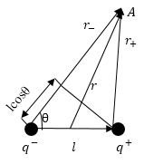
Рис. 1
Так как $lll r$, можно считать, что:
[r_—r_+approx lcostheta , r_-cdot r_+approx r^2left(3right).]
При этом местоположение точки A можно характеризовать вектором$overrightarrow{ r}$ с началом в любой точке диполя, ввиду малых геометрических размеров диполя. В таком случае формулу (2) можно записать в виде:
[varphi left(rright)=frac{1}{4pi {varepsilon }_0varepsilon }frac{overrightarrow{p_e}cdot overrightarrow{r}}{r^3}left(4right),]
где $qlcostheta =frac{overrightarrow{p_e}cdot overrightarrow{r}}{r}.$ Зная связь напряженности поля и потенциала:
[overrightarrow{E}=-gradvarphi (5)]
запишем формулу для напряженности поля диполя, которая будет иметь вид:
[overrightarrow{E}=frac{1}{4pi {varepsilon }_0varepsilon }left(frac{3left({overrightarrow{p}}_ecdot overrightarrow{r}right)overrightarrow{r}}{r^5}-frac{overrightarrow{p_e}}{r^3}right)left(6right).]
Согласно формуле (6) напряженность поля диполя убывает быстрее, чем напряженность кулоновского поля одиночного заряда, пропорционально третьей степени расстояния. Силовые линии электростатического поля около диполя изображены на рис. 2.
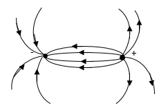
Рис. 2
Модуль вектора сопряженности
Если сферическую систему координат разместить так, чтобы ее центр совпал с серединой плеча диполя, а полярная ось была параллельна $overrightarrow{p_e}$ (рис.3), то составляющие вектора напряженности будут иметь вид:
[E_r=frac{1}{2pi {varepsilon }_0varepsilon }frac{p_ecos vartheta}{r^3},E_vartheta=frac{1}{4pi {varepsilon }_0varepsilon }frac{p_esin vartheta}{r^3},E_{varphi }=0. left(7right).]
В таком случае модуль вектора напряженности равен:
[E=frac{1}{4pi {varepsilon }_0varepsilon }frac{p_e}{r^3}sqrt{3{cos}^2vartheta+1}left(8right).]
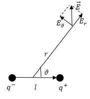
Рис. 3
Вычисление момента сил
В однородном поле сила, которая действует на диполь со стороны поля ($overrightarrow{F}$), равна нулю, так как к зарядам приложены одинаковые по модулю и противоположные по направлению силы:
[overrightarrow{F}={overrightarrow{F}}_++{overrightarrow{F}}_-=0left(9right),]
где ${overrightarrow{F}}_+$- сила, действующая на положительный заряд диполя, ${overrightarrow{F}}$ — сила, действующая на отрицательный заряд диполя.
Момент этих сил равен:
[overrightarrow{M}=overrightarrow{p_e}times overrightarrow{E}left(10right).]
Момент сил $overrightarrow{M}$ стремится повернуть ось диполя в направлении поля $overrightarrow{E}.$ Существует два положения равновесия диполя: диполь параллелен полю (устойчивое положение) и антипараллелен (неустойчивое положение).
Если поле не однородно, то сила (сумма сил действующих на положительный и отрицательный заряд) не равна нулю.$ overrightarrow{F}={overrightarrow{F}}_++{overrightarrow{F}}_-ne 0$. В этом случае сила равна:
[overrightarrow{F}=qleft({overrightarrow{E}}_+-{overrightarrow{E}}_-right)left(11right).]
В том случае, если мы имеем дело с точечным диполем (плечо диполя очень мало), то сила, действующая на диполь, может быть записана как:
[overrightarrow{F}=p_{ex}frac{partial overrightarrow{E}}{?x}+p_{ey}frac{partial overrightarrow{E}}{partial y}+p_{ez}frac{partial overrightarrow{E}}{partial z}left(12right).]
или, что то же самое, но короче:
[overrightarrow{F}=left(overrightarrow{p}overrightarrow{nabla }right)overrightarrow{E}left(13right).]
ДИПО́ЛЬ-ДИПО́ЛЬНОЕ ВЗАИМОДЕ́ЙСТВИЕ, взаимодействие частиц (или многочастичных систем), каждая из которых обладает дипольным моментом. Если два электрич. диполя с дипольными моментами $boldsymbol{p_1}$ и $boldsymbol {p_2}$ расположены на расстоянии $r$ друг от друга, то напряжённость $boldsymbol E$ электрич. поля, создаваемого первым диполем в точке, где находится второй диполь, равна $$boldsymbol E=frac{3boldsymbol r(boldsymbol p_1boldsymbol r)-boldsymbol p_1r^2}{r^5}.$$При этом со стороны поля $boldsymbol E$ на диполь действует не только сила, но также момент силы, стремящийся изменить направление дипольного момента. Энергия $W$ взаимодействия двух диполей с моментами $boldsymbol p_1$ и $boldsymbol p_2$ равна $$W=frac{(boldsymbol p_1 boldsymbol p_2)r^2-3(boldsymbol P_1 boldsymbol r)(boldsymbol p_2 boldsymbol r)}{r^5}.$$ Эта величина зависит от взаимного расположения дипольных моментов. Напр., если дипольные моменты $boldsymbol p_1$ и $boldsymbol p_2$ и вектор $boldsymbol r$ лежат на одной прямой, то энергия взаимодействия минимальна в случае, когда дипольные моменты параллельны. Если же дипольные моменты перпендикулярны вектору $boldsymbol r$, то минимальная энергия взаимодействия соответствует антипараллельному расположению дипольных моментов.
Те же самые соотношения имеют место и для магнитных дипольных моментов, достаточно в приведённых соотношениях заменить электрич. дипольные моменты $boldsymbol p_1$ и $boldsymbol p_2$ на магнитные дипольные моменты $boldsymbol M_1$ и $boldsymbol M_2$.
Bзаимодействие электрич. дипольных моментов оказывает влияние на процессы поляризации диэлектриков, в частности на поведение сегнетоэлектриков. Взаимодействие магнитных дипольных моментов определяет ряд свойств магнетиков, в частности их доменную структуру (см. Домены).
From Wikipedia, the free encyclopedia
An intermolecular force (IMF) (or secondary force) is the force that mediates interaction between molecules, including the electromagnetic forces of attraction
or repulsion which act between atoms and other types of neighbouring particles, e.g. atoms or ions. Intermolecular forces are weak relative to intramolecular forces – the forces which hold a molecule together. For example, the covalent bond, involving sharing electron pairs between atoms, is much stronger than the forces present between neighboring molecules. Both sets of forces are essential parts of force fields frequently used in molecular mechanics.
The first reference to the nature of microscopic forces is found in Alexis Clairaut’s work Théorie de la figure de la Terre, published in Paris in 1743.[1] Other scientists who have contributed to the investigation of microscopic forces include: Laplace, Gauss, Maxwell and Boltzmann.
Attractive intermolecular forces are categorized into the following types:
- Hydrogen bonding
- Ion–dipole forces and ion–induced dipole forces
- Van der Waals forces – Keesom force, Debye force, and London dispersion force
Information on intermolecular forces is obtained by macroscopic measurements of properties like viscosity, pressure, volume, temperature (PVT) data. The link to microscopic aspects is given by virial coefficients and Lennard-Jones potentials.
Hydrogen bonding[edit]
A hydrogen bond is an extreme form of dipole-dipole bonding, referring to the attraction between a hydrogen atom that is bonded to an element with high electronegativity, usually nitrogen, oxygen, or fluorine.[2] The hydrogen bond is often described as a strong electrostatic dipole–dipole interaction. However, it also has some features of covalent bonding: it is directional, stronger than a van der Waals force interaction, produces interatomic distances shorter than the sum of their van der Waals radii, and usually involves a limited number of interaction partners, which can be interpreted as a kind of valence. The number of Hydrogen bonds formed between molecules is equal to the number of active pairs. The molecule which donates its hydrogen is termed the donor molecule, while the molecule containing lone pair participating in H bonding is termed the acceptor molecule. The number of active pairs is equal to the common number between number of hydrogens the donor has and the number of lone pairs the acceptor has.

Hydrogen bonding in water
Though both not depicted in the diagram, water molecules have four active bonds. The oxygen atom’s two lone pairs interact with a hydrogen each, forming two additional hydrogen bonds, and the second hydrogen atom also interacts with a neighbouring oxygen. Intermolecular hydrogen bonding is responsible for the high boiling point of water (100 °C) compared to the other group 16 hydrides, which have little capability to hydrogen bond. Intramolecular hydrogen bonding is partly responsible for the secondary, tertiary, and quaternary structures of proteins and nucleic acids. It also plays an important role in the structure of polymers, both synthetic and natural.[3]
Beta bonding[edit]
The attraction between cationic and anionic sites is a noncovalent, or intermolecular interaction which is usually referred to as ion pairing or salt bridge.[4]
It is essentially due to electrostatic forces, although in aqueous medium the association is driven by entropy and often even endothermic. Most salts form crystals with characteristic distances between the ions; in contrast to many other noncovalent interactions, salt bridges are not directional and show in the solid state usually contact determined only by the van der Waals radii of the ions.
Inorganic as well as organic ions display in water at moderate ionic strength I similar salt bridge as association ΔG values around 5 to 6 kJ/mol for a 1:1 combination of anion and cation, almost independent of the nature (size, polarizability, etc.) of the ions.[5] The ΔG values are additive and approximately a linear function of the charges, the interaction of e.g. a doubly charged phosphate anion with a single charged ammonium cation accounts for about 2×5 = 10 kJ/mol. The ΔG values depend on the ionic strength I of the solution, as described by the Debye-Hückel equation, at zero ionic strength one observes ΔG = 8 kJ/mol.
Dipole–dipole and similar interactions [edit]
Dipole–dipole interactions (or Keesom interactions) are electrostatic interactions between molecules which have permanent dipoles. This interaction is stronger than the London forces but is weaker than ion-ion interaction because only partial charges are involved. These interactions tend to align the molecules to increase attraction (reducing potential energy). An example of a dipole–dipole interaction can be seen in hydrogen chloride (HCl): the positive end of a polar molecule will attract the negative end of the other molecule and influence its position. Polar molecules have a net attraction between them. Examples of polar molecules include hydrogen chloride (HCl) and chloroform (CHCl3).

Often molecules contain dipolar groups of atoms, but have no overall dipole moment on the molecule as a whole. This occurs if there is symmetry within the molecule that causes the dipoles to cancel each other out. This occurs in molecules such as tetrachloromethane and carbon dioxide. The dipole–dipole interaction between two individual atoms is usually zero, since atoms rarely carry a permanent dipole.
The Keesom interaction is a van der Waals force. It is discussed further in the section «Van der Waals forces».
Ion–dipole and ion–induced dipole forces[edit]
Ion–dipole and ion–induced dipole forces are similar to dipole–dipole and dipole–induced dipole interactions but involve ions, instead of only polar and non-polar molecules. Ion–dipole and ion–induced dipole forces are stronger than dipole–dipole interactions because the charge of any ion is much greater than the charge of a dipole moment. Ion–dipole bonding is stronger than hydrogen bonding.[6]
An ion–dipole force consists of an ion and a polar molecule interacting. They align so that the positive and negative groups are next to one another, allowing maximum attraction. An important example of this interaction is hydration of ions in water which give rise to hydration enthalpy. The polar water molecules surround themselves around ions in water and the energy released during the process is known as hydration enthalpy. The interaction has its immense importance in justifying the stability of various ions (like Cu2+) in water.
An ion–induced dipole force consists of an ion and a non-polar molecule interacting. Like a dipole–induced dipole force, the charge of the ion causes distortion of the electron cloud on the non-polar molecule.[7]
Van der Waals forces[edit]
The van der Waals forces arise from interaction between uncharged atoms or molecules, leading not only to such phenomena as the cohesion of condensed phases and physical absorption of gases, but also to a universal force of attraction between macroscopic bodies.[8]
Keesom force (permanent dipole – permanent dipole) [edit]
The first contribution to van der Waals forces is due to electrostatic interactions between rotating permanent dipoles, quadrupoles (all molecules with symmetry lower than cubic), and multipoles. It is termed the Keesom interaction, named after Willem Hendrik Keesom.[9] These forces originate from the attraction between permanent dipoles (dipolar molecules) and are temperature dependent.[8]
They consist of attractive interactions between dipoles that are ensemble averaged over different rotational orientations of the dipoles. It is assumed that the molecules are constantly rotating and never get locked into place. This is a good assumption, but at some point molecules do get locked into place. The energy of a Keesom interaction depends on the inverse sixth power of the distance, unlike the interaction energy of two spatially fixed dipoles, which depends on the inverse third power of the distance. The Keesom interaction can only occur among molecules that possess permanent dipole moments, i.e., two polar molecules. Also Keesom interactions are very weak van der Waals interactions and do not occur in aqueous solutions that contain electrolytes. The angle averaged interaction is given by the following equation:

where d = electric dipole moment,  = permitivity of free space,
  = dielectric constant of surrounding material, T = temperature,
  = Boltzmann constant, and r = distance between molecules.
Debye force (permanent dipoles–induced dipoles) [edit]
The second contribution is the induction (also termed polarization) or Debye force, arising from interactions between rotating permanent dipoles and from the polarizability of atoms and molecules (induced dipoles). These induced dipoles occur when one molecule with a permanent dipole repels another molecule’s electrons. A molecule with permanent dipole can induce a dipole in a similar neighboring molecule and cause mutual attraction. Debye forces cannot occur between atoms. The forces between induced and permanent dipoles are not as temperature dependent as Keesom interactions because the induced dipole is free to shift and rotate around the polar molecule. The Debye induction effects and Keesom orientation effects are termed polar interactions.[8]
The induced dipole forces appear from the induction (also termed polarization), which is the attractive interaction between a permanent multipole on one molecule with an induced (by the former di/multi-pole) 31 on another.[10][11][12] This interaction is called the Debye force, named after Peter J. W. Debye.
One example of an induction interaction between permanent dipole and induced dipole is the interaction between HCl and Ar. In this system, Ar experiences a dipole as its electrons are attracted (to the H side of HCl) or repelled (from the Cl side) by HCl.[10][11] The angle averaged interaction is given by the following equation:

where  = polarizability.
This kind of interaction can be expected between any polar molecule and non-polar/symmetrical molecule. The induction-interaction force is far weaker than dipole–dipole interaction, but stronger than the London dispersion force.
London dispersion force (fluctuating dipole–induced dipole interaction)[edit]
The third and dominant contribution is the dispersion or London force (fluctuating dipole–induced dipole), which arises due to the non-zero instantaneous dipole moments of all atoms and molecules. Such polarization can be induced either by a polar molecule or by the repulsion of negatively charged electron clouds in non-polar molecules. Thus, London interactions are caused by random fluctuations of electron density in an electron cloud. An atom with a large number of electrons will have a greater associated London force than an atom with fewer electrons. The dispersion (London) force is the most important component because all materials are polarizable, whereas Keesom and Debye forces require permanent dipoles. The London interaction is universal and is present in atom-atom interactions as well. For various reasons, London interactions (dispersion) have been considered relevant for interactions between macroscopic bodies in condensed systems. Hamaker developed the theory of van der Waals between macroscopic bodies in 1937 and showed that the additivity of these interactions renders them considerably more long-range.[8]
Relative strength of forces[edit]
| Bond type | Dissociation energy (kcal/mol)[13] |
Dissociation energy
(kJ/mol) |
Note |
|---|---|---|---|
| Ionic lattice | 250–4000[14] | 1100–20000 | |
| Covalent bond | 30–260 | 130–1100 | |
| Hydrogen bond | 1–12 | 4–50 | About 5 kcal/mol (21 kJ/mol) in water |
| Dipole–dipole | 0.5–2 | 2–8 | |
| London dispersion forces | <1 to 15 | <4 to 63 | Estimated from the enthalpies of vaporization of hydrocarbons[15] |
This comparison is approximate. The actual relative strengths will vary depending on the molecules involved. For instance, the presence of water creates competing interactions that greatly weaken the strength of both ionic and hydrogen bonds.[16] We may consider that for static systems, Ionic bonding and covalent bonding will always be stronger than intermolecular forces in any given substance. But it is not so for big moving systems like enzyme molecules interacting with substrate molecules.[17] Here the numerous intramolecular (most often — hydrogen bonds) bonds form an active intermediate state where the intermolecular bonds cause some of the covalent bond to be broken, while the others are formed, in this way procceding the thousands of enzymatic reactions, so important for living organisms.
Effect on the behavior of gases[edit]
Intermolecular forces are repulsive at short distances and attractive at long distances (see the Lennard-Jones potential). In a gas, the repulsive force chiefly has the effect of keeping two molecules from occupying the same volume. This gives a real gas a tendency to occupy a larger volume than an ideal gas at the same temperature and pressure. The attractive force draws molecules closer together and gives a real gas a tendency to occupy a smaller volume than an ideal gas. Which interaction is more important depends on temperature and pressure (see compressibility factor).
In a gas, the distances between molecules are generally large, so intermolecular forces have only a small effect. The attractive force is not overcome by the repulsive force, but by the thermal energy of the molecules. Temperature is the measure of thermal energy, so increasing temperature reduces the influence of the attractive force. In contrast, the influence of the repulsive force is essentially unaffected by temperature.
When a gas is compressed to increase its density, the influence of the attractive force increases. If the gas is made sufficiently dense, the attractions can become large enough to overcome the tendency of thermal motion to cause the molecules to disperse. Then the gas can condense to form a solid or liquid, i.e., a condensed phase. Lower temperature favors the formation of a condensed phase. In a condensed phase, there is very nearly a balance between the attractive and repulsive forces.
Quantum mechanical theories[edit]
Intermolecular forces observed between atoms and molecules can be described phenomenologically as occurring between permanent and instantaneous dipoles, as outlined above. Alternatively, one may seek a fundamental, unifying theory that is able to explain the various types of interactions such as hydrogen bonding,[18] van der Waals force[19] and dipole–dipole interactions. Typically, this is done by applying the ideas of quantum mechanics to molecules, and Rayleigh–Schrödinger perturbation theory has been especially effective in this regard. When applied to existing quantum chemistry methods, such a quantum mechanical explanation of intermolecular interactions provides an array of approximate methods that can be used to analyze intermolecular interactions.[20] One of the most helpful methods to visualize this kind of intermolecular interactions, that we can find in quantum chemistry, is the non-covalent interaction index, which is based on the electron density of the system. London dispersion forces play a big role with this.
Concerning electron density topology, recent methods based on electron density gradient methods have emerged recently, notably with the development of IBSI (Intrinsic Bond Strength Index),[21] relying on the IGM (Independent Gradient Model) methodology.[22][23][24]
See also[edit]
- Ionic bonding
- Salt bridges
- Coomber’s relationship
- Force field (chemistry)
- Hydrophobic effect
- Intramolecular force
- Molecular solid
- Polymer
- Quantum chemistry computer programs
- van der Waals force
- Comparison of software for molecular mechanics modeling
- Non-covalent interactions
- Solvation
References[edit]
- ^ Margenau H, Kestner NR (1969). Theory of Intermolecular Forces. International Series of Monographs in Natural Philosophy. Vol. 18 (1st ed.). Oxford: Pergamon Press. ISBN 978-0-08-016502-8.
- ^ IUPAC, Compendium of Chemical Terminology, 2nd ed. (the «Gold Book») (1997). Online corrected version: (2006–) «hydrogen bond». doi:10.1351/goldbook.H02899
- ^ Lindh U (2013), «Biological functions of the elements», in Selinus O (ed.), Essentials of Medical Geology (Revised ed.), Dordrecht: Springer, pp. 129–177, doi:10.1007/978-94-007-4375-5_7, ISBN 978-94-007-4374-8
- ^ Ciferri A, Perico A, eds. (2012). Ionic Interactions in Natural and Synthetic Macromolecules. Hoboken, NJ: John Wiley & Sons, Inc. ISBN 978-0-470-52927-0.
- ^ Biedermann F, Schneider HJ (May 2016). «Experimental Binding Energies in Supramolecular Complexes». Chemical Reviews. 116 (9): 5216–5300. doi:10.1021/acs.chemrev.5b00583. PMID 27136957.
- ^ Tro N (2011). Chemistry: A Molecular Approach. United States: Pearson Education Inc. p. 466. ISBN 978-0-321-65178-5.
- ^ Blaber M (1996). «Intermolecular Forces». mikeblaber.org. Archived from the original on 2020-08-01. Retrieved 2011-11-17.
- ^ a b c d Leite FL, Bueno CC, Da Róz AL, Ziemath EC, Oliveira ON (October 2012). «Theoretical models for surface forces and adhesion and their measurement using atomic force microscopy». International Journal of Molecular Sciences. 13 (10): 12773–12856. doi:10.3390/ijms131012773. PMC 3497299. PMID 23202925.
- ^ Keesom WH (1915). «The second virial coefficient for rigid spherical molecules whose mutual attraction is equivalent to that of a quadruplet placed at its center» (PDF). Proceedings of the Royal Netherlands Academy of Arts and Sciences. 18: 636–646.
- ^ a b Blustin PH (1978). «A Floating Gaussian Orbital calculation on argon hydrochloride (Ar·HCl)». Theoretica Chimica Acta. 47 (3): 249–257. doi:10.1007/BF00577166. S2CID 93104668.
- ^ a b Roberts JK, Orr WJ (1938). «Induced dipoles and the heat of adsorption of argon on ionic crystals». Transactions of the Faraday Society. 34: 1346. doi:10.1039/TF9383401346.
- ^ Sapse AM, Rayez-Meaume MT, Rayez JC, Massa LJ (1979). «Ion-induced dipole H−n clusters». Nature. 278 (5702): 332–333. Bibcode:1979Natur.278..332S. doi:10.1038/278332a0. S2CID 4304250.
- ^ Eğe SN (2004). Organic Chemistry: Structure and Reactivity (5th ed.). Boston: Houghton Mifflin Company. pp. 30–33, 67. ISBN 978-0-618-31809-4.
- ^ «Lattice Energies». Division of Chemical Education. Purdue University. Retrieved 2014-01-21.
- ^ Majer V, Svoboda V (1985). Enthalpies of Vaporization of Organic Compounds. Oxford: Blackwell Scientific. ISBN 978-0-632-01529-0.
- ^ Alberts B (2015). Molecular biology of the cell (6th ed.). New York, NY. ISBN 978-0-8153-4432-2. OCLC 887605755.
- ^ Savir Y, Tlusty T (May 2007). «Conformational proofreading: the impact of conformational changes on the specificity of molecular recognition». PLOS ONE. 2 (5): e468. Bibcode:2007PLoSO…2..468S. doi:10.1371/journal.pone.0000468. PMC 1868595. PMID 17520027.
- ^ Arunan E, Desiraju GR, Klein RA, Sadlej J, Scheiner S, Alkorta I, et al. (2011-07-08). «Definition of the hydrogen bond (IUPAC Recommendations 2011)». Pure and Applied Chemistry. 83 (8): 1637–1641. doi:10.1351/PAC-REC-10-01-02. ISSN 1365-3075. S2CID 97688573.
- ^ Landau LD, Lifshitz EM (1960). Electrodynamics of Continuous Media. Oxford: Pergamon. pp. 368–376.
- ^ King M (1976). «Theory of the Chemical Bond». JACS. 98 (12): 3415–3420. doi:10.1021/ja00428a004.
- ^ Klein J, Khartabil H, Boisson JC, Contreras-García J, Piquemal JP, Hénon E (March 2020). «New Way for Probing Bond Strength» (PDF). The Journal of Physical Chemistry A. 124 (9): 1850–1860. Bibcode:2020JPCA..124.1850K. doi:10.1021/acs.jpca.9b09845. PMID 32039597. S2CID 211070812.
- ^ Lefebvre C, Rubez G, Khartabil H, Boisson JC, Contreras-García J, Hénon E (July 2017). «Accurately extracting the signature of intermolecular interactions present in the NCI plot of the reduced density gradient versus electron density» (PDF). Physical Chemistry Chemical Physics. 19 (27): 17928–17936. Bibcode:2017PCCP…1917928L. doi:10.1039/C7CP02110K. PMID 28664951.
- ^ Lefebvre C, Khartabil H, Boisson JC, Contreras-García J, Piquemal JP, Hénon E (March 2018). «The Independent Gradient Model: A New Approach for Probing Strong and Weak Interactions in Molecules from Wave Function Calculations» (PDF). ChemPhysChem. 19 (6): 724–735. doi:10.1002/cphc.201701325. PMID 29250908.
- ^ Ponce-Vargas M, Lefebvre C, Boisson JC, Hénon E (January 2020). «Atomic Decomposition Scheme of Noncovalent Interactions Applied to Host-Guest Assemblies». Journal of Chemical Information and Modeling. 60 (1): 268–278. doi:10.1021/acs.jcim.9b01016. PMID 31877034. S2CID 209488458.