Как найти сингулярное разложение матрицы

Материал из MachineLearning.

Перейти к: навигация, поиск

Сингулярное разложение (Singular Value Decomposition, SVD) —
декомпозиция вещественной матрицы с целью ее приведения к каноническому виду.
Сингулярное разложение является удобным методом при работе с матрицами.
Оно показывает геометрическую структуру матрицы и позволяет наглядно представить имеющиеся данные.
Сингулярное разложение используется при решении самых разных задач —
от приближения методом наименьших квадратов и решения систем уравнений
до сжатия изображений.
При этом используются разные свойства сингулярного разложения, например,
способность показывать ранг матрицы, приближать матрицы данного ранга.
SVD позволяет вычислять обратные и псевдообратные матрицы большого размера,
что делает его полезным инструментом при решении задач регрессионного анализа.

Для любой вещественной -матрицы  существуют две вещественные
ортогональные -матрицы  и  такие,
что  — диагональная матрица ,

Матрицы  и  выбираются так, чтобы диагональные элементы матрицы  имели вид

где  — ранг матрицы . В частности, если  невырождена,

то

Индекс  элемента  есть фактическая размерность собственного пространства матрицы  .

Столбцы матриц  и  называются соответственно левыми и правыми сингулярными векторами, а значения диагонали матрицы  называются сингулярными числами.

Эквивалентная запись сингулярного разложения — .

Например, матрица

имеет сингулярное разложение

Легко увидеть, что матрицы  и  ортогональны,

также

и сумма квадратов значений их столбцов равна единице.

Геометрический смысл SVD

Пусть матрице  поставлен в соответствие линейный оператор.
Cингулярное разложение можно переформулировать в геометрических терминах.
Линейный оператор, отображающий элементы пространства  в себя представим в виде последовательно выполняемых
линейных операторов вращения, растяжения и вращения.
Поэтому компоненты сингулярного разложения наглядно показывают
геометрические изменения при отображении линейным оператором
множества векторов из векторного пространства в себя или в векторное пространство другой размерности.

Пространства матрицы и SVD

Сингулярное разложение позволяет найти ортогональные базисы
различных векторных пространств разлагаемой матрицы

Для прямоугольных матриц существует так называемое экономное представление сингулярного
разложения матрицы.

Согласно этому представлению при , диагональная
матрица  имеет пустые строки (их элементы равны нулю), а при  — пустые
столбцы. Поэтому существует еще одно экономное представление

в котором .

Нуль-пространство матрицы  — набор векторов , для
которого справедливо высказывание . Собственное
пространство матрицы  — набор векторов , при
котором уравнение  имеет ненулевое решение
для . Обозначим  и  — столбцы матриц  и .
Тогда разложение  может быть записано в виде:
, где . Если
сингулярное число , то и
находится в нуль-пространстве матрицы , а если
сингулярное число , то вектор  находятся в
собственном пространстве матрицы . Следовательно, можно
сконструировать базисы для различных векторных подпространств,
определенных матрицей . Hабор
векторов  в векторном
пространстве  формирует базис для , если любой
вектор  из  можно представить в виде линейной комбинации
векторов  единственным способом.
Пусть  будет набором тех столбцов , для
которых , а  — все остальные
столбцы . Также, пусть  будет набором столбцов ,
для которых , а  — все остальные
столбцы , включая и те, для которых . Тогда,
если  — количество ненулевых сингулярных чисел, то
имеется  столбцов в наборе  и  столбцов в
наборе  и , а также  столбцов в наборе .
Каждый из этих наборов формирует базис векторного пространства матрицы :

SVD и собственные числа матрицы

Сингулярное разложение обладает свойством, которое связывает
задачу отыскания сингулярного разложения и задачу отыскания
собственных векторов. Собственный вектор  матрицы  —
такой вектор, при котором выполняется условие ,
число  называется собственным числом. Так как матрицы 
и  ортогональные, то

Умножая оба выражения справа соответственно на  и  получаем

Из этого следует, что столбцы матрицы  являются собственными
векторами матрицы , а квадраты сингулярных чисел
 — ее собственными
числами.
Также столбцы матрицы являются собственными векторами матрицы , а
квадраты сингулярных чисел являются ее собственными числами.

SVD и норма матриц

Рассмотрим изменение длины вектора  до и после его умножения
слева на матрицу . Евклидова норма вектора определена как

Если матрица  ортогональна, длина вектора  остается неизменной. В противном
случае можно вычислить, насколько матрица  растянула
вектор .

Евклидова норма матрицы есть максимальный коэффициент растяжения произвольного вектора  заданной матрицей 

Альтернативой Евклидовой норме является норма Фробениуса:

Если известно сингулярное разложение, то обе эти нормы легко
вычислить. Пусть  — сингулярные числа матрицы , отличные от нуля.
Тогда

и

Сингулярные числа матрицы  — это длины осей эллипсоида,
заданного множеством

Нахождение псевдообратной матрицы с помощью SVD

Если -матрица  является вырожденной или
прямоугольной, то обратной матрицы  для нее не существует.
Однако для  может быть найдена псевдообратная

матрица  — такая матрица, для которой выполняются условия

Пусть найдено разложение матрицы  вида

где

, и
.
Тогда матрица  является для матрицы 
псевдообратной.
Действительно, , .

Метод наименьших квадратов и число обусловленности

Задача наименьших квадратов ставится следующим образом. Даны
действительная -матрица  и
действительный -вектор . Требуется найти
действительный -вектор , минимизирующий Евклидову длину

вектора невязки,

Решение

задачи наименьших квадратов —

Для отыскания решения  требуется обратить матрицу .
Для квадратных матриц  число обусловленности  определено отношением

Из формулы Евклидовой нормы матрицы и предыдущей формулы следует, что число обусловленности матрицы есть отношение ее первого сингулярного числа к последнему.

Следовательно, число обусловленности матрицы  есть квадрат числа обусловленности матрицы .
Это высказывание справедливо и для вырожденных матриц, если полагать число обусловленности как отношение
,  — ранг матрицы .
Поэтому для получения обращения, устойчивого к малым изменениям значений матрицы , используется усеченное SVD.

Усеченное SVD при обращении матриц

Пусть матрица  представлена в виде .
Тогда при нахождении обратной матрицы
в силу ортогональности матриц  и  и в силу условия убывания диагональных элементов
матрицы ,
псевдообратная матрица  будет более зависеть от тех элементов
матрицы , которые имеют меньшие значения, чем от первых
сингулярных чисел. Действительно, если матрица  имеет сингулярные числа
, то
сингулярные числа матрицы  равны

и

Считая первые  сингулярных чисел определяющими собственное
пространство матрицы , используем при обращении матрицы 
первые  сингулярных чисел, . Тогда обратная матрица  будет
найдена как .

Определим усеченную псевдообратную матрицу  как

где  —
-диагональная матрица.

Смотри также

• Метод главных компонент
• Простой итерационный алгоритм сингулярного разложения
• Регрессионный анализ
• Интегральный индикатор
• Согласование экспертных оценок

Литература

• Голуб Дж., Ван-Лоун Ч. Матричные вычисления. М.: Мир. 1999.
• Деммель Дж. Вычислительная линейная алгебра. URSS. 2001.
• Логинов Н.В. Сингулярное разложение матриц. М.: МГАПИ. 1996.
• Стренг Г. Линейная алгебра и ее применения. М.: Мир. 1980.
• Форсайт Дж., Молер К. Численное решение систем линейных алгебраических уравнений. М.: Мир. 1969.
• Хорн Р., Джонсон Ч. Матричный анализ. М.: Мир. 1989.
• Vetterling W. T. Flannery B. P. Numerical Recipies in C: The Art of Scientific Computing. NY: Cambridge University Press. 1999.
• Meltzer T. SVD and its Application to Generalized Eigenvalue Problems. 2004. 16 pages.

In linear algebra, the singular value decomposition (SVD) is a factorization of a real or complex matrix. It generalizes the eigendecomposition of a square normal matrix with an orthonormal eigenbasis to any matrix. It is related to the polar decomposition.

Specifically, the singular value decomposition of an complex matrix M is a factorization of the form where U is an complex unitary matrix, is an rectangular diagonal matrix with non-negative real numbers on the diagonal, V is an complex unitary matrix, and is the conjugate transpose of V. Such decomposition always exists for any complex matrix. If M is real, then U and V can be guaranteed to be real orthogonal matrices; in such contexts, the SVD is often denoted

The diagonal entries of are uniquely determined by M and are known as the singular values of M. The number of non-zero singular values is equal to the rank of M. The columns of U and the columns of V are called left-singular vectors and right-singular vectors of M, respectively. They form two sets of orthonormal bases u₁, …, u_m and v₁, …, v_n , and if they are sorted so that the singular values with value zero are all in the highest-numbered columns (or rows), the singular value decomposition can be written as where is the rank of M.

The SVD is not unique. It is always possible to choose the decomposition so that the singular values are in descending order. In this case, (but not U and V) is uniquely determined by M.

The term sometimes refers to the compact SVD, a similar decomposition in which is square diagonal of size , where is the rank of M, and has only the non-zero singular values. In this variant, U is an semi-unitary matrix and is an semi-unitary matrix, such that

Mathematical applications of the SVD include computing the pseudoinverse, matrix approximation, and determining the rank, range, and null space of a matrix. The SVD is also extremely useful in all areas of science, engineering, and statistics, such as signal processing, least squares fitting of data, and process control.

Intuitive interpretations[edit]

Rotation, coordinate scaling, and reflection[edit]

In the special case when M is an m × m real square matrix, the matrices U and V^⁎ can be chosen to be real m × m matrices too. In that case, «unitary» is the same as «orthogonal». Then, interpreting both unitary matrices as well as the diagonal matrix, summarized here as A, as a linear transformation x ↦ Ax of the space R^m, the matrices U and V^⁎ represent rotations or reflection of the space, while represents the scaling of each coordinate x_i by the factor σ_i. Thus the SVD decomposition breaks down any linear transformation of R^m into a composition of three geometrical transformations: a rotation or reflection (V^⁎), followed by a coordinate-by-coordinate scaling (), followed by another rotation or reflection (U).

In particular, if M has a positive determinant, then U and V^⁎ can be chosen to be both rotations with reflections, or both rotations without reflections.^{[citation needed]} If the determinant is negative, exactly one of them will have a reflection. If the determinant is zero, each can be independently chosen to be of either type.

If the matrix M is real but not square, namely m×n with m ≠ n, it can be interpreted as a linear transformation from Rⁿ to R^m. Then U and V^⁎ can be chosen to be rotations/reflections of R^m and Rⁿ, respectively; and , besides scaling the first coordinates, also extends the vector with zeros, i.e. removes trailing coordinates, so as to turn Rⁿ into R^m.

Singular values as semiaxes of an ellipse or ellipsoid[edit]

As shown in the figure, the singular values can be interpreted as the magnitude of the semiaxes of an ellipse in 2D. This concept can be generalized to n-dimensional Euclidean space, with the singular values of any n × n square matrix being viewed as the magnitude of the semiaxis of an n-dimensional ellipsoid. Similarly, the singular values of any m × n matrix can be viewed as the magnitude of the semiaxis of an n-dimensional ellipsoid in m-dimensional space, for example as an ellipse in a (tilted) 2D plane in a 3D space. Singular values encode magnitude of the semiaxis, while singular vectors encode direction. See below for further details.

The columns of U and V are orthonormal bases[edit]

Since U and V^⁎ are unitary, the columns of each of them form a set of orthonormal vectors, which can be regarded as basis vectors. The matrix M maps the basis vector V_i to the stretched unit vector σ_i U_i. By the definition of a unitary matrix, the same is true for their conjugate transposes U^⁎ and V, except the geometric interpretation of the singular values as stretches is lost. In short, the columns of U, U^⁎, V, and V^⁎ are orthonormal bases. When is a positive-semidefinite Hermitian matrix, U and V are both equal to the unitary matrix used to diagonalize . However, when is not positive-semidefinite and Hermitian but still diagonalizable, its eigendecomposition and singular value decomposition are distinct.

Geometric meaning[edit]

Because U and V are unitary, we know that the columns U₁, …, U_m of U yield an orthonormal basis of K^m and the columns V₁, …, V_n of V yield an orthonormal basis of Kⁿ (with respect to the standard scalar products on these spaces).

The linear transformation

has a particularly simple description with respect to these orthonormal bases: we have

where σ_i is the i-th diagonal entry of , and T(V_i) = 0 for i > min(m,n).

The geometric content of the SVD theorem can thus be summarized as follows: for every linear map T : Kⁿ → K^m one can find orthonormal bases of Kⁿ and K^m such that T maps the i-th basis vector of Kⁿ to a non-negative multiple of the i-th basis vector of K^m, and sends the left-over basis vectors to zero. With respect to these bases, the map T is therefore represented by a diagonal matrix with non-negative real diagonal entries.

To get a more visual flavor of singular values and SVD factorization – at least when working on real vector spaces – consider the sphere S of radius one in Rⁿ. The linear map T maps this sphere onto an ellipsoid in R^m. Non-zero singular values are simply the lengths of the semi-axes of this ellipsoid. Especially when n = m, and all the singular values are distinct and non-zero, the SVD of the linear map T can be easily analyzed as a succession of three consecutive moves: consider the ellipsoid T(S) and specifically its axes; then consider the directions in Rⁿ sent by T onto these axes. These directions happen to be mutually orthogonal. Apply first an isometry V^⁎ sending these directions to the coordinate axes of Rⁿ. On a second move, apply an endomorphism D diagonalized along the coordinate axes and stretching or shrinking in each direction, using the semi-axes lengths of T(S) as stretching coefficients. The composition D ∘ V^⁎ then sends the unit-sphere onto an ellipsoid isometric to T(S). To define the third and last move, apply an isometry U to this ellipsoid to obtain T(S). As can be easily checked, the composition U ∘ D ∘ V^⁎ coincides with T.

Example[edit]

Consider the 4 × 5 matrix

A singular value decomposition of this matrix is given by UΣV^⁎

The scaling matrix is zero outside of the diagonal (grey italics) and one diagonal element is zero (red bold, light blue bold in dark mode). Furthermore, because the matrices U and V^⁎ are unitary, multiplying by their respective conjugate transposes yields identity matrices, as shown below. In this case, because U and V^⁎ are real valued, each is an orthogonal matrix.

This particular singular value decomposition is not unique. Choosing such that

is also a valid singular value decomposition.

SVD and spectral decomposition[edit]

Singular values, singular vectors, and their relation to the SVD[edit]

A non-negative real number σ is a singular value for M if and only if there exist unit-length vectors in K^m and in Kⁿ such that

The vectors and are called left-singular and right-singular vectors for σ, respectively.

In any singular value decomposition

the diagonal entries of are equal to the singular values of M. The first p = min(m, n) columns of U and V are, respectively, left- and right-singular vectors for the corresponding singular values. Consequently, the above theorem implies that:

• An m × n matrix M has at most p distinct singular values.
• It is always possible to find a unitary basis U for K^m with a subset of basis vectors spanning the left-singular vectors of each singular value of M.
• It is always possible to find a unitary basis V for Kⁿ with a subset of basis vectors spanning the right-singular vectors of each singular value of M.

A singular value for which we can find two left (or right) singular vectors that are linearly independent is called degenerate. If and are two left-singular vectors which both correspond to the singular value σ, then any normalized linear combination of the two vectors is also a left-singular vector corresponding to the singular value σ. The similar statement is true for right-singular vectors. The number of independent left and right-singular vectors coincides, and these singular vectors appear in the same columns of U and V corresponding to diagonal elements of all with the same value σ.

As an exception, the left and right-singular vectors of singular value 0 comprise all unit vectors in the cokernel and kernel, respectively, of M, which by the rank–nullity theorem cannot be the same dimension if m ≠ n. Even if all singular values are nonzero, if m > n then the cokernel is nontrivial, in which case U is padded with m − n orthogonal vectors from the cokernel. Conversely, if m < n, then V is padded by n − m orthogonal vectors from the kernel. However, if the singular value of 0 exists, the extra columns of U or V already appear as left or right-singular vectors.

Non-degenerate singular values always have unique left- and right-singular vectors, up to multiplication by a unit-phase factor e^iφ (for the real case up to a sign). Consequently, if all singular values of a square matrix M are non-degenerate and non-zero, then its singular value decomposition is unique, up to multiplication of a column of U by a unit-phase factor and simultaneous multiplication of the corresponding column of V by the same unit-phase factor.
In general, the SVD is unique up to arbitrary unitary transformations applied uniformly to the column vectors of both U and V spanning the subspaces of each singular value, and up to arbitrary unitary transformations on vectors of U and V spanning the kernel and cokernel, respectively, of M.

Relation to eigenvalue decomposition[edit]

The singular value decomposition is very general in the sense that it can be applied to any m × n matrix, whereas eigenvalue decomposition can only be applied to diagonalizable matrices. Nevertheless, the two decompositions are related.

Given an SVD of M, as described above, the following two relations hold:

The right-hand sides of these relations describe the eigenvalue decompositions of the left-hand sides. Consequently:

• The columns of V (right-singular vectors) are eigenvectors of M^⁎M.
• The columns of U (left-singular vectors) are eigenvectors of MM^⁎.
• The non-zero elements of (non-zero singular values) are the square roots of the non-zero eigenvalues of M^⁎M or MM^⁎.

In the special case that M is a normal matrix, which by definition must be square, the spectral theorem says that it can be unitarily diagonalized using a basis of eigenvectors, so that it can be written M = UDU^⁎ for a unitary matrix U and a diagonal matrix D with complex elements σ_i along the diagonal. When M is positive semi-definite, σ_i will be non-negative real numbers so that the decomposition M = UDU^⁎ is also a singular value decomposition. Otherwise, it can be recast as an SVD by moving the phase e^iφ of each σ_i to either its corresponding V_i or U_i. The natural connection of the SVD to non-normal matrices is through the polar decomposition theorem: M = SR, where S = UΣU^⁎ is positive semidefinite and normal, and R = UV^⁎ is unitary.

Thus, except for positive semi-definite matrices, the eigenvalue decomposition and SVD of M, while related, differ: the eigenvalue decomposition is M = UDU⁻¹, where U is not necessarily unitary and D is not necessarily positive semi-definite, while the SVD is M = UΣV^⁎, where is diagonal and positive semi-definite, and U and V are unitary matrices that are not necessarily related except through the matrix M. While only non-defective square matrices have an eigenvalue decomposition, any matrix has a SVD.

Applications of the SVD[edit]

Pseudoinverse[edit]

The singular value decomposition can be used for computing the pseudoinverse of a matrix. (Various authors use different notation for the pseudoinverse; here we use ^†.) Indeed, the pseudoinverse of the matrix M with singular value decomposition M = UΣV^⁎ is

M^† = V Σ^† U^⁎

where Σ^† is the pseudoinverse of Σ, which is formed by replacing every non-zero diagonal entry by its reciprocal and transposing the resulting matrix. The pseudoinverse is one way to solve linear least squares problems.

Solving homogeneous linear equations[edit]

A set of homogeneous linear equations can be written as Ax = 0 for a matrix A and vector x. A typical situation is that A is known and a non-zero x is to be determined which satisfies the equation. Such an x belongs to A‘s null space and is sometimes called a (right) null vector of A. The vector x can be characterized as a right-singular vector corresponding to a singular value of A that is zero. This observation means that if A is a square matrix and has no vanishing singular value, the equation has no non-zero x as a solution. It also means that if there are several vanishing singular values, any linear combination of the corresponding right-singular vectors is a valid solution. Analogously to the definition of a (right) null vector, a non-zero x satisfying x^⁎A = 0, with x^⁎ denoting the conjugate transpose of x, is called a left null vector of A.

Total least squares minimization[edit]

A total least squares problem seeks the vector x that minimizes the 2-norm of a vector Ax under the constraint ||x|| = 1. The solution turns out to be the right-singular vector of A corresponding to the smallest singular value.

Range, null space and rank[edit]

Another application of the SVD is that it provides an explicit representation of the range and null space of a matrix M. The right-singular vectors corresponding to vanishing singular values of M span the null space of M and the left-singular vectors corresponding to the non-zero singular values of M span the range of M. For example, in the above example the null space is spanned by the last two rows of V^⁎ and the range is spanned by the first three columns of U.

As a consequence, the rank of M equals the number of non-zero singular values which is the same as the number of non-zero diagonal elements in . In numerical linear algebra the singular values can be used to determine the effective rank of a matrix, as rounding error may lead to small but non-zero singular values in a rank deficient matrix. Singular values beyond a significant gap are assumed to be numerically equivalent to zero.

Low-rank matrix approximation[edit]

Some practical applications need to solve the problem of approximating a matrix M with another matrix , said to be truncated, which has a specific rank r. In the case that the approximation is based on minimizing the Frobenius norm of the difference between M and under the constraint that , it turns out that the solution is given by the SVD of M, namely

where is the same matrix as except that it contains only the r largest singular values (the other singular values are replaced by zero). This is known as the Eckart–Young theorem, as it was proved by those two authors in 1936 (although it was later found to have been known to earlier authors; see Stewart 1993).

Separable models[edit]

The SVD can be thought of as decomposing a matrix into a weighted, ordered sum of separable matrices. By separable, we mean that a matrix A can be written as an outer product of two vectors A = u ⊗ v, or, in coordinates, . Specifically, the matrix M can be decomposed as

Here U_i and V_i are the i-th columns of the corresponding SVD matrices, σ_i are the ordered singular values, and each A_i is separable. The SVD can be used to find the decomposition of an image processing filter into separable horizontal and vertical filters. Note that the number of non-zero σ_i is exactly the rank of the matrix.

Separable models often arise in biological systems, and the SVD factorization is useful to analyze such systems. For example, some visual area V1 simple cells’ receptive fields can be well described^[1] by a Gabor filter in the space domain multiplied by a modulation function in the time domain. Thus, given a linear filter evaluated through, for example, reverse correlation, one can rearrange the two spatial dimensions into one dimension, thus yielding a two-dimensional filter (space, time) which can be decomposed through SVD. The first column of U in the SVD factorization is then a Gabor while the first column of V represents the time modulation (or vice versa). One may then define an index of separability

which is the fraction of the power in the matrix M which is accounted for by the first separable matrix in the decomposition.^[2]

Nearest orthogonal matrix[edit]

It is possible to use the SVD of a square matrix A to determine the orthogonal matrix O closest to A. The closeness of fit is measured by the Frobenius norm of O − A. The solution is the product UV^⁎.^[3] This intuitively makes sense because an orthogonal matrix would have the decomposition UIV^⁎ where I is the identity matrix, so that if A = UΣV^⁎ then the product A = UV^⁎ amounts to replacing the singular values with ones. Equivalently, the solution is the unitary matrix R = UV^⁎ of the Polar Decomposition M = RP = P‘R in either order of stretch and rotation, as described above.

A similar problem, with interesting applications in shape analysis, is the orthogonal Procrustes problem, which consists of finding an orthogonal matrix O which most closely maps A to B. Specifically,

where denotes the Frobenius norm.

This problem is equivalent to finding the nearest orthogonal matrix to a given matrix M = A^TB.

The Kabsch algorithm[edit]

The Kabsch algorithm (called Wahba’s problem in other fields) uses SVD to compute the optimal rotation (with respect to least-squares minimization) that will align a set of points with a corresponding set of points. It is used, among other applications, to compare the structures of molecules.

Signal processing[edit]

The SVD and pseudoinverse have been successfully applied to signal processing,^[4] image processing^[5] and big data (e.g., in genomic signal processing).^[6][7][8][9]

Astrodynamics[edit]

In Astrodynamics, the SVD and its variants are used as an option to determine suitable maneuver directions for transfer trajectory design^[10] and Orbital station-keeping.^[11]

Other examples[edit]

The SVD is also applied extensively to the study of linear inverse problems and is useful in the analysis of regularization methods such as that of Tikhonov. It is widely used in statistics, where it is related to principal component analysis and to correspondence analysis, and in signal processing and pattern recognition. It is also used in output-only modal analysis, where the non-scaled mode shapes can be determined from the singular vectors. Yet another usage is latent semantic indexing in natural-language text processing.

In general numerical computation involving linear or linearized systems, there is a universal constant that characterizes the regularity or singularity of a problem, which is the system’s «condition number» . It often controls the error rate or convergence rate of a given computational scheme on such systems.^[12][13]

The SVD also plays a crucial role in the field of quantum information, in a form often referred to as the Schmidt decomposition. Through it, states of two quantum systems are naturally decomposed, providing a necessary and sufficient condition for them to be entangled: if the rank of the matrix is larger than one.

One application of SVD to rather large matrices is in numerical weather prediction, where Lanczos methods are used to estimate the most linearly quickly growing few perturbations to the central numerical weather prediction over a given initial forward time period; i.e., the singular vectors corresponding to the largest singular values of the linearized propagator for the global weather over that time interval. The output singular vectors in this case are entire weather systems. These perturbations are then run through the full nonlinear model to generate an ensemble forecast, giving a handle on some of the uncertainty that should be allowed for around the current central prediction.

SVD has also been applied to reduced order modelling. The aim of reduced order modelling is to reduce the number of degrees of freedom in a complex system which is to be modeled. SVD was coupled with radial basis functions to interpolate solutions to three-dimensional unsteady flow problems.^[14]

Interestingly, SVD has been used to improve gravitational waveform modeling by the ground-based gravitational-wave interferometer aLIGO.^[15] SVD can help to increase the accuracy and speed of waveform generation to support gravitational-waves searches and update two different waveform models.

Singular value decomposition is used in recommender systems to predict people’s item ratings.^[16] Distributed algorithms have been developed for the purpose of calculating the SVD on clusters of commodity machines.^[17]

Low-rank SVD has been applied for hotspot detection from spatiotemporal data with application to disease outbreak detection.^[18] A combination of SVD and higher-order SVD also has been applied for real time event detection from complex data streams (multivariate data with space and time dimensions) in disease surveillance.^[19]

Proof of existence[edit]

An eigenvalue λ of a matrix M is characterized by the algebraic relation Mu = λu. When M is Hermitian, a variational characterization is also available. Let M be a real n × n symmetric matrix. Define

By the extreme value theorem, this continuous function attains a maximum at some u when restricted to the unit sphere {||x|| = 1}. By the Lagrange multipliers theorem, u necessarily satisfies

for some real number λ. The nabla symbol, ∇, is the del operator (differentiation with respect to x). Using the symmetry of M we obtain

Therefore Mu = λu, so u is a unit length eigenvector of M. For every unit length eigenvector v of M its eigenvalue is f(v), so λ is the largest eigenvalue of M. The same calculation performed on the orthogonal complement of u gives the next largest eigenvalue and so on. The complex Hermitian case is similar; there f(x) = x* M x is a real-valued function of 2n real variables.

Singular values are similar in that they can be described algebraically or from variational principles. Although, unlike the eigenvalue case, Hermiticity, or symmetry, of M is no longer required.

This section gives these two arguments for existence of singular value decomposition.

Based on the spectral theorem[edit]

Let be an m × n complex matrix. Since is positive semi-definite and Hermitian, by the spectral theorem, there exists an n × n unitary matrix such that

where is diagonal and positive definite, of dimension , with the number of non-zero eigenvalues of (which can be shown to verify ). Note that is here by definition a matrix whose -th column is the -th eigenvector of , corresponding to the eigenvalue . Moreover, the -th column of , for , is an eigenvector of with eigenvalue . This can be expressed by writing as , where the columns of and therefore contain the eigenvectors of corresponding to non-zero and zero eigenvalues, respectively. Using this rewriting of , the equation becomes:

This implies that

Moreover, the second equation implies .^[20] Finally, the unitary-ness of translates, in terms of and , into the following conditions:

where the subscripts on the identity matrices are used to remark that they are of different dimensions.

Let us now define

Then,

since This can be also seen as immediate consequence of the fact that . This is equivalent to the observation that if is the set of eigenvectors of corresponding to non-vanishing eigenvalues , then is a set of orthogonal vectors, and is a (generally not complete) set of orthonormal vectors. This matches with the matrix formalism used above denoting with the matrix whose columns are , with the matrix whose columns are the eigenvectors of with vanishing eigenvalue, and the matrix whose columns are the vectors .

We see that this is almost the desired result, except that and are in general not unitary, since they might not be square. However, we do know that the number of rows of is no smaller than the number of columns, since the dimensions of is no greater than and . Also, since

the columns in are orthonormal and can be extended to an orthonormal basis. This means that we can choose such that is unitary.

For V₁ we already have V₂ to make it unitary. Now, define

where extra zero rows are added or removed to make the number of zero rows equal the number of columns of U₂, and hence the overall dimensions of equal to . Then

which is the desired result:

Notice the argument could begin with diagonalizing MM^⁎ rather than M^⁎M (This shows directly that MM^⁎ and M^⁎M have the same non-zero eigenvalues).

Based on variational characterization[edit]

The singular values can also be characterized as the maxima of u^TMv, considered as a function of u and v, over particular subspaces. The singular vectors are the values of u and v where these maxima are attained.

Let M denote an m × n matrix with real entries. Let S^k−1 be the unit -sphere in , and define

Consider the function σ restricted to S^m−1 × Sⁿ⁻¹. Since both S^m−1 and Sⁿ⁻¹ are compact sets, their product is also compact. Furthermore, since σ is continuous, it attains a largest value for at least one pair of vectors u ∈ S^m−1 and v ∈ Sⁿ⁻¹. This largest value is denoted σ₁ and the corresponding vectors are denoted u₁ and v₁. Since σ₁ is the largest value of σ(u, v) it must be non-negative. If it were negative, changing the sign of either u₁ or v₁ would make it positive and therefore larger.

Statement. u₁, v₁ are left and right-singular vectors of M with corresponding singular value σ₁.

Proof. Similar to the eigenvalues case, by assumption the two vectors satisfy the Lagrange multiplier equation:

After some algebra, this becomes

Multiplying the first equation from left by and the second equation from left by and taking ||u|| = ||v|| = 1 into account gives

Plugging this into the pair of equations above, we have

This proves the statement.

More singular vectors and singular values can be found by maximizing σ(u, v) over normalized u, v which are orthogonal to u₁ and v₁, respectively.

The passage from real to complex is similar to the eigenvalue case.

Calculating the SVD[edit]

The singular value decomposition can be computed using the following observations:

• The left-singular vectors of M are a set of orthonormal eigenvectors of MM^⁎.
• The right-singular vectors of M are a set of orthonormal eigenvectors of M^⁎M.
• The non-zero singular values of M (found on the diagonal entries of ) are the square roots of the non-zero eigenvalues of both M^⁎M and MM^⁎.

Numerical approach[edit]

The SVD of a matrix M is typically computed by a two-step procedure. In the first step, the matrix is reduced to a bidiagonal matrix. This takes O(mn²) floating-point operations (flop), assuming that m ≥ n. The second step is to compute the SVD of the bidiagonal matrix. This step can only be done with an iterative method (as with eigenvalue algorithms). However, in practice it suffices to compute the SVD up to a certain precision, like the machine epsilon. If this precision is considered constant, then the second step takes O(n) iterations, each costing O(n) flops. Thus, the first step is more expensive, and the overall cost is O(mn²) flops (Trefethen & Bau III 1997, Lecture 31).

The first step can be done using Householder reflections for a cost of 4mn² − 4n³/3 flops, assuming that only the singular values are needed and not the singular vectors. If m is much larger than n then it is advantageous to first reduce the matrix M to a triangular matrix with the QR decomposition and then use Householder reflections to further reduce the matrix to bidiagonal form; the combined cost is 2mn² + 2n³ flops (Trefethen & Bau III 1997, Lecture 31).

The second step can be done by a variant of the QR algorithm for the computation of eigenvalues, which was first described by Golub & Kahan (1965). The LAPACK subroutine DBDSQR^[21] implements this iterative method, with some modifications to cover the case where the singular values are very small (Demmel & Kahan 1990). Together with a first step using Householder reflections and, if appropriate, QR decomposition, this forms the DGESVD^[22] routine for the computation of the singular value decomposition.

The same algorithm is implemented in the GNU Scientific Library (GSL). The GSL also offers an alternative method that uses a one-sided Jacobi orthogonalization in step 2 (GSL Team 2007). This method computes the SVD of the bidiagonal matrix by solving a sequence of 2 × 2 SVD problems, similar to how the Jacobi eigenvalue algorithm solves a sequence of 2 × 2 eigenvalue methods (Golub & Van Loan 1996, §8.6.3). Yet another method for step 2 uses the idea of divide-and-conquer eigenvalue algorithms (Trefethen & Bau III 1997, Lecture 31).

There is an alternative way that does not explicitly use the eigenvalue decomposition.^[23] Usually the singular value problem of a matrix M is converted into an equivalent symmetric eigenvalue problem such as M M^⁎, M^⁎M, or

The approaches that use eigenvalue decompositions are based on the QR algorithm, which is well-developed to be stable and fast.
Note that the singular values are real and right- and left- singular vectors are not required to form similarity transformations. One can iteratively alternate between the QR decomposition and the LQ decomposition to find the real diagonal Hermitian matrices. The QR decomposition gives M ⇒ Q R and the LQ decomposition of R gives R ⇒ L P^⁎. Thus, at every iteration, we have M ⇒ Q L P^⁎, update M ⇐ L and repeat the orthogonalizations. Eventually,^{[clarification needed]} this iteration between QR decomposition and LQ decomposition produces left- and right- unitary singular matrices. This approach cannot readily be accelerated, as the QR algorithm can with spectral shifts or deflation. This is because the shift method is not easily defined without using similarity transformations. However, this iterative approach is very simple to implement, so is a good choice when speed does not matter. This method also provides insight into how purely orthogonal/unitary transformations can obtain the SVD.

Analytic result of 2 × 2 SVD[edit]

The singular values of a 2 × 2 matrix can be found analytically. Let the matrix be

where are complex numbers that parameterize the matrix, I is the identity matrix, and denote the Pauli matrices. Then its two singular values are given by

Reduced SVDs[edit]

In applications it is quite unusual for the full SVD, including a full unitary decomposition of the null-space of the matrix, to be required. Instead, it is often sufficient (as well as faster, and more economical for storage) to compute a reduced version of the SVD. The following can be distinguished for an m×n matrix M of rank r:

Thin SVD[edit]

The thin, or economy-sized, SVD of a matrix M is given by^[24]

where

,

the matrices U_k and V_k contain only the first k columns of U and V, and Σ_k contains only the first k singular values from Σ. The matrix U_k is thus m×k, Σ_k is k×k diagonal, and V_k* is k×n.

The thin SVD uses significantly less space and computation time if k ≪ max(m, n). The first stage in its calculation will usually be a QR decomposition of M, which can make for a significantly quicker calculation in this case.

Compact SVD[edit]

Only the r column vectors of U and r row vectors of V* corresponding to the non-zero singular values Σ_r are calculated. The remaining vectors of U and V* are not calculated. This is quicker and more economical than the thin SVD if r ≪ min(m, n). The matrix U_r is thus m×r, Σ_r is r×r diagonal, and V_r* is r×n.

Truncated SVD[edit]

In many applications the number r of the non-zero singular values is large making even the Compact SVD impractical to compute. In such cases, the smallest singular values may need to be truncated to compute only t ≪ r non-zero singular values. The truncated SVD is no longer an exact decomposition of the original matrix M, but rather provides the optimal low-rank matrix approximation by any matrix of a fixed rank t

,

where matrix U_t is m×t, Σ_t is t×t diagonal, and V_t* is t×n.
Only the t column vectors of U and t row vectors of V* corresponding to the t largest singular values Σ_t are calculated. This can be much quicker and more economical than the compact SVD if t≪r, but requires a completely different toolset of numerical solvers.

In applications that require an approximation to the Moore–Penrose inverse of the matrix M, the smallest singular values of M are of interest, which are more challenging to compute compared to the largest ones.

Truncated SVD is employed in latent semantic indexing.^[25]

Norms[edit]

Ky Fan norms[edit]

The sum of the k largest singular values of M is a matrix norm, the Ky Fan k-norm of M.^[26]

The first of the Ky Fan norms, the Ky Fan 1-norm, is the same as the operator norm of M as a linear operator with respect to the Euclidean norms of K^m and Kⁿ. In other words, the Ky Fan 1-norm is the operator norm induced by the standard ℓ² Euclidean inner product. For this reason, it is also called the operator 2-norm. One can easily verify the relationship between the Ky Fan 1-norm and singular values. It is true in general, for a bounded operator M on (possibly infinite-dimensional) Hilbert spaces

But, in the matrix case, (M* M)^1/2 is a normal matrix, so ||M* M||^1/2 is the largest eigenvalue of (M* M)^1/2, i.e. the largest singular value of M.

The last of the Ky Fan norms, the sum of all singular values, is the trace norm (also known as the ‘nuclear norm’), defined by ||M|| = Tr[(M* M)^1/2] (the eigenvalues of M* M are the squares of the singular values).

Hilbert–Schmidt norm[edit]

The singular values are related to another norm on the space of operators. Consider the Hilbert–Schmidt inner product on the n × n matrices, defined by

So the induced norm is

Since the trace is invariant under unitary equivalence, this shows

where σ_i are the singular values of M. This is called the Frobenius norm, Schatten 2-norm, or Hilbert–Schmidt norm of M. Direct calculation shows that the Frobenius norm of M = (m_ij) coincides with:

In addition, the Frobenius norm and the trace norm (the nuclear norm) are special cases of the Schatten norm.

Variations and generalizations[edit]

Scale-invariant SVD[edit]

The singular values of a matrix A are uniquely defined and are invariant with respect to left and/or right unitary transformations of A. In other words, the singular values of UAV, for unitary U and V, are equal to the singular values of A. This is an important property for applications in which it is necessary to preserve Euclidean distances and invariance with respect to rotations.

The Scale-Invariant SVD, or SI-SVD,^[27] is analogous to the conventional SVD except that its uniquely-determined singular values are invariant with respect to diagonal transformations of A. In other words, the singular values of DAE, for invertible diagonal matrices D and E, are equal to the singular values of A. This is an important property for applications for which invariance to the choice of units on variables (e.g., metric versus imperial units) is needed.

Bounded operators on Hilbert spaces[edit]

The factorization M = UΣV^⁎ can be extended to a bounded operator M on a separable Hilbert space H. Namely, for any bounded operator M, there exist a partial isometry U, a unitary V, a measure space (X, μ), and a non-negative measurable f such that

where is the multiplication by f on L²(X, μ).

This can be shown by mimicking the linear algebraic argument for the matricial case above. VT_fV* is the unique positive square root of M*M, as given by the Borel functional calculus for self-adjoint operators. The reason why U need not be unitary is because, unlike the finite-dimensional case, given an isometry U₁ with nontrivial kernel, a suitable U₂ may not be found such that

is a unitary operator.

As for matrices, the singular value factorization is equivalent to the polar decomposition for operators: we can simply write

and notice that U V* is still a partial isometry while VT_fV* is positive.

Singular values and compact operators[edit]

The notion of singular values and left/right-singular vectors can be extended to compact operator on Hilbert space as they have a discrete spectrum. If T is compact, every non-zero λ in its spectrum is an eigenvalue. Furthermore, a compact self-adjoint operator can be diagonalized by its eigenvectors. If M is compact, so is M^⁎M. Applying the diagonalization result, the unitary image of its positive square root T_f  has a set of orthonormal eigenvectors {e_i} corresponding to strictly positive eigenvalues {σ_i}. For any ψ ∈ H,

where the series converges in the norm topology on H. Notice how this resembles the expression from the finite-dimensional case. σ_i are called the singular values of M. {Ue_i} (resp. {Ve_i}) can be considered the left-singular (resp. right-singular) vectors of M.

Compact operators on a Hilbert space are the closure of finite-rank operators in the uniform operator topology. The above series expression gives an explicit such representation. An immediate consequence of this is:

Theorem. M is compact if and only if M^⁎M is compact.

History[edit]

The singular value decomposition was originally developed by differential geometers, who wished to determine whether a real bilinear form could be made equal to another by independent orthogonal transformations of the two spaces it acts on. Eugenio Beltrami and Camille Jordan discovered independently, in 1873 and 1874 respectively, that the singular values of the bilinear forms, represented as a matrix, form a complete set of invariants for bilinear forms under orthogonal substitutions. James Joseph Sylvester also arrived at the singular value decomposition for real square matrices in 1889, apparently independently of both Beltrami and Jordan. Sylvester called the singular values the canonical multipliers of the matrix A. The fourth mathematician to discover the singular value decomposition independently is Autonne in 1915, who arrived at it via the polar decomposition. The first proof of the singular value decomposition for rectangular and complex matrices seems to be by Carl Eckart and Gale J. Young in 1936;^[28] they saw it as a generalization of the principal axis transformation for Hermitian matrices.

In 1907, Erhard Schmidt defined an analog of singular values for integral operators (which are compact, under some weak technical assumptions); it seems he was unaware of the parallel work on singular values of finite matrices. This theory was further developed by Émile Picard in 1910, who is the first to call the numbers singular values (or in French, valeurs singulières).

Practical methods for computing the SVD date back to Kogbetliantz in 1954–1955 and Hestenes in 1958,^[29] resembling closely the Jacobi eigenvalue algorithm, which uses plane rotations or Givens rotations. However, these were replaced by the method of Gene Golub and William Kahan published in 1965,^[30] which uses Householder transformations or reflections. In 1970, Golub and Christian Reinsch^[31] published a variant of the Golub/Kahan algorithm that is still the one most-used today.

See also[edit]

Notes[edit]

References[edit]

• Banerjee, Sudipto; Roy, Anindya (2014), Linear Algebra and Matrix Analysis for Statistics, Texts in Statistical Science (1st ed.), Chapman and Hall/CRC, ISBN 978-1420095388
• Chicco, D; Masseroli, M (2015). «Software suite for gene and protein annotation prediction and similarity search». IEEE/ACM Transactions on Computational Biology and Bioinformatics. 12 (4): 837–843. doi:10.1109/TCBB.2014.2382127. hdl:11311/959408. PMID 26357324. S2CID 14714823.
• Trefethen, Lloyd N.; Bau III, David (1997). Numerical linear algebra. Philadelphia: Society for Industrial and Applied Mathematics. ISBN 978-0-89871-361-9.
• Demmel, James; Kahan, William (1990). «Accurate singular values of bidiagonal matrices». SIAM Journal on Scientific and Statistical Computing. 11 (5): 873–912. CiteSeerX 10.1.1.48.3740. doi:10.1137/0911052.
• Golub, Gene H.; Kahan, William (1965). «Calculating the singular values and pseudo-inverse of a matrix». Journal of the Society for Industrial and Applied Mathematics, Series B: Numerical Analysis. 2 (2): 205–224. Bibcode:1965SJNA….2..205G. doi:10.1137/0702016. JSTOR 2949777.
• Golub, Gene H.; Van Loan, Charles F. (1996). Matrix Computations (3rd ed.). Johns Hopkins. ISBN 978-0-8018-5414-9.
• GSL Team (2007). «§14.4 Singular Value Decomposition». GNU Scientific Library. Reference Manual.
• Halldor, Bjornsson and Venegas, Silvia A. (1997). «A manual for EOF and SVD analyses of climate data». McGill University, CCGCR Report No. 97-1, Montréal, Québec, 52pp.
• Hansen, P. C. (1987). «The truncated SVD as a method for regularization». BIT. 27 (4): 534–553. doi:10.1007/BF01937276. S2CID 37591557.
• Horn, Roger A.; Johnson, Charles R. (1985). «Section 7.3». Matrix Analysis. Cambridge University Press. ISBN 978-0-521-38632-6.
• Horn, Roger A.; Johnson, Charles R. (1991). «Chapter 3». Topics in Matrix Analysis. Cambridge University Press. ISBN 978-0-521-46713-1.
• Samet, H. (2006). Foundations of Multidimensional and Metric Data Structures. Morgan Kaufmann. ISBN 978-0-12-369446-1.
• Strang G. (1998). «Section 6.7». Introduction to Linear Algebra (3rd ed.). Wellesley-Cambridge Press. ISBN 978-0-9614088-5-5.
• Stewart, G. W. (1993). «On the Early History of the Singular Value Decomposition». SIAM Review. 35 (4): 551–566. CiteSeerX 10.1.1.23.1831. doi:10.1137/1035134. hdl:1903/566. JSTOR 2132388.
• Wall, Michael E.; Rechtsteiner, Andreas; Rocha, Luis M. (2003). «Singular value decomposition and principal component analysis». In D.P. Berrar; W. Dubitzky; M. Granzow (eds.). A Practical Approach to Microarray Data Analysis. Norwell, MA: Kluwer. pp. 91–109.
• Press, WH; Teukolsky, SA; Vetterling, WT; Flannery, BP (2007), «Section 2.6», Numerical Recipes: The Art of Scientific Computing (3rd ed.), New York: Cambridge University Press, ISBN 978-0-521-88068-8

External links[edit]

• Online SVD calculator

Время на прочтение
6 мин

Количество просмотров 4.5K

Привет, Хабр! Меня зовут Илья Котов, я Data Scientist в Сбере, участник профессионального сообщества NTA. Эта статья — первая часть небольшого цикла, посвящённого алгоритмам вложения вершин графа в векторное пространство. Сегодня расскажу об алгоритмах, основанных на матричных факторизациях. В качестве примера в статье используется занимательная задача поиска сообществ в графе. Что же, приступим!

Начнём с постановки задачи

Давайте представим, что в школе X учится старшеклассник, который создал собственную социальную сеть. Всю школу поразила его изобретательность, все пытаются стать пользователями его творения. На переменах (а иногда и на уроках) то и дело обсуждают его продукт плюс активно используют, непрерывно нажимая указательным пальцем на экран телефона.

Автор проекта понимает, что его пользовательская база стала достаточно большой, пользователи приходят уже из других школ, а школьники из кружков по программированию присылают свои резюме для участия в развитии социальной сети. Но успех не будет вечен, людей необходимо удерживать новым функционалом и возможностями.

Тогда голову старшеклассника посетила гениальная мысль: «А почему бы не сделать систему, которая будет рекомендовать вашему пользователю потенциального друга?» Но как это сделать?

На примере этой задачи я разберу алгоритмы вложений графов, основанные на матричном разложении, чтобы впоследствии вы смогли использовать эти алгоритмы и для своих прикладных задач. Приступим.

Разрабатываем алгоритм рекомендации «друзей» в социальной сети

 Нечто подобное вы могли видеть в vk.com.

Программисты из VK, безусловно, никогда не раскроют алгоритм рекомендации, но примерный принцип работы алгоритма понятен.

Вероятно, друг — это человек, с которым у вас есть что-то общее, возможно, хобби, работа, место учёбы, музыкальные предпочтения. Продолжать можно до бесконечности.

Как правило (но необязательно), вы знакомы с друзьями своего друга или даже с друзьями друга вашего друга. Также, скорее всего, у вас и вашего друга есть много общих друзей и знакомых. Соответственно, друзья и знакомые находятся примерно в общем социальном окружении, социальном кластере.

Зачем нам графы?

Теперь вернёмся к проекту нашего старшеклассника. В мире, полном сложных структур и закономерностей, ему нужен гибкий инструмент, который позволяет в достаточной мере хранить в себе информацию для последующего анализа. Графы — один из вариантов, который может решить эту задачу и помочь юному разработчику обрести ещё большую популярность.

Общество очень удобно моделировать с помощью графа, его приложение вы точно встретите в социологии. Давайте считать вершинами графа пользователей, а отношения между этими вершинами будут только в том случае, если (пользователь X *дружит* с пользователем Y). Отношения обладают свойством симметричности (для нашего случая), то есть это означает, что если (пользователь X *дружит* с пользователем Y), то и (пользователь Y *дружит* с пользователем X). Это в идеальном мире, а вот в реальной жизни такая система не всегда работает.

В качестве набора данных выступает граф дружбы выборки пользователей из социальной сети Facebook (данные были анонимизированы, источник — Stanford Large Network Dataset Collection).

Как анализировать эти графы? Хотелось бы применять привычные и всеми любимые алгоритмы машинного обучения, нейросети и статистику, но уже к данным, представленным в виде графа. На самом деле старшекласснику не нужно изобретать что-то новое, требуется лишь найти способ перейти из вершин и отношений в обычное векторное пространство, сохраняя при этом топологию графа. Эти векторы дадут возможность использовать инструменты, перечисленные выше, в том числе и алгоритмы кластеризации, для нахождения кластеров вершин, это и нужно старшекласснику.

Матрица смежности приходит на помощь

Матрица смежности — довольно простой, но мощный инструмент.

Формальное определение звучит так:

Матрица смежности графа G — квадратная матрица размера N × N,где N-количество вершин графа G, в которой значение элемента A(i,j) равно числу рёбер из i вершины графа в j-ую.

В самом простом случае неориентированного графа — это симметричная матрица, заполненная нулями и единицами. 

Старшеклассник выгрузил данные пользователей из соседних классов, и вот что у него получилось:

import networkx as nx
import matplotlib.pyplot as plt
%matplotlib inline
plt.figure(figsize=(10, 5))
graph = nx.Graph()
graph.add_edges_from(data)
plt.subplot(1, 2, 1)
nx.draw(graph)
plt.subplot(1, 2, 2)
plt.imshow(nx.adjacency_matrix(graph).toarray())

Жёлтый цвет означает единицу (то есть существует связь), тёмно-фиолетовый означает ноль (отсутствие связи).

Несложно заметить, что граф имеет 2 выраженные группы и 1 группу, которая их соединяет. В этом графе всё просто и наглядно, он является скорее примером для понимания, чем реальной задачей с неочевидной структурой.

Если вы посмотрите на строки этой матрицы как на векторы, то они уже могут характеризовать вершины графа.

Сингулярное разложение матрицы

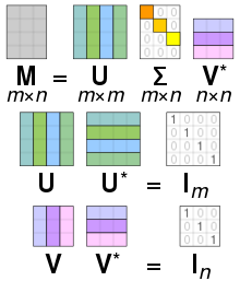
SVD (Singular Value Decomposition) — крайне важный и красивый факт линейной алгебры. Это представление прямоугольной матрицы в виде произведения трёх матриц особого вида (обычно пишут U S V^t).

Чтобы разложить матрицу через SVD, вы можете использовать пакет из библиотеки numpy, называется он linalg.

import numpy as np

U, S, V_t = np.linalg.svd(X)

У сингулярного разложения есть наглядный геометрический смысл. Матрицы U и V (левые и правые сингулярные векторы) — унитарные матрицы (более общий случай ортогональных матриц, то есть они совершают повороты в пространстве или выворачивают его, в случае отрицательного детерминанта, сохраняя длину векторов), а S — это диагональная матрица, элементы на диагонали — сингулярные значения (то есть геометрически она совершает функцию масштабирования).

Теперь применим это к матрице смежности. Роль векторов вершин будут исполнять строки матрицы U. Так как сингулярные числа в диагональной матрице S идут по убыванию (то есть s1>s2.. > sn), можно отбросить последние столбцы матрицы U (если быть точнее, то последние сингулярные векторы матрицы U), потому что они имеют небольшой вклад в формирование матрицы, а места занимают много. Это в целом проблема для больших графов, где очень много вершин, а связей мало, матрица смежности становится разреженной. Такие графы лучше представлять в виде простого списка отношений. Сингулярное разложение матрицы тем и удобно, что даёт представление об общей структуре, помогает понять геометрический смысл, найти шумы и оставить только самые весомые признаки.

(значения на главной диагонали матрицы S)

Пусть r = 2, для того, чтобы была возможность визуализировать данные на плоскости.

На изображении видно, что часть информации утеряна, однако чётко выделяются 3 группы.

Вот как изменяется детализация матрицы смежности в зависимости от параметра r.  

plt.figure(figsize=(15, 5))

for i in range(1, 19):

            plt.subplot(2, 9, i)

            plt.title(‘r=’ + str(i))

            plt.imshow(U[:, :i] @ np.diag(S[:i]) @ V_t[:i, :])

Визуализируем векторы матрицы U(nx2).

Алгоритм готов!

Наконец, у старшеклассника есть всё необходимое, и он готов перевернуть индустрию.

Вот что нужно сделать:

1. Найти матрицу смежности.

2. Разложить её с помощью SVD и обрезать столбцы матрицы левых сингулярных векторов.

3. Применить какой-нибудь алгоритм кластеризации.

Граф имеет довольно непростую структуру (см. первую картинку), однако всё равно различимы некоторые группы. Из-за сложности данных из матрицы левых сингулярных векторов нужно брать гораздо больше столбцов, чем в простейшем случае с двумя классами (в этом примере возьмём 100), иначе теряется  очень много информации.

import networkx as nx

import numpy as np

from sklearn.manifold import TSNE

#создадим простой граф и заполним его данными

graph = nx.Graph()

graph.add_edges_from(relations) #relations — это список, где элементом является кортеж вида ('n1', 'n2')

#матрица смежности

adj_matrix = nx.adjacency_matrix(graph)

#svd разложение

u, sigma, v_t = np.linalg.svd(adj_matrix.toarray())

#обрежем матрицу левых сингулярных векторов до 100

large_vectors = u[:, :100]

#снизим размерность до двух компонент для визуализации

emb = TSNE(n_components=2).fit_transform(large_vectors)

Далее используем алгоритм DBSCAN для кластеризации. Кластер, в котором находится пользователь, — это его социальное окружение. Людей, которые входят в него и при этом не дружат (не имеют контактов в социальной сети) с нашим пользователем, я и буду предлагать в качестве возможного друга или знакомого. Система довольно простая, но вы можете её расширять, например, обращать внимание на интересы пользователя, на какие группы он подписан, какую музыку слушает, где живёт и так далее, делая систему всё более эффективной.

from sklearn.cluster import DBSCAN

import seaborn as sns

df_scatterplot = pd.DataFrame(emb, columns=['e1', 'e2'])

df_scatterplot['label'] = DBSCAN(eps=2, min_samples=2).fit(emb).labels_

plt.figure(figsize=(10, 10))

sns.scatterplot(data=df_scatterplot, x='e1', y='e2', hue='label', s=8, palette='deep')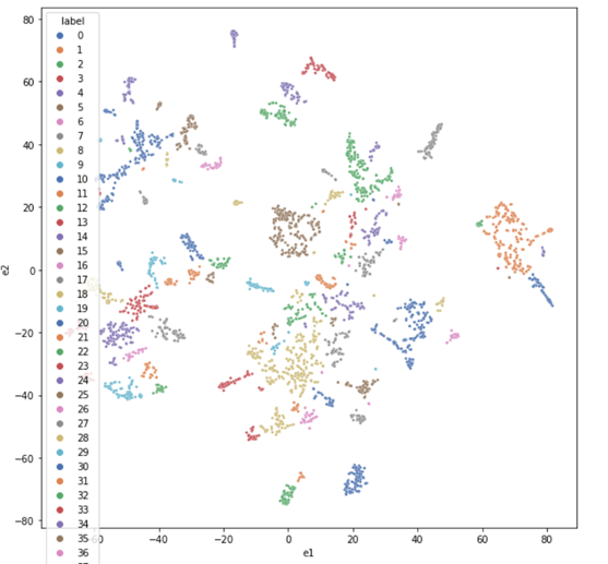

Собственно, на этом всё, конец первой части. Напомню, что сегодня я разобрал простой, но эффективный алгоритм, который может быть применён для ваших рабочих задач, где требуется анализ данных, представленных в виде графа. Алгоритмы, основанные на матричных факторизациях, обобщаются и на мультиграфы, только речь будет идти уже о тензорной факторизации (см. DistMult и т. п.). В следующей части я рассмотрю не менее интересные алгоритмы, основанные на случайных блужданиях.

Если у вас во время прочтения статьи возникли вопросы, задавайте их в комментариях, постараюсь ответить на все. А если вы работаете с алгоритмами рекомендаций и у вас есть предложения, пишите, обсудим.

Нежное введение в разложение по сингулярным числам для машинного обучения

  Перевод

  Ссылка на автора

Матричная декомпозиция, также известная как матричная факторизация, включает описание данной матрицы с использованием ее составляющих элементов.

Возможно, самый известный и широко используемый метод декомпозиции матрицы — это декомпозиция по сингулярному значению, или SVD. Все матрицы имеют SVD, что делает его более стабильным, чем другие методы, такие как собственное разложение. Как таковой, он часто используется в широком спектре приложений, включая сжатие, удаление шума и уменьшение объема данных.

В этом уроке вы обнаружите метод разложения по сингулярным значениям для разложения матрицы на составляющие ее элементы.

После завершения этого урока вы узнаете:

• Что такое разложение по сингулярному значению и что в нем участвует.
• Как рассчитать SVD и восстановить прямоугольную и квадратную матрицу из элементов SVD.
• Как рассчитать псевдообратное и выполнить уменьшение размерности, используя SVD.

Давайте начнем.

• Обновление март / 2018: Исправлена ​​опечатка в реконструкции. Для ясности изменено V в коде на VT. Исправлена ​​опечатка в псевдообратном уравнении.

Обзор учебника

Этот урок состоит из 5 частей; они есть:

1. Разложение по сингулярному значению
2. Рассчитать разложение по сингулярному значению
3. Восстановить Матрицу из СВД
4. СВД для псевдообратного
5. SVD для уменьшения размерности

Разложение по сингулярному значению

Разложение по сингулярному значению, или сокращенно SVD, — это метод разложения матрицы, предназначенный для сведения матрицы к ее составным частям, чтобы упростить некоторые последующие вычисления матрицы.

Для случая простоты мы сосредоточимся на SVD для вещественных матриц и проигнорируем случай для комплексных чисел.

A = U . Sigma . V^T

Где A — действительная матрица mxn, которую мы хотим разложить, U — матрица mxm, Sigma (часто представляемая заглавной греческой буквой Sigma) — диагональная матрица mxn, а V ^ T — транспонирование матрицы nxn, где T верхний индекс.

Разложение по сингулярным значениям является основным моментом линейной алгебры.

— страница 371, Введение в линейную алгебру, Пятое издание, 2016.

Диагональные значения в сигма-матрице называются сингулярными значениями исходной матрицы A. Столбцы матрицы U называются лево-сингулярными векторами A, а столбцы V называются правосингулярными векторами A.

SVD рассчитывается с помощью итерационных численных методов. Мы не будем вдаваться в подробности этих методов. Каждая прямоугольная матрица имеет разложение по сингулярным значениям, хотя результирующие матрицы могут содержать комплексные числа, а ограничения арифметики с плавающей запятой могут привести к тому, что некоторые матрицы не будут аккуратно разлагаться.

Разложение по сингулярным значениям (SVD) предоставляет еще один способ разложить матрицу на сингулярные векторы и сингулярные значения. SVD позволяет нам обнаруживать некоторую информацию того же вида, что и собственное разложение. Тем не менее, SVD является более общим.

— страницы 44-45, Глубокое обучение, 2016

SVD широко используется как при вычислении других матричных операций, таких как обратная матрица, так и в качестве метода сокращения данных в машинном обучении. SVD также может быть использован в линейной регрессии наименьших квадратов, сжатии изображений и шумоподавлении данных.

Декомпозиция сингулярных значений (SVD) имеет множество применений в статистике, машинном обучении и информатике. Нанесение SVD на матрицу похоже на рентгеновское зрение …

— Страница 297, Руководство по линейной алгебре, 2017

Рассчитать разложение по сингулярному значению

SVD можно рассчитать, вызвав функцию svd ().

Функция принимает матрицу и возвращает элементы U, Sigma и V ^ T. Диагональная матрица Сигмы возвращается как вектор сингулярных значений. Матрица V возвращается в транспонированной форме, например, Электронная лампа

В приведенном ниже примере определяется матрица 3 × 2 и вычисляется разложение по сингулярному значению.

# Singular-value decomposition
from numpy import array
from scipy.linalg import svd
# define a matrix
A = array([[1, 2], [3, 4], [5, 6]])
print(A)
# SVD
U, s, VT = svd(A)
print(U)
print(s)
print(VT)

При выполнении примера сначала печатается определенная матрица 3 × 2, затем матрица 3 × 3 U, вектор Sigma с 2 элементами и матричные элементы 2 × 2 V ^ T, вычисленные из разложения.

[[1 2]
 [3 4]
 [5 6]]

[[-0.2298477   0.88346102  0.40824829]
 [-0.52474482  0.24078249 -0.81649658]
 [-0.81964194 -0.40189603  0.40824829]]

[ 9.52551809  0.51430058]

[[-0.61962948 -0.78489445]
 [-0.78489445  0.61962948]]

Восстановить Матрицу из СВД

Исходная матрица может быть восстановлена ​​из элементов U, Sigma и V ^ T.

Элементы U, s и V, возвращаемые из svd (), не могут быть умножены напрямую.

Вектор s должен быть преобразован в диагональную матрицу с помощью функции diag (). По умолчанию эта функция создаст квадратную матрицу размером m x m относительно нашей исходной матрицы. Это вызывает проблему, поскольку размеры матриц не соответствуют правилам умножения матриц, где число столбцов в матрице должно соответствовать количеству строк в последующей матрице.

После создания квадратной диагональной матрицы Сигмы размеры матриц соответствуют исходной матрице m x n, которую мы разлагаем, следующим образом:

U (m x m) . Sigma (m x m) . V^T (n x n)

Где, на самом деле, мы требуем:

U (m x m) . Sigma (m x n) . V^T (n x n)

Мы можем достичь этого путем создания новой сигма-матрицы со всеми нулевыми значениями, которая равна m x n (например, больше строк), и заполнить первую n x n часть матрицы квадратной диагональной матрицей, вычисленной с помощью diag ().

# Reconstruct SVD
from numpy import array
from numpy import diag
from numpy import dot
from numpy import zeros
from scipy.linalg import svd
# define a matrix
A = array([[1, 2], [3, 4], [5, 6]])
print(A)
# Singular-value decomposition
U, s, VT = svd(A)
# create m x n Sigma matrix
Sigma = zeros((A.shape[0], A.shape[1]))
# populate Sigma with n x n diagonal matrix
Sigma[:A.shape[1], :A.shape[1]] = diag(s)
# reconstruct matrix
B = U.dot(Sigma.dot(VT))
print(B)

При выполнении примера сначала печатается исходная матрица, а затем матрица, восстановленная из элементов SVD.

[[1 2]
 [3 4]
 [5 6]]

[[ 1.  2.]
 [ 3.  4.]
 [ 5.  6.]]

Вышеупомянутое усложнение с диагональю сигмы существует только в случае, когда m и n не равны. Диагональная матрица может быть использована непосредственно при восстановлении квадратной матрицы следующим образом.

# Reconstruct SVD
from numpy import array
from numpy import diag
from numpy import dot
from scipy.linalg import svd
# define a matrix
A = array([[1, 2, 3], [4, 5, 6], [7, 8, 9]])
print(A)
# Singular-value decomposition
U, s, VT = svd(A)
# create n x n Sigma matrix
Sigma = diag(s)
# reconstruct matrix
B = U.dot(Sigma.dot(VT))
print(B)

При выполнении примера печатается исходная матрица 3 × 3 и версия, восстановленная непосредственно из элементов SVD.

[[1 2 3]
 [4 5 6]
 [7 8 9]]

[[ 1.  2.  3.]
 [ 4.  5.  6.]
 [ 7.  8.  9.]]

СВД для псевдообратного

Псевдообращение — это обобщение обратной матрицы для квадратных матриц на прямоугольные матрицы, где число строк и столбцов не равно.

Он также называется инверсией Мура-Пенроуза после двух независимых исследователей метода или Обобщенной инверсией.

Инверсия матриц не определена для матриц, которые не являются квадратными. […] Когда A имеет больше столбцов, чем строк, то решение линейного уравнения с использованием псевдообратного представления дает одно из многих возможных решений.

— страница 46, Глубокое обучение, 2016

Псевдообращение обозначается как A ^ +, где A — это инвертируемая матрица, а + — верхний индекс.

Псевдообращение вычисляется с использованием сингулярного разложения A:

A^+ = V . D^+ . U^T

Или без точечной записи:

A^+ = VD^+U^T

Где A ^ + — псевдообратная, D ^ + — псевдообратная диагональная матрица Sigma, а U ^ T — транспонирование U.

Мы можем получить U и V из операции SVD.

A = U . Sigma . V^T

D ^ + можно рассчитать путем создания диагональной матрицы из Sigma, вычисления обратной величины каждого ненулевого элемента в Sigma и выполнения транспонирования, если исходная матрица была прямоугольной.

s11,   0,   0
Sigma = (  0, s22,   0)
           0,   0, s33

1/s11,     0,     0
D^+ = (    0, 1/s22,     0)
           0,     0, 1/s33

Псевдообращение обеспечивает один из способов решения уравнения линейной регрессии, в частности, когда строк больше, чем столбцов, что часто имеет место.

NumPy предоставляет функцию pinv () для вычисления псевдообращения прямоугольной матрицы.

Пример ниже определяет матрицу 4 × 2 и вычисляет псевдообратную форму.

# Pseudoinverse
from numpy import array
from numpy.linalg import pinv
# define matrix
A = array([
	[0.1, 0.2],
	[0.3, 0.4],
	[0.5, 0.6],
	[0.7, 0.8]])
print(A)
# calculate pseudoinverse
B = pinv(A)
print(B)

При выполнении примера сначала печатается определенная матрица, а затем вычисленная псевдообратная.

[[ 0.1  0.2]
 [ 0.3  0.4]
 [ 0.5  0.6]
 [ 0.7  0.8]]

[[ -1.00000000e+01  -5.00000000e+00   9.04289323e-15   5.00000000e+00]
 [  8.50000000e+00   4.50000000e+00   5.00000000e-01  -3.50000000e+00]]

Мы можем вычислить псевдообращение вручную через SVD и сравнить результаты с функцией pinv ().

Сначала мы должны рассчитать СВД. Далее мы должны вычислить обратную величину каждого значения в массиве s. Затем массив s можно преобразовать в диагональную матрицу с добавленным рядом нулей, чтобы сделать его прямоугольным. Наконец, мы можем вычислить псевдообратное по элементам.

Конкретная реализация:

A^+ = V . D^+ . U^V

Полный пример приведен ниже.

# Pseudoinverse via SVD
from numpy import array
from numpy.linalg import svd
from numpy import zeros
from numpy import diag
# define matrix
A = array([
	[0.1, 0.2],
	[0.3, 0.4],
	[0.5, 0.6],
	[0.7, 0.8]])
print(A)
# calculate svd
U, s, VT = svd(A)
# reciprocals of s
d = 1.0 / s
# create m x n D matrix
D = zeros(A.shape)
# populate D with n x n diagonal matrix
D[:A.shape[1], :A.shape[1]] = diag(d)
# calculate pseudoinverse
B = VT.T.dot(D.T).dot(U.T)
print(B)

При выполнении примера сначала печатается определенная прямоугольная матрица, а псевдообратная функция, которая соответствует приведенным выше результатам, получается из функции pinv ().

[[ 0.1  0.2]
 [ 0.3  0.4]
 [ 0.5  0.6]
 [ 0.7  0.8]]

[[ -1.00000000e+01  -5.00000000e+00   9.04831765e-15   5.00000000e+00]
 [  8.50000000e+00   4.50000000e+00   5.00000000e-01  -3.50000000e+00]]

SVD для уменьшения размерности

Популярное применение SVD для уменьшения размерности.

Данные с большим количеством объектов, таких как больше объектов (столбцов), чем наблюдений (строк), могут быть уменьшены до меньшего подмножества объектов, которые наиболее актуальны для проблемы прогнозирования.

В результате получается матрица с более низким рангом, которая, как говорят, аппроксимирует исходную матрицу.

Для этого мы можем выполнить SVD-операцию с исходными данными и выбрать верхние k самых больших значений в Sigma. Эти столбцы можно выбрать из Sigma, а строки — из V ^ T.

Приближенный B исходного вектора A может быть восстановлен.

B = U . Sigmak . V^Tk

В обработке естественного языка этот подход может использоваться для матриц вхождений слов или частот слов в документах и ​​называется скрытым семантическим анализом или скрытым семантическим индексированием.

На практике мы можем сохранить и работать с описательным подмножеством данных, называемым T. Это плотная сводка матрицы или проекции.

T = U . Sigmak

Кроме того, это преобразование может быть вычислено и применено к исходной матрице A, а также к другим аналогичным матрицам.

T = V^Tk . A

Пример ниже демонстрирует сокращение данных с SVD.

Сначала определяется матрица 3 × 10 с большим количеством столбцов, чем строк. SVD рассчитывается и выбираются только первые две функции. Элементы рекомбинированы для точного воспроизведения исходной матрицы. Наконец, преобразование рассчитывается двумя разными способами.

from numpy import array
from numpy import diag
from numpy import zeros
from scipy.linalg import svd
# define a matrix
A = array([
	[1,2,3,4,5,6,7,8,9,10],
	[11,12,13,14,15,16,17,18,19,20],
	[21,22,23,24,25,26,27,28,29,30]])
print(A)
# Singular-value decomposition
U, s, VT = svd(A)
# create m x n Sigma matrix
Sigma = zeros((A.shape[0], A.shape[1]))
# populate Sigma with n x n diagonal matrix
Sigma[:A.shape[0], :A.shape[0]] = diag(s)
# select
n_elements = 2
Sigma = Sigma[:, :n_elements]
VT = VT[:n_elements, :]
# reconstruct
B = U.dot(Sigma.dot(VT))
print(B)
# transform
T = U.dot(Sigma)
print(T)
T = A.dot(VT.T)
print(T)

При выполнении примера сначала печатается определенная матрица, а затем восстановленное приближение, за которым следуют два эквивалентных преобразования исходной матрицы.

[[ 1  2  3  4  5  6  7  8  9 10]
 [11 12 13 14 15 16 17 18 19 20]
 [21 22 23 24 25 26 27 28 29 30]]

[[  1.   2.   3.   4.   5.   6.   7.   8.   9.  10.]
 [ 11.  12.  13.  14.  15.  16.  17.  18.  19.  20.]
 [ 21.  22.  23.  24.  25.  26.  27.  28.  29.  30.]]

[[-18.52157747   6.47697214]
 [-49.81310011   1.91182038]
 [-81.10462276  -2.65333138]]

[[-18.52157747   6.47697214]
 [-49.81310011   1.91182038]
 [-81.10462276  -2.65333138]]

Scikit-learn предоставляет класс TruncatedSVD, который напрямую реализует эту возможность.

Может быть создан класс TruncatedSVD, в котором необходимо указать количество желаемых функций или компонентов, например, например. 2. После создания вы можете подогнать преобразование (например, вычислите V ^ Tk), вызвав функцию fit (), затем примените ее к исходной матрице, вызвав функцию transform (). Результатом является преобразование A, названное T выше.

В приведенном ниже примере демонстрируется класс TruncatedSVD.

from numpy import array
from sklearn.decomposition import TruncatedSVD
# define array
A = array([
	[1,2,3,4,5,6,7,8,9,10],
	[11,12,13,14,15,16,17,18,19,20],
	[21,22,23,24,25,26,27,28,29,30]])
print(A)
# svd
svd = TruncatedSVD(n_components=2)
svd.fit(A)
result = svd.transform(A)
print(result)

При выполнении примера сначала печатается определенная матрица, а затем преобразованная версия матрицы.

Мы видим, что значения соответствуют значениям, вычисленным вручную выше, за исключением знака некоторых значений. Мы можем ожидать некоторую нестабильность, когда дело доходит до знака, учитывая природу выполняемых вычислений и различия в используемых библиотеках и методах. Эта нестабильность знака не должна быть проблемой на практике, пока преобразование обучено для повторного использования.

[[ 1  2  3  4  5  6  7  8  9 10]
 [11 12 13 14 15 16 17 18 19 20]
 [21 22 23 24 25 26 27 28 29 30]]

[[ 18.52157747   6.47697214]
 [ 49.81310011   1.91182038]
 [ 81.10462276  -2.65333138]]

расширения

В этом разделе перечислены некоторые идеи по расширению учебника, которые вы, возможно, захотите изучить.

• Поэкспериментируйте с методом SVD на ваших собственных данных.
• Исследуйте и перечислите 10 применений СВД в машинном обучении.
• Примените SVD как метод сокращения данных в табличном наборе данных.

Если вы исследуете какое-либо из этих расширений, я хотел бы знать.

Дальнейшее чтение

Этот раздел предоставляет больше ресурсов по теме, если вы хотите углубиться.

книги

• Глава 12, Сингулярное значение и разложение Джордана, Линейная алгебра и матричный анализ для статистики 2014
• Глава 4, Разложение по единственному значению и Глава 5, Подробнее о SVD, Численная линейная алгебра, 1997.
• Раздел 2.4. Разложение по сингулярным числам, Матричные вычисления 2012.
• Глава 7 Разложение по сингулярным числам (SVD), Введение в линейную алгебру, Пятое издание, 2016.
• Раздел 2.8 Разложение по единственному значению, Глубокое обучение, 2016
• Раздел 7.D Полярная декомпозиция и сингулярное разложение, Линейная алгебра сделано правильно Третье издание, 2015.
• Лекция 3 Разложение по единственному значению, Численная линейная алгебра, 1997.
• Раздел 2.6 Разложение по сингулярным значениям, Численные рецепты: искусство научных вычислений Третье издание, 2007.
• Раздел 2.9. Псевдообращение Мура-Пенроуза. Глубокое обучение, 2016

API

• API numpy.linalg.svd ()
• API numpy.matrix.H
• API numpy.diag ()
• API numpy.linalg.pinv (),
• sklearn.decomposition.TruncatedSVD API

статьи

• Матричное разложение в Википедии
• Разложение по сингулярным числам в Википедии
• Единственное значение в Википедии
• Инверсия Мура-Пенроуза в Википедии
• Скрытый семантический анализ в Википедии

Резюме

В этом уроке вы обнаружили метод разложения по сингулярным значениям для разложения матрицы на составляющие ее элементы.

В частности, вы узнали:

• Что такое разложение по сингулярному значению и что в нем участвует.
• Как рассчитать SVD и восстановить прямоугольную и квадратную матрицу из элементов SVD.
• Как рассчитать псевдообратное и выполнить уменьшение размерности, используя SVD.

У вас есть вопросы?
Задайте свои вопросы в комментариях ниже, и я сделаю все возможное, чтобы ответить.