Как найти спектр сигнала в матлаб - Исправление недочетов и поиск решений вместе с Examum.ru

The Fourier transform is a tool for performing frequency and
power spectrum analysis of time-domain signals.

Spectral Analysis Quantities

Spectral analysis studies the frequency spectrum contained in
discrete, uniformly sampled data. The Fourier transform is a tool
that reveals frequency components of a time- or space-based signal
by representing it in frequency space. The following table lists common
quantities used to characterize and interpret signal properties. To
learn more about the Fourier transform, see Fourier Transforms.

Quantity	Description
`x`	Sampled data
`n = length(x)`	Number of samples
`fs`	Sample frequency (samples per unit time or space)
`dt = 1/fs`	Time or space increment per sample
`t = (0:n-1)/fs`	Time or space range for data
`y = fft(x)`	Discrete Fourier transform of data (DFT)
`abs(y)`	Amplitude of the DFT
`(abs(y).^2)/n`	Power of the DFT
`fs/n`	Frequency increment
`f = (0:n-1)*(fs/n)`	Frequency range
`fs/2`	Nyquist frequency (midpoint of frequency range)

Noisy Signal

The Fourier transform can compute the frequency components of a signal that is corrupted by random noise.

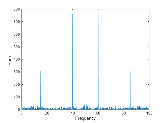
Create a signal with component frequencies at 15 Hz and 40 Hz, and inject random Gaussian noise.

rng('default')
fs = 100;                                % sample frequency (Hz)
t = 0:1/fs:10-1/fs;                      % 10 second span time vector
x = (1.3)*sin(2*pi*15*t) ...             % 15 Hz component
  + (1.7)*sin(2*pi*40*(t-2)) ...         % 40 Hz component
  + 2.5*randn(size(t));                  % Gaussian noise;

The Fourier transform of the signal identifies its frequency components. In MATLAB®, the fft function computes the Fourier transform using a fast Fourier transform algorithm. Use fft to compute the discrete Fourier transform of the signal.

Plot the power spectrum as a function of frequency. While noise disguises a signal’s frequency components in time-based space, the Fourier transform reveals them as spikes in power.

n = length(x);          % number of samples
f = (0:n-1)*(fs/n);     % frequency range
power = abs(y).^2/n;    % power of the DFT

plot(f,power)
xlabel('Frequency')
ylabel('Power')

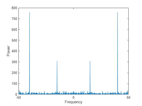
In many applications, it is more convenient to view the power spectrum centered at 0 frequency because it better represents the signal’s periodicity. Use the fftshift function to perform a circular shift on y, and plot the 0-centered power.

y0 = fftshift(y);         % shift y values
f0 = (-n/2:n/2-1)*(fs/n); % 0-centered frequency range
power0 = abs(y0).^2/n;    % 0-centered power

plot(f0,power0)
xlabel('Frequency')
ylabel('Power')

Audio Signal

You can use the Fourier transform to analyze the frequency spectrum of audio data.

The file bluewhale.au contains audio data from a Pacific blue whale vocalization recorded by underwater microphones off the coast of California. The file is from the library of animal vocalizations maintained by the Cornell University Bioacoustics Research Program.

Because blue whale calls are so low, they are barely audible to humans. The time scale in the data is compressed by a factor of 10 to raise the pitch and make the call more clearly audible. Read and plot the audio data. You can use the command sound(x,fs) to listen to the audio.

whaleFile = 'bluewhale.au';
[x,fs] = audioread(whaleFile);

plot(x)
xlabel('Sample Number')
ylabel('Amplitude')

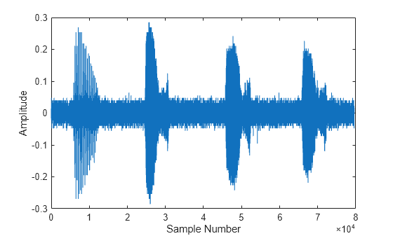
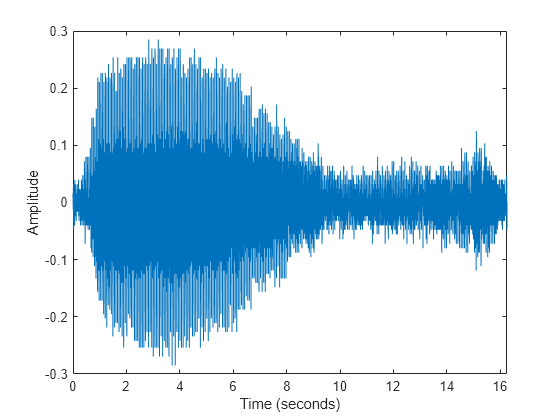
The first sound is a «trill» followed by three «moans». This example analyzes a single moan. Specify new data that approximately consists of the first moan, and correct the time data to account for the factor-of-10 speed-up. Plot the truncated signal as a function of time.

moan = x(2.45e4:3.10e4);
t = 10*(0:1/fs:(length(moan)-1)/fs);

plot(t,moan)
xlabel('Time (seconds)')
ylabel('Amplitude')
xlim([0 t(end)])

The Fourier transform of the data identifies frequency components of the audio signal. In some applications that process large amounts of data with fft, it is common to resize the input so that the number of samples is a power of 2. This can make the transform computation significantly faster, particularly for sample sizes with large prime factors. Specify a new signal length n that is a power of 2, and use the fft function to compute the discrete Fourier transform of the signal. fft automatically pads the original data with zeros to increase the sample size.

m = length(moan);       % original sample length
n = pow2(nextpow2(m));  % transform length
y = fft(moan,n);        % DFT of signal

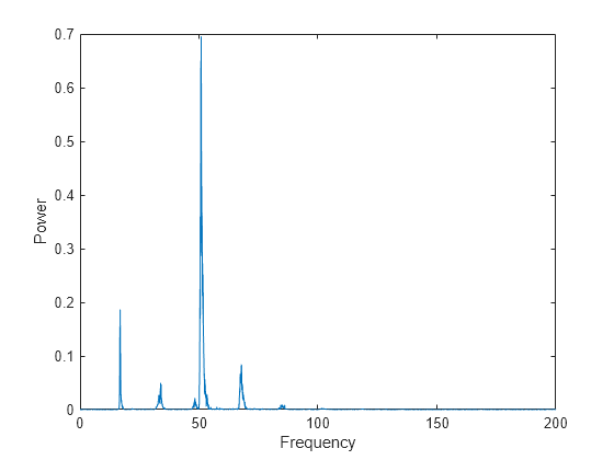
Adjust the frequency range due to the speed-up factor, and compute and plot the power spectrum of the signal. The plot indicates that the moan consists of a fundamental frequency around 17 Hz and a sequence of harmonics, where the second harmonic is emphasized.

f = (0:n-1)*(fs/n)/10;
power = abs(y).^2/n;      

plot(f(1:floor(n/2)),power(1:floor(n/2)))
xlabel('Frequency')
ylabel('Power')

Syntax

Description

example

s = spectrogram(x) returns the
Short-Time Fourier Transform
(STFT) of the input signal x. Each column of
s contains an estimate of the short-term,
time-localized frequency content of x. The magnitude
squared of s is known as the
spectrogram time-frequency representation of
x
[1].

example

s = spectrogram(x,window)
uses window to divide the signal into segments and perform
windowing.

example

s = spectrogram(x,window,noverlap)
uses noverlap samples of overlap between adjoining
segments.

example

s = spectrogram(x,window,noverlap,nfft)
uses nfft sampling points to calculate the discrete Fourier
transform.

example

[s,w,t] = spectrogram(___)
returns a vector of normalized frequencies, w, and a vector of time
instants, t, at which the STFT is
computed. This syntax can include any combination of input arguments from
previous syntaxes.

example

[s,f,t] = spectrogram(___,fs)
returns a vector of cyclical frequencies, f, expressed in terms of
the sample rate fs. fs must be the
fifth input to spectrogram. To input a sample rate and
still use the default values of the preceding optional arguments, specify these
arguments as empty, [].

example

[s,w,t] = spectrogram(x,window,noverlap,w)
returns the STFT at the normalized frequencies specified in w. w must
have at least two elements, because otherwise the function interprets it as
nfft.

example

[s,f,t] = spectrogram(x,window,noverlap,f,fs)
returns the STFT at the cyclical frequencies specified in f. f must
have at least two elements, because otherwise the function interprets it as
nfft.

example

[___,ps] = spectrogram(___,spectrumtype)
also returns a matrix, ps, proportional to the spectrogram
of x.

If you specify spectrumtype as
"psd", each column of ps
contains an estimate of the power spectral density (PSD) of a
windowed segment.
If you specify spectrumtype as
"power", each column of
ps contains an estimate of the power
spectrum of a windowed segment.

example

[___] = spectrogram(___,"reassigned") reassigns
each PSD or power spectrum estimate to the location of its center of energy. If
your signal contains well-localized temporal or spectral components, then this
option generates a sharper spectrogram.

example

[___,ps,fc,tc] = spectrogram(___)
also returns two matrices, fc and tc,
containing the frequency and time of the center of energy of each PSD or power
spectrum estimate.

example

[___] = spectrogram(___,freqrange)
returns the PSD or power spectrum estimate over the frequency range specified by
freqrange. Valid options for
freqrange are "onesided",
"twosided", and "centered".

example

[___] = spectrogram(___,Name=Value)
specifies additional options using name-value arguments. Options include the
minimum threshold and output time dimension.

example

spectrogram(___) with no output arguments plots
ps in decibels in the current figure window.

example

spectrogram(___,freqloc) specifies
the axis on which to plot the frequency.

Examples

collapse all

Default Values of Spectrogram

Generate Nx=1024 samples of a signal that consists of a sum of sinusoids. The normalized frequencies of the sinusoids are 2π/5 rad/sample and 4π/5 rad/sample. The higher frequency sinusoid has 10 times the amplitude of the other sinusoid.

N = 1024;
n = 0:N-1;

w0 = 2*pi/5;
x = sin(w0*n)+10*sin(2*w0*n);

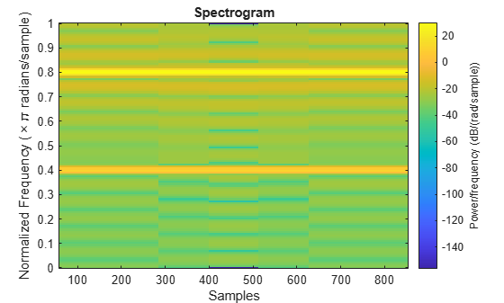
Compute the short-time Fourier transform using the function defaults. Plot the spectrogram.

s = spectrogram(x);

spectrogram(x,'yaxis')

Repeat the computation.

Divide the signal into sections of length nsc=⌊Nx/4.5⌋.
Window the sections using a Hamming window.
Specify 50% overlap between contiguous sections.
To compute the FFT, use max(256,2p) points, where p=⌈log2nsc⌉.

Verify that the two approaches give identical results.

Nx = length(x);
nsc = floor(Nx/4.5);
nov = floor(nsc/2);
nff = max(256,2^nextpow2(nsc));

t = spectrogram(x,hamming(nsc),nov,nff);

maxerr = max(abs(abs(t(:))-abs(s(:))))

Divide the signal into 8 sections of equal length, with 50% overlap between sections. Specify the same FFT length as in the preceding step. Compute the short-time Fourier transform and verify that it gives the same result as the previous two procedures.

ns = 8;
ov = 0.5;
lsc = floor(Nx/(ns-(ns-1)*ov));

t = spectrogram(x,lsc,floor(ov*lsc),nff);

maxerr = max(abs(abs(t(:))-abs(s(:))))

Compare `spectrogram` Function and STFT Definition

Generate a signal that consists of a complex-valued convex quadratic chirp sampled at 600 Hz for 2 seconds. The chirp has an initial frequency of 250 Hz and a final frequency of 50 Hz.

fs = 6e2;
ts = 0:1/fs:2;
x = chirp(ts,250,ts(end),50,"quadratic",0,"convex","complex");

spectrogram Function

Use the spectrogram function to compute the STFT of the signal.

Divide the signal into segments, each M=49 samples long.
Specify L=11 samples of overlap between adjoining segments.
Discard the final, shorter segment.
Window each segment with a Bartlett window.
Evaluate the discrete Fourier transform of each segment at NDFT=1024 points. By default, spectrogram computes two-sided transforms for complex-valued signals.

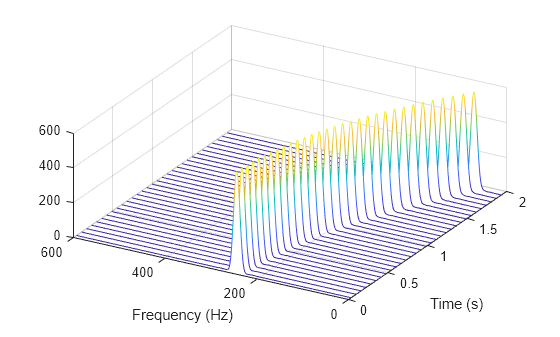
M = 49;
L = 11;
g = bartlett(M);
Ndft = 1024;

[s,f,t] = spectrogram(x,g,L,Ndft,fs);

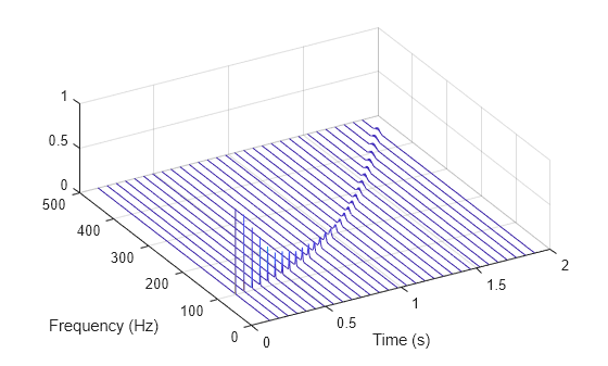
Use the waterplot function to compute and display the spectrogram, defined as the magnitude squared of the STFT.

STFT Definition

Compute the STFT of the Nx-sample signal using the definition. Divide the signal into ⌊Nx-LM-L⌋ overlapping segments. Window each segment and evaluate its discrete Fourier transform at NDFT points.

[segs,~] = buffer(1:length(x),M,L,"nodelay");

X = fft(x(segs).*g,Ndft);

Compute the time and frequency ranges for the STFT.

To find the time values, divide the time vector into overlapping segments. The time values are the midpoints of the segments, with each segment treated as an interval open at the lower end.
To find the frequency values, specify a Nyquist interval closed at zero frequency and open at the lower end.

tbuf = ts(segs);
tint = mean(tbuf(2:end,:));

fint = 0:fs/Ndft:fs-fs/Ndft;

Compare the output of spectrogram to the definition. Display the spectrogram.

maxdiff = max(max(abs(s-X)))

function waterplot(s,f,t)
% Waterfall plot of spectrogram
    waterfall(f,t,abs(s)'.^2)
    set(gca,XDir="reverse",View=[30 50])
    xlabel("Frequency (Hz)")
    ylabel("Time (s)")
end

Compare `spectrogram` and `stft` Functions

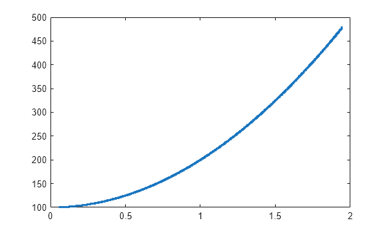
Generate a signal consisting of a chirp sampled at 1.4 kHz for 2 seconds. The frequency of the chirp decreases linearly from 600 Hz to 100 Hz during the measurement time.

fs = 1400;
x = chirp(0:1/fs:2,600,2,100);

stft Defaults

Compute the STFT of the signal using the spectrogram and stft functions. Use the default values of the stft function:

Divide the signal into 128-sample segments and window each segment with a periodic Hann window.
Specify 96 samples of overlap between adjoining segments. This length is equivalent to 75% of the window length.
Specify 128 DFT points and center the STFT at zero frequency, with the frequency expressed in hertz.

Verify that the two results are equal.

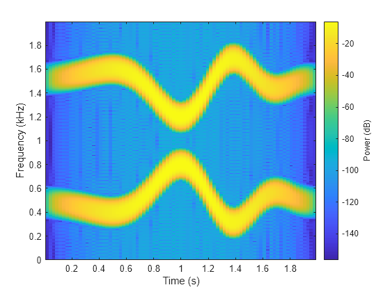
M = 128;
g = hann(M,"periodic");
L = 0.75*M;
Ndft = 128;

[sp,fp,tp] = spectrogram(x,g,L,Ndft,fs,"centered");

[s,f,t] = stft(x,fs);

dff = max(max(abs(sp-s)))

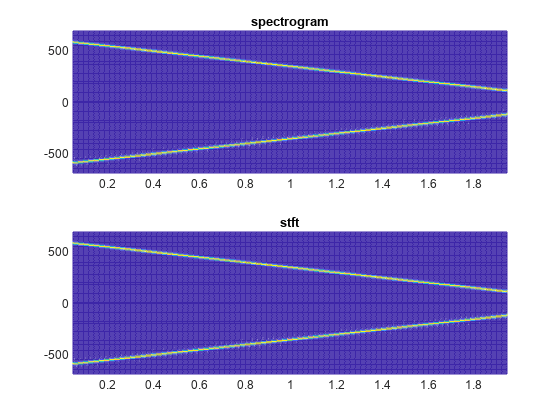
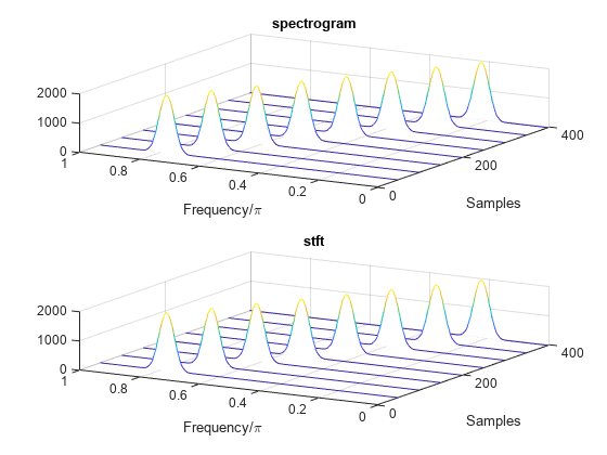
Use the mesh function to plot the two outputs.

nexttile
mesh(tp,fp,abs(sp).^2)
title("spectrogram")
view(2), axis tight

nexttile
mesh(t,f,abs(s).^2)
title("stft")
view(2), axis tight

spectrogram Defaults

Repeat the computation using the default values of the spectrogram function:

Divide the signal into segments of length M=⌊Nx/4.5⌋, where Nx is the length of the signal. Window each segment with a Hamming window.
Specify 50% overlap between segments.
To compute the FFT, use max(256,2⌈log2M⌉) points. Compute the spectrogram only for positive normalized frequencies.

M = floor(length(x)/4.5);
g = hamming(M);
L = floor(M/2);
Ndft = max(256,2^nextpow2(M));

[sx,fx,tx] = spectrogram(x);

[st,ft,tt] = stft(x,Window=g,OverlapLength=L, ...
    FFTLength=Ndft,FrequencyRange="onesided");

dff = max(max(sx-st))

Use the waterplot function to plot the two outputs. Divide the frequency axis by π in both cases. For the stft output, divide the sample numbers by the effective sample rate, 2π.

figure
nexttile
waterplot(sx,fx/pi,tx)
title("spectrogram")

nexttile
waterplot(st,ft/pi,tt/(2*pi))
title("stft")

function waterplot(s,f,t)
% Waterfall plot of spectrogram
    waterfall(f,t,abs(s)'.^2)
    set(gca,XDir="reverse",View=[30 50])
    xlabel("Frequency/pi")
    ylabel("Samples")
end

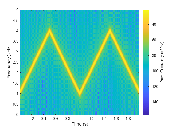
Spectrogram and Instantaneous Frequency

Use the spectrogram function to measure and track the instantaneous frequency of a signal.

Generate a quadratic chirp sampled at 1 kHz for two seconds. Specify the chirp so that its frequency is initially 100 Hz and increases to 200 Hz after one second.

fs = 1000;
t = 0:1/fs:2-1/fs;
y = chirp(t,100,1,200,'quadratic');

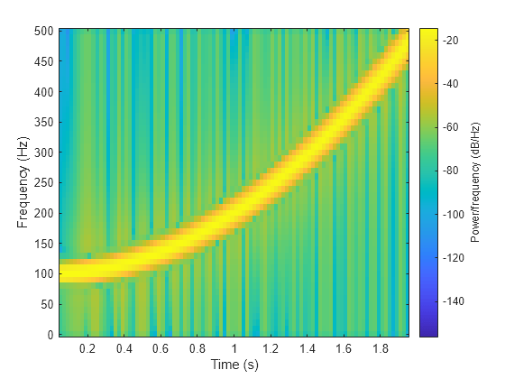
Estimate the spectrum of the chirp using the short-time Fourier transform implemented in the spectrogram function. Divide the signal into sections of length 100, windowed with a Hamming window. Specify 80 samples of overlap between adjoining sections and evaluate the spectrum at ⌊100/2+1⌋=51 frequencies.

spectrogram(y,100,80,100,fs,'yaxis')

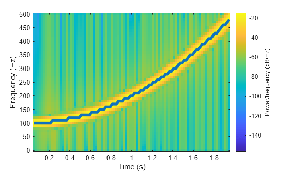
Track the chirp frequency by finding the time-frequency ridge with highest energy across the ⌊(2000-80)/(100-80)⌋=96 time points. Overlay the instantaneous frequency on the spectrogram plot.

[~,f,t,p] = spectrogram(y,100,80,100,fs);

[fridge,~,lr] = tfridge(p,f);

hold on
plot3(t,fridge,abs(p(lr)),'LineWidth',4)
hold off

Spectrogram of Complex Signal

Generate 512 samples of a chirp with sinusoidally varying frequency content.

N = 512;
n = 0:N-1;

x = exp(1j*pi*sin(8*n/N)*32);

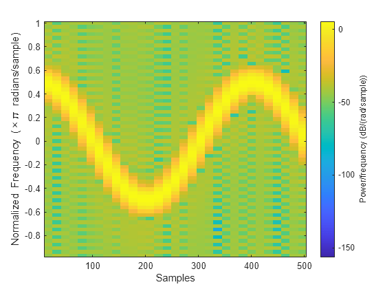
Compute the centered two-sided short-time Fourier transform of the chirp. Divide the signal into 32-sample segments with 16-sample overlap. Specify 64 DFT points. Plot the spectrogram.

[scalar,fs,ts] = spectrogram(x,32,16,64,'centered');

spectrogram(x,32,16,64,'centered','yaxis')

Obtain the same result by computing the spectrogram on 64 equispaced frequencies over the interval (-π,π]. The 'centered' option is not necessary.

fintv = -pi+pi/32:pi/32:pi;

[vector,fv,tv] = spectrogram(x,32,16,fintv);

spectrogram(x,32,16,fintv,'yaxis')

Compare `spectrogram` and `pspectrum` Functions

Generate a signal that consists of a voltage-controlled oscillator and three Gaussian atoms. The signal is sampled at fs=2 kHz for 2 seconds.

fs = 2000;
tx = 0:1/fs:2;
gaussFun = @(A,x,mu,f) exp(-(x-mu).^2/(2*0.03^2)).*sin(2*pi*f.*x)*A';
s = gaussFun([1 1 1],tx',[0.1 0.65 1],[2 6 2]*100)*1.5;
x = vco(chirp(tx+.1,0,tx(end),3).*exp(-2*(tx-1).^2),[0.1 0.4]*fs,fs);
x = s+x';

Short-Time Fourier Transforms

Use the pspectrum function to compute the STFT.

Divide the Nx-sample signal into segments of length M=80 samples, corresponding to a time resolution of 80/2000=40 milliseconds.
Specify L=16 samples or 20% of overlap between adjoining segments.
Window each segment with a Kaiser window and specify a leakage ℓ=0.7.

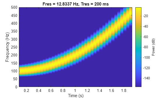
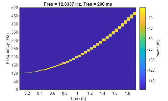
M = 80;
L = 16;
lk = 0.7;

[S,F,T] = pspectrum(x,fs,"spectrogram", ...
    TimeResolution=M/fs,OverlapPercent=L/M*100, ...
    Leakage=lk);

Compare to the result obtained with the spectrogram function.

Specify the window length and overlap directly in samples.
pspectrum always uses a Kaiser window as g(n). The leakage ℓ and the shape factor β of the window are related by β=40×(1-ℓ).
pspectrum always uses NDFT=1024 points when computing the discrete Fourier transform. You can specify this number if you want to compute the transform over a two-sided or centered frequency range. However, for one-sided transforms, which are the default for real signals, spectrogram uses 1024/2+1=513 points. Alternatively, you can specify the vector of frequencies at which you want to compute the transform, as in this example.
If a signal cannot be divided exactly into k=⌊Nx-LM-L⌋ segments, spectrogram truncates the signal whereas pspectrum pads the signal with zeros to create an extra segment. To make the outputs equivalent, remove the final segment and the final element of the time vector.
spectrogram returns the STFT, whose magnitude squared is the spectrogram. pspectrum returns the segment-by-segment power spectrum, which is already squared but is divided by a factor of ∑ng(n) before squaring.
For one-sided transforms, pspectrum adds an extra factor of 2 to the spectrogram.

g = kaiser(M,40*(1-lk));

k = (length(x)-L)/(M-L);
if k~=floor(k)
    S = S(:,1:floor(k));
    T = T(1:floor(k));
end

[s,f,t] = spectrogram(x/sum(g)*sqrt(2),g,L,F,fs);

Use the waterplot function to display the spectrograms computed by the two functions.

subplot(2,1,1)
waterplot(sqrt(S),F,T)
title("pspectrum")

subplot(2,1,2)
waterplot(s,f,t)
title("spectrogram")

maxd = max(max(abs(abs(s).^2-S)))

Power Spectra and Convenience Plots

The spectrogram function has a fourth argument that corresponds to the segment-by-segment power spectrum or power spectral density. Similar to the output of pspectrum, the ps argument is already squared and includes the normalization factor ∑ng(n). For one-sided spectrograms of real signals, you still have to include the extra factor of 2. Set the scaling argument of the function to "power".

[~,~,~,ps] = spectrogram(x*sqrt(2),g,L,F,fs,"power");

max(abs(S(:)-ps(:)))

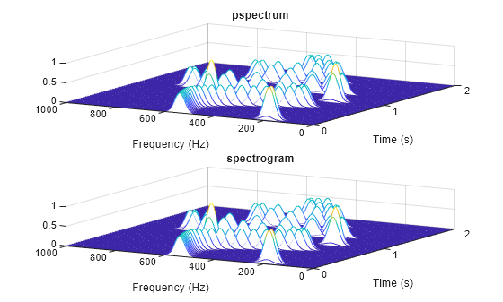
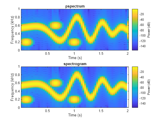
When called with no output arguments, both pspectrum and spectrogram plot the spectrogram of the signal in decibels. Include the factor of 2 for one-sided spectrograms. Set the colormaps to be the same for both plots. Set the x-limits to the same values to make visible the extra segment at the end of the pspectrum plot. In the spectrogram plot, display the frequency on the y-axis.

subplot(2,1,1)
pspectrum(x,fs,"spectrogram", ...
    TimeResolution=M/fs,OverlapPercent=L/M*100, ...
    Leakage=lk)
title("pspectrum")
cc = clim;
xl = xlim;

subplot(2,1,2)
spectrogram(x*sqrt(2),g,L,F,fs,"power","yaxis")
title("spectrogram")
clim(cc)
xlim(xl)

function waterplot(s,f,t)
% Waterfall plot of spectrogram
    waterfall(f,t,abs(s)'.^2)
    set(gca,XDir="reverse",View=[30 50])
    xlabel("Frequency (Hz)")
    ylabel("Time (s)")
end

Reassigned Spectrogram of Quadratic Chirp

Generate a chirp signal sampled for 2 seconds at 1 kHz. Specify the chirp so that its frequency is initially 100 Hz and increases to 200 Hz after 1 second.

fs = 1000;
t = 0:1/fs:2;
y = chirp(t,100,1,200,"quadratic");

Estimate the reassigned spectrogram of the signal.

Divide the signal into sections of length 128, windowed with a Kaiser window with shape parameter β=18.
Specify 120 samples of overlap between adjoining sections.
Evaluate the spectrum at ⌊128/2⌋=65 frequencies and ⌊(length(x)-120)/(128-120)⌋=235 time bins.

Use the spectrogram function with no output arguments to plot the reassigned spectrogram. Display frequency on the y-axis and time on the x-axis.

spectrogram(y,kaiser(128,18),120,128,fs, ...
    "reassigned","yaxis")

Redo the plot using the imagesc function. Specify the y-axis direction so that the frequency values increase from bottom to top. Add eps to the reassigned spectrogram to avoid potential negative infinities when converting to decibels.

[~,fr,tr,pxx] = spectrogram(y,kaiser(128,18),120,128,fs, ...
    "reassigned");

imagesc(tr,fr,pow2db(pxx+eps))
axis xy
xlabel("Time (s)")
ylabel("Frequency (Hz)")
colorbar

Spectrogram with Threshold

Generate a chirp signal sampled for 2 seconds at 1 kHz. Specify the chirp so that its frequency is initially 100 Hz and increases to 200 Hz after 1 second.

Fs = 1000;
t = 0:1/Fs:2;
y = chirp(t,100,1,200,'quadratic');

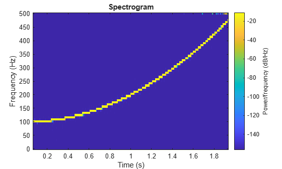
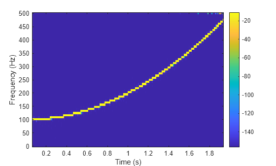
Estimate the time-dependent power spectral density (PSD) of the signal.

Divide the signal into sections of length 128, windowed with a Kaiser window with shape parameter β=18.
Specify 120 samples of overlap between adjoining sections.
Evaluate the spectrum at ⌊128/2⌋=65 frequencies and ⌊(length(x)-120)/(128-120)⌋=235 time bins.

Output the frequency and time of the center of gravity of each PSD estimate. Set to zero those elements of the PSD smaller than -30 dB.

[~,~,~,pxx,fc,tc] = spectrogram(y,kaiser(128,18),120,128,Fs, ...
    'MinThreshold',-30);

Plot the nonzero elements as functions of the center-of-gravity frequencies and times.

plot(tc(pxx>0),fc(pxx>0),'.')

Compute Centered and One-Sided Spectrograms

Generate a signal that consists of a real-valued chirp sampled at 2 kHz for 2 seconds.

fs = 2000;
tx = 0:1/fs:2;
x = vco(-chirp(tx,0,tx(end),2).*exp(-3*(tx-1).^2), ...
    [0.1 0.4]*fs,fs).*hann(length(tx))';

Two-Sided Spectrogram

Compute and plot the two-sided STFT of the signal.

Divide the signal into segments, each M=73 samples long.
Specify L=24 samples of overlap between adjoining segments.
Discard the final, shorter segment.
Window each segment with a flat-top window.
Evaluate the discrete Fourier transform of each segment at NDFT=895 points, noting that it is an odd number.

M = 73;
L = 24;
g = flattopwin(M);
Ndft = 895;
neven = ~mod(Ndft,2);

[stwo,f,t] = spectrogram(x,g,L,Ndft,fs,"twosided");

Use the spectrogram function with no output arguments to plot the two-sided spectrogram.

spectrogram(x,g,L,Ndft,fs,"twosided","power","yaxis");

Compute the two-sided spectrogram using the definition. Divide the signal into M-sample segments with L samples of overlap between adjoining segments. Window each segment and compute its discrete Fourier transform at NDFT points.

[segs,~] = buffer(1:length(x),M,L,"nodelay");

Xtwo = fft(x(segs).*g,Ndft);

Compute the time and frequency ranges.

To find the time values, divide the time vector into overlapping segments. The time values are the midpoints of the segments, with each segment treated as an interval open at the lower end.
To find the frequency values, specify a Nyquist interval closed at zero frequency and open at the upper end.

tbuf = tx(segs);
ttwo = mean(tbuf(2:end,:));

ftwo = 0:fs/Ndft:fs*(1-1/Ndft);

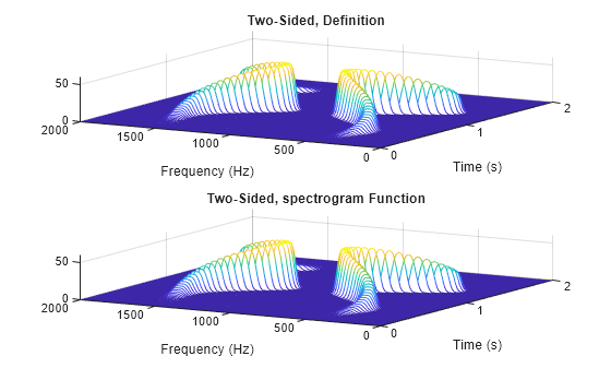
Compare the outputs of spectrogram to the definitions. Use the waterplot function to display the spectrograms.

diffs = [max(max(abs(stwo-Xtwo))) max(abs(f-ftwo')) max(abs(t-ttwo))]

diffs = 1×3
10^-12 ×

         0    0.2274    0.0002

figure
nexttile
waterplot(Xtwo,ftwo,ttwo)
title("Two-Sided, Definition")

nexttile
waterplot(stwo,f,t)
title("Two-Sided, spectrogram Function")

Centered Spectrogram

Compute the centered spectrogram of the signal.

Use the same time values that you used for the two-sided STFT.
Use the fftshift function to shift the zero-frequency component of the STFT to the center of the spectrum.
For odd-valued NDFT, the frequency interval is open at both ends. For even-valued NDFT, the frequency interval is open at the lower end and closed at the upper end.

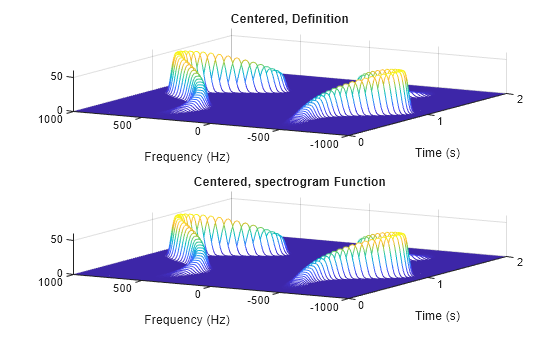
Compare the outputs and display the spectrograms.

tcen = ttwo;

if ~neven
    Xcen = fftshift(Xtwo,1);
    fcen = -fs/2*(1-1/Ndft):fs/Ndft:fs/2;
else
    Xcen = fftshift(circshift(Xtwo,-1),1);
    fcen = (-fs/2*(1-1/Ndft):fs/Ndft:fs/2)+fs/Ndft/2;
end

[scen,f,t] = spectrogram(x,g,L,Ndft,fs,"centered");

diffs = [max(max(abs(scen-Xcen))) max(abs(f-fcen')) max(abs(t-tcen))]

diffs = 1×3
10^-12 ×

         0    0.2274    0.0002

figure
nexttile
waterplot(Xcen,fcen,tcen)
title("Centered, Definition")

nexttile
waterplot(scen,f,t)
title("Centered, spectrogram Function")

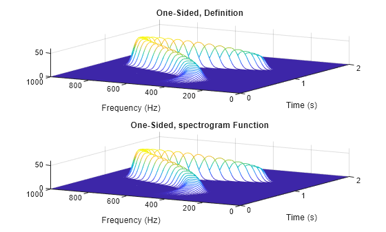
One-Sided Spectrogram

Compute the one-sided spectrogram of the signal.

Use the same time values that you used for the two-sided STFT.
For odd-valued NDFT, the one-sided STFT consists of the first (NDFT+1)/2 rows of the two-sided STFT. For even-valued NDFT, the one-sided STFT consists of the first NDFT/2+1 rows of the two-sided STFT.
For odd-valued NDFT, the frequency interval is closed at zero frequency and open at the Nyquist frequency. For even-valued NDFT, the frequency interval is closed at both ends.

Compare the outputs and display the spectrograms. For real-valued signals, the "onesided" argument is optional.

tone = ttwo;

if ~neven
    Xone = Xtwo(1:(Ndft+1)/2,:);
else
    Xone = Xtwo(1:Ndft/2+1,:);
end

fone = 0:fs/Ndft:fs/2;

[sone,f,t] = spectrogram(x,g,L,Ndft,fs);

diffs = [max(max(abs(sone-Xone))) max(abs(f-fone')) max(abs(t-tone))]

diffs = 1×3
10^-12 ×

         0    0.1137    0.0002

figure
nexttile
waterplot(Xone,fone,tone)
title("One-Sided, Definition")

nexttile
waterplot(sone,f,t)
title("One-Sided, spectrogram Function")

function waterplot(s,f,t)
% Waterfall plot of spectrogram
waterfall(f,t,abs(s)'.^2)
set(gca,XDir="reverse",View=[30 50])
xlabel("Frequency (Hz)")
ylabel("Time (s)")
end

Compute Segment PSDs and Power Spectra

The spectrogram function has a matrix containing either the power spectral density (PSD) or the power spectrum of each segment as the fourth output argument. The power spectrum is equal to the PSD multiplied by the equivalent noise bandwidth (ENBW) of the window.

Generate a signal that consists of a logarithmic chirp sampled at 1 kHz for 1 second. The chirp has an initial frequency of 400 Hz that decreases to 10 Hz by the end of the measurement.

fs = 1000;
tt = 0:1/fs:1-1/fs;
y = chirp(tt,400,tt(end),10,"logarithmic");

Segment PSDs and Power Spectra with Sample Rate

Divide the signal into 102-sample segments and window each segment with a Hann window. Specify 12 samples of overlap between adjoining segments and 1024 DFT points.

M = 102;
g = hann(M);
L = 12;
Ndft = 1024;

Compute the spectrogram of the signal with the default PSD spectrum type. Output the STFT and the array of segment power spectral densities.

[s,f,t,p] = spectrogram(y,g,L,Ndft,fs);

Repeat the computation with the spectrum type specified as "power". Output the STFT and the array of segment power spectra.

[r,~,~,q] = spectrogram(y,g,L,Ndft,fs,"power");

Verify that the spectrogram is the same in both cases. Plot the spectrogram using a logarithmic scale for the frequency.

max(max(abs(s).^2-abs(r).^2))

waterfall(f,t,abs(s)'.^2)
set(gca,XScale="log",...
    XDir="reverse",View=[30 50])

Verify that the power spectra are equal to the power spectral densities multiplied by the ENBW of the window.

max(max(abs(q-p*enbw(g,fs))))

Verify that the matrix of segment power spectra is proportional to the spectrogram. The proportionality factor is the square of the sum of the window elements.

max(max(abs(s).^2-q*sum(g)^2))

Segment PSDs and Power Spectra with Normalized Frequencies

Repeat the computation, but now work in normalized frequencies. The results are the same when you specify the sample rate as 2π.

[~,~,~,pn] = spectrogram(y,g,L,Ndft);
[~,~,~,qn] = spectrogram(y,g,L,Ndft,"power");

max(max(abs(qn-pn*enbw(g,2*pi))))

Track Chirps in Audio Signal

Load an audio signal that contains two decreasing chirps and a wideband splatter sound. Compute the short-time Fourier transform. Divide the waveform into 400-sample segments with 300-sample overlap. Plot the spectrogram.

load splat

% To hear, type soundsc(y,Fs)

sg = 400;
ov = 300;

spectrogram(y,sg,ov,[],Fs,"yaxis")
colormap bone

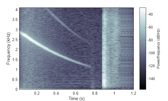
Use the spectrogram function to output the power spectral density (PSD) of the signal.

[s,f,t,p] = spectrogram(y,sg,ov,[],Fs);

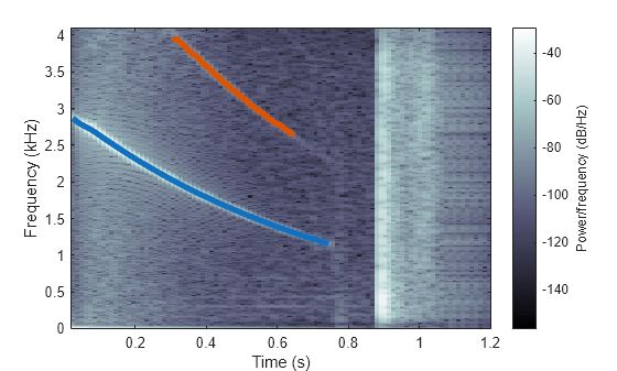
Track the two chirps using the medfreq function. To find the stronger, low-frequency chirp, restrict the search to frequencies above 100 Hz and to times before the start of the wideband sound.

f1 = f > 100;
t1 = t < 0.75;

m1 = medfreq(p(f1,t1),f(f1));

To find the faint high-frequency chirp, restrict the search to frequencies above 2500 Hz and to times between 0.3 seconds and 0.65 seconds.

f2 = f > 2500;
t2 = t > 0.3 & t < 0.65;

m2 = medfreq(p(f2,t2),f(f2));

Overlay the result on the spectrogram. Divide the frequency values by 1000 to express them in kHz.

hold on
plot(t(t1),m1/1000,LineWidth=4)
plot(t(t2),m2/1000,LineWidth=4)
hold off

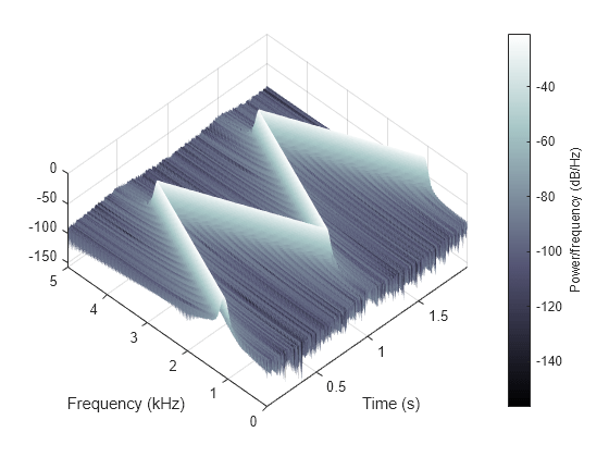
3D Spectrogram Visualization

Generate two seconds of a signal sampled at 10 kHz. Specify the instantaneous frequency of the signal as a triangular function of time.

fs = 10e3;
t = 0:1/fs:2;
x1 = vco(sawtooth(2*pi*t,0.5),[0.1 0.4]*fs,fs);

Compute and plot the spectrogram of the signal. Use a Kaiser window of length 256 and shape parameter β=5. Specify 220 samples of section-to-section overlap and 512 DFT points. Plot the frequency on the y-axis. Use the default colormap and view.

spectrogram(x1,kaiser(256,5),220,512,fs,'yaxis')

Change the view to display the spectrogram as a waterfall plot. Set the colormap to bone.

view(-45,65)
colormap bone

Input Arguments

collapse all

`x` — Input signal
vector

Input signal, specified as a row or column vector.

Example: cos(pi/4*(0:159))+randn(1,160) specifies a
sinusoid embedded in white Gaussian noise.

Data Types: single | double
Complex Number Support: Yes

`window` — Window
integer | vector | `[]`

Window, specified as an integer or as a row or column vector. Use
window to divide the signal into segments:

If window is an integer, then
spectrogram divides
x into segments of length
window and windows each segment with a
Hamming window of that length.
If window is a vector, then
spectrogram divides
x into segments of the same length as
the vector and windows each segment using
window.

If the length of x cannot be divided
exactly into an integer number of segments with
noverlap overlapping samples, then
x is truncated accordingly.

If you specify window as empty, then
spectrogram uses a Hamming window such that
x is divided into eight segments with
noverlap overlapping samples.

For a list of available windows, see Windows.

Example: hann(N+1) and
(1-cos(2*pi*(0:N)'/N))/2 both specify a Hann window
of length N + 1.

`noverlap` — Number of overlapped samples
positive integer | `[]`

Number of overlapped samples, specified as a positive integer.

If window is scalar, then
noverlap must be smaller than
window.
If window is a vector, then
noverlap must be smaller than the
length of window.

If you specify noverlap as empty, then
spectrogram uses a number that produces 50% overlap
between segments. If the segment length is unspecified, the function sets
noverlap to ⌊N_x/4.5⌋, where N_x is the
length of the input signal and the ⌊⌋ symbols denote the floor function.

`nfft` — Number of DFT points
positive integer scalar | `[]`

Number of DFT points, specified as a positive integer scalar. If you
specify nfft as empty, then
spectrogram sets the parameter to max(256,2^p), where p = ⌈log₂ N_w⌉, the ⌈⌉ symbols denote the ceiling function, and

N_w =
window if window
is a scalar.
N_w =
length(window)
if window is a vector.

`w` — Normalized frequencies
vector

Normalized frequencies, specified as a vector. w must
have at least two elements, because otherwise the function interprets it as
nfft. Normalized frequencies are in
rad/sample.

Example: pi./[2 4]

`f` — Cyclical frequencies
vector

Cyclical frequencies, specified as a vector. f must
have at least two elements, because otherwise the function interprets it as
nfft. The units of f are
specified by the sample rate, fs.

`fs` — Sample rate
1 Hz (default) | positive scalar

Sample rate, specified as a positive scalar. The sample rate is the number
of samples per unit time. If the unit of time is seconds, then the sample
rate is in Hz.

`freqrange` — Frequency range for PSD estimate
`"onesided"`
| `"twosided"` | `"centered"`

Frequency range for the PSD estimate, specified as
"onesided", "twosided", or
"centered". For real-valued signals, the default is
"onesided". For complex-valued signals, the default
is "twosided", and specifying
"onesided" results in an error.

"onesided" — returns the one-sided
spectrogram of a real input signal. If nfft is
even, then ps has nfft/2 +
1 rows and is computed over the interval [0, π] rad/sample. If nfft is odd,
then ps has (nfft + 1)/2
rows and the interval is [0, π) rad/sample. If you specify
fs, then the intervals are respectively [0,
fs/2] cycles/unit time and [0,
fs/2) cycles/unit time.
"twosided" — returns the two-sided
spectrogram of a real or complex-valued signal.
ps has nfft rows and
is computed over the interval [0, 2π) rad/sample. If you specify
fs, then the interval is [0,
fs) cycles/unit time.
"centered" — returns the centered
two-sided spectrogram of a real or complex-valued signal.
ps has nfft rows. If
nfft is even, then ps
is computed over the interval (–π,
π] rad/sample. If nfft is odd,
then ps is computed over (–π,
π) rad/sample. If you specify
fs, then the intervals are respectively
(–fs/2, fs/2]
cycles/unit time and (–fs/2,
fs/2) cycles/unit time.

`spectrumtype` — Power spectrum scaling
`"psd"` (default) | `"power"`

Power spectrum scaling, specified as "psd" or
"power".

Omitting spectrumtype, or specifying
"psd", returns the power spectral
density.
Specifying "power" scales each estimate of
the PSD by the equivalent noise bandwidth of the window. The
result is an estimate of the power at each frequency. If the
"reassigned" option is on, the function
integrates the PSD over the width of each frequency bin before
reassigning.

`freqloc` — Frequency display axis
`"xaxis"` (default) | `"yaxis"`

Frequency display axis, specified as "xaxis" or
"yaxis".

"xaxis" — displays frequency on the
x-axis and time on the
y-axis.
"yaxis" — displays frequency on the
y-axis and time on the
x-axis.

This argument is ignored if you call
spectrogram with output arguments.

Name-Value Arguments

Specify optional pairs of arguments as
Name1=Value1,...,NameN=ValueN, where Name is
the argument name and Value is the corresponding value.
Name-value arguments must appear after other arguments, but the order of the
pairs does not matter.

Example: spectrogram(x,100,OutputTimeDimension="downrows")
divides x into segments of length 100 and windows each segment
with a Hamming window of that length The output of the spectrogram has time
dimension down the rows.

Before R2021a, use commas to separate each name and value, and enclose
Name in quotes.

Example: spectrogram(x,100,'OutputTimeDimension','downrows')
divides x into segments of length 100 and windows each segment
with a Hamming window of that length The output of the spectrogram has time
dimension down the rows.

`MinThreshold` — Threshold
`-Inf` (default) | real scalar

Threshold, specified as a real scalar expressed in decibels.
spectrogram sets to zero those elements of
s such that
10 log₁₀(s) ≤ thresh.

`OutputTimeDimension` — Output time dimension
`"acrosscolumns"` (default) | `"downrows"`

Output time dimension, specified as "acrosscolumns"
or "downrows". Set this value to
"downrows", if you want the time dimension of
s, ps,
fc, and tc down the rows
and the frequency dimension along the columns. Set this value to
"acrosscolumns", if you want the time dimension
of s, ps,
fc, and tc across the
columns and frequency dimension along the rows. This input is ignored if
the function is called without output arguments.

Output Arguments

collapse all

`s` — Short-time Fourier transform
matrix

Short-time Fourier transform, returned as a matrix. Time increases across
the columns of s and frequency increases down the rows,
starting from zero.

If x is a signal of length
N_x, then
s has k columns, where
- k =
  ⌊(N_x –
  noverlap)/(window
  – noverlap)⌋ if
  window is a scalar.
- k =
  ⌊(N_x –
  noverlap)/(length(window)
  – noverlap)⌋ if
  window is a vector.
If x is real and
nfft is even, then
s has (nfft/2 + 1)
rows.
If x is real and
nfft is odd, then
s has (nfft + 1)/2
rows.
If x is complex-valued, then
s has nfft
rows.

Note

When freqrange is set to
"onesided", spectrogram
outputs the s values in the positive Nyquist
range and does not conserve the total power.

s is not affected by the
"reassigned" option.

`w` — Normalized frequencies
vector

Normalized frequencies, returned as a vector. w has a length equal to the
number of rows of s.

`t` — Time instants
vector

Time instants, returned as a vector. The time values in
t correspond to the midpoint of each
segment.

`f` — Cyclical frequencies
vector

Cyclical frequencies, returned as a vector. f has a length equal to the
number of rows of s.

`ps` — Power spectral density or power spectrum
matrix

Power spectral density (PSD) or power spectrum, returned as a matrix.

If x is real and
freqrange is left unspecified or set to
"onesided", then ps
contains the one-sided modified periodogram estimate of the PSD
or power spectrum of each segment. The function multiplies the
power by 2 at all frequencies except 0 and the Nyquist frequency
to conserve the total power.
If x is complex-valued or if
freqrange is set to
"twosided" or
"centered", then ps
contains the two-sided modified periodogram estimate of the PSD
or power spectrum of each segment.
If you specify a vector of normalized frequencies in w or a vector
of cyclical frequencies in f, then
ps contains the modified periodogram
estimate of the PSD or power spectrum of each segment evaluated
at the input frequencies.

`fc`, `tc` — Center-of-energy frequencies and times
matrices

Center-of-energy frequencies and times, returned as matrices of the same
size as the short-time Fourier transform. If you do not specify a sample
rate, then the elements of fc are returned as normalized
frequencies.

More About

collapse all

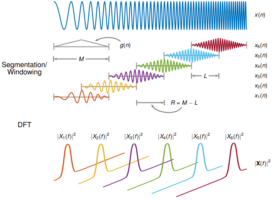
Short-Time Fourier Transform

The short-time Fourier transform (STFT) is used to analyze how the frequency
content of a nonstationary signal changes over time. The magnitude squared of the STFT is
known as the spectrogram time-frequency representation of the signal.
For more information about the spectrogram and how to compute it using Signal Processing Toolbox™ functions, see Spectrogram Computation with Signal Processing Toolbox.

The STFT of a signal is computed by sliding an analysis window
g(n) of length M over the signal and calculating the
discrete Fourier transform (DFT) of each segment of windowed data. The window hops over the
original signal at intervals of R samples, equivalent to L = M –
R samples of overlap between adjoining segments. Most window functions taper
off at the edges to avoid spectral ringing. The DFT of each windowed segment is added to a
complex-valued matrix that contains the magnitude and phase for each point in time and
frequency. The STFT matrix has

columns, where N_x is the length
of the signal x(n) and the ⌊⌋ symbols denote the floor function. The number of rows in the matrix equals N_DFT, the number of DFT points, for centered and two-sided transforms and an
odd number close to N_DFT/2 for one-sided transforms of real-valued signals.

The mth column of the STFT matrix X(f)=[X1(f)X2(f)X3(f)⋯Xk(f)] contains the DFT of the windowed data centered about time mR:

The short-time Fourier transform is invertible. The inversion process
overlap-adds the windowed segments to compensate for the signal attenuation at
the window edges. For more information, see Inverse Short-Time Fourier Transform.
The istft function inverts the STFT of a signal.
Under a specific set of circumstances it is possible to achieve «perfect
reconstruction» of a signal. For more information, see Perfect Reconstruction.
The stftmag2sig returns an estimate of a signal reconstructed from
the magnitude of its STFT.

Tips

If a short-time Fourier transform has zeros, its conversion
to decibels results in negative infinities that cannot be plotted.
To avoid this potential difficulty, spectrogram adds eps to
the short-time Fourier transform when you call it with no output arguments.

References

[1] Boashash, Boualem, ed.
Time Frequency Signal Analysis and Processing: A Comprehensive
Reference. Second edition. EURASIP and Academic Press Series in Signal
and Image Processing. Amsterdam and Boston: Academic Press, 2016.

[2] Chassande-Motin, Éric,
François Auger, and Patrick Flandrin. «Reassignment.» In Time-Frequency
Analysis: Concepts and Methods. Edited by Franz Hlawatsch and François
Auger. London: ISTE/John Wiley and Sons, 2008.

[3] Fulop, Sean A., and Kelly
Fitz. «Algorithms for computing the time-corrected instantaneous frequency (reassigned)
spectrogram, with applications.» Journal of the Acoustical Society of
America. Vol. 119, January 2006, pp. 360–371.

[4] Oppenheim, Alan V., and Ronald W. Schafer, with John R. Buck. Discrete-Time
Signal Processing. Second edition. Upper Saddle River, NJ: Prentice
Hall, 1999.

[5] Rabiner, Lawrence R., and Ronald W. Schafer. Digital
Processing of Speech Signals. Englewood Cliffs, NJ: Prentice-Hall,
1978.

Extended Capabilities

Tall Arrays
Calculate with arrays that have more rows than fit in memory.

Usage notes and limitations:

Input must be a tall column vector.
The window argument must always be specified.
OutputTimeDimension must be always specified and set
to "downrows".
The reassigned option is not supported.
Syntaxes with no output arguments are not supported.

For more information,
see Tall Arrays.

C/C++ Code Generation
Generate C and C++ code using MATLAB® Coder™.

Usage notes and limitations:

Arguments specified using name-value arguments must be compile-time
constants.
Variable sized window must be double
precision.

Thread-Based Environment
Run code in the background using MATLAB® `backgroundPool` or accelerate code with Parallel Computing Toolbox™ `ThreadPool`.

Usage notes and limitations:

The syntax with no output arguments is not supported.
The frequency vector must be uniformly spaced.

For more information, see Run MATLAB Functions in Thread-Based Environment.

GPU Arrays
Accelerate code by running on a graphics processing unit (GPU) using Parallel Computing Toolbox™.

This function fully supports GPU arrays. For more information, see Run MATLAB Functions on a GPU (Parallel Computing Toolbox).

Version History

Introduced before R2006a

expand all

R2023a: Visualize function outputs using Create Plot
Live Editor task

You can now use the Create
Plot Live Editor task to visualize the output of
spectrogram interactively. You can select different chart
types and set optional parameters. The task also automatically generates code that
becomes part of your live script.

pspectrum

Analyze signals in the frequency and time-frequency domains

Syntax

Description

example

p = pspectrum(x)
returns the power spectrum of x.

If x is a vector or a timetable with a vector
of data, then it is treated as a single channel.
If x is a matrix, a timetable with a matrix
variable, or a timetable with multiple vector variables, then the
spectrum is computed independently for each channel and stored in a
separate column of p.

example

p = pspectrum(x,fs)
returns the power spectrum of a vector or matrix signal sampled at a rate
fs.

example

p = pspectrum(x,t)
returns the power spectrum of a vector or matrix signal sampled at the time
instants specified in t.

example

p = pspectrum(___,type)
specifies the kind of spectral analysis performed by the function. Specify
type as 'power',
'spectrogram', or 'persistence'. This
syntax can include any combination of input arguments from previous
syntaxes.

example

p = pspectrum(___,Name,Value)
specifies additional options using name-value pair arguments. Options include
the frequency resolution bandwidth and the percent overlap between adjoining
segments.

example

[p,f] = pspectrum(___)
returns the frequencies corresponding to the spectral estimates contained in
p.

example

[p,f,t] = pspectrum(___,'spectrogram')
also returns a vector of time instants corresponding to the centers of the
windowed segments used to compute short-time power spectrum estimates.

[p,f,pwr] = pspectrum(___,'persistence')
also returns a vector of power values corresponding to the estimates contained
in a persistence spectrum.

example

pspectrum(___) with no output arguments plots
the spectral estimate in the current figure window. For the plot, the function
converts p to dB using 10
log₁₀(p).

Examples

collapse all

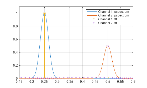
Power Spectra of Sinusoids

Generate 128 samples of a two-channel complex sinusoid.

The first channel has unit amplitude and a normalized sinusoid frequency of π/4 rad/sample
The second channel has an amplitude of 1/2 and a normalized frequency of π/2 rad/sample.

Compute and plot the power spectrum of each channel. Zoom in on the frequency range from 0.15π rad/sample to 0.6π rad/sample. pspectrum scales the spectrum so that, if the frequency content of a signal falls exactly within a bin, its amplitude in that bin is the true average power of the signal. For a complex exponential, the average power is the square of the amplitude. Verify by computing the discrete Fourier transform of the signal. For more details, see Measure Power of Deterministic Periodic Signals.

N = 128;
x = [1 1/sqrt(2)].*exp(1j*pi./[4;2]*(0:N-1)).';

[p,f] = pspectrum(x);

plot(f/pi,p)
hold on
stem(0:2/N:2-1/N,abs(fft(x)/N).^2)
hold off
axis([0.15 0.6 0 1.1])
legend("Channel "+[1;2]+", "+["pspectrum" "fft"])
grid

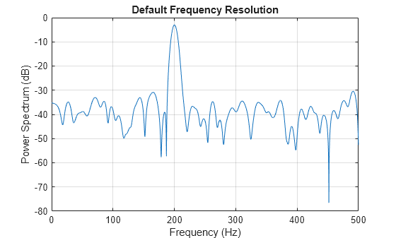
Generate a sinusoidal signal sampled at 1 kHz for 296 milliseconds and embedded in white Gaussian noise. Specify a sinusoid frequency of 200 Hz and a noise variance of 0.1². Store the signal and its time information in a MATLAB® timetable.

Fs = 1000;
t = (0:1/Fs:0.296)';
x = cos(2*pi*t*200)+0.1*randn(size(t));
xTable = timetable(seconds(t),x);

Compute the power spectrum of the signal. Express the spectrum in decibels and plot it.

[pxx,f] = pspectrum(xTable);

plot(f,pow2db(pxx))
grid on
xlabel('Frequency (Hz)')
ylabel('Power Spectrum (dB)')
title('Default Frequency Resolution')

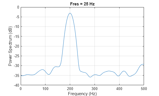
Recompute the power spectrum of the sinusoid, but now use a coarser frequency resolution of 25 Hz. Plot the spectrum using the pspectrum function with no output arguments.

pspectrum(xTable,'FrequencyResolution',25)

Two-Sided Spectra

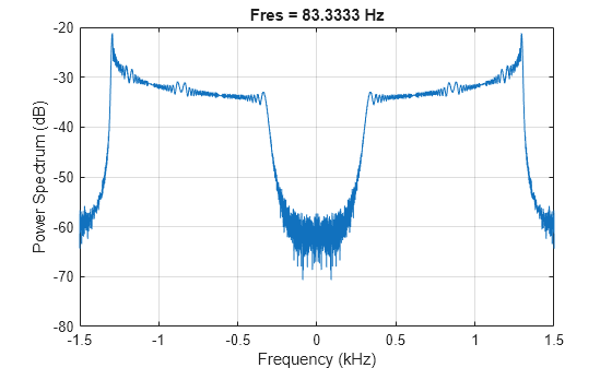
Generate a signal sampled at 3 kHz for 1 second. The signal is a convex quadratic chirp whose frequency increases from 300 Hz to 1300 Hz during the measurement. The chirp is embedded in white Gaussian noise.

fs = 3000;
t = 0:1/fs:1-1/fs;

x1 = chirp(t,300,t(end),1300,'quadratic',0,'convex') + ...
    randn(size(t))/100;

Compute and plot the two-sided power spectrum of the signal using a rectangular window. For real signals, pspectrum plots a one-sided spectrum by default. To plot a two-sided spectrum, set TwoSided to true.

pspectrum(x1,fs,'Leakage',1,'TwoSided',true)

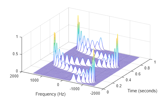
Generate a complex-valued signal with the same duration and sample rate. The signal is a chirp with sinusoidally varying frequency content and embedded in white noise. Compute the spectrogram of the signal and display it as a waterfall plot. For complex-valued signals, the spectrogram is two-sided by default.

x2 = exp(2j*pi*100*cos(2*pi*2*t)) + randn(size(t))/100;

[p,f,t] = pspectrum(x2,fs,'spectrogram');

waterfall(f,t,p')
xlabel('Frequency (Hz)')
ylabel('Time (seconds)')
wtf = gca;
wtf.XDir = 'reverse';
view([30 45])

Window Leakage and Tone Resolution

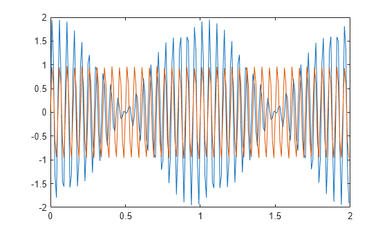
Generate a two-channel signal sampled at 100 Hz for 2 seconds.

The first channel consists of a 20 Hz tone and a 21 Hz tone. Both tones have unit amplitude.
The second channel also has two tones. One tone has unit amplitude and a frequency of 20 Hz. The other tone has an amplitude of 1/100 and a frequency of 30 Hz.

fs = 100;
t = (0:1/fs:2-1/fs)';

x = sin(2*pi*[20 20].*t) + [1 1/100].*sin(2*pi*[21 30].*t);

Embed the signal in white noise. Specify a signal-to-noise ratio of 40 dB. Plot the signals.

x = x + randn(size(x)).*std(x)/db2mag(40);

plot(t,x)

Compute the spectra of the two channels and display them.

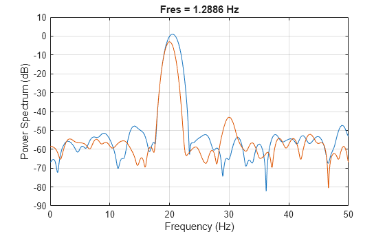
The default value for the spectral leakage, 0.5, corresponds to a resolution bandwidth of about 1.29 Hz. The two tones in the first channel are not resolved. The 30 Hz tone in the second channel is visible, despite being much weaker than the other one.

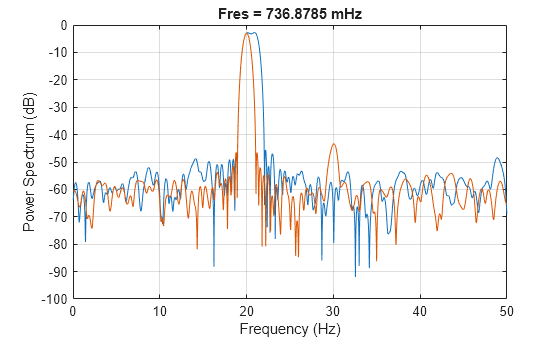
Increase the leakage to 0.85, equivalent to a resolution of about 0.74 Hz. The weak tone in the second channel is clearly visible.

pspectrum(x,t,'Leakage',0.85)

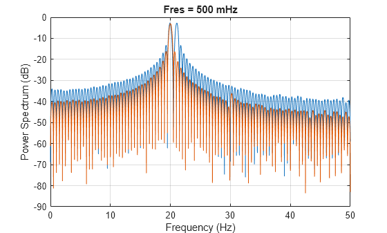
Increase the leakage to the maximum value. The resolution bandwidth is approximately 0.5 Hz. The two tones in the first channel are resolved. The weak tone in the second channel is masked by the large window sidelobes.

pspectrum(x,t,'Leakage',1)

Compare `spectrogram` and `pspectrum` Functions

Generate a signal that consists of a voltage-controlled oscillator and three Gaussian atoms. The signal is sampled at fs=2 kHz for 2 seconds.

fs = 2000;
tx = 0:1/fs:2;
gaussFun = @(A,x,mu,f) exp(-(x-mu).^2/(2*0.03^2)).*sin(2*pi*f.*x)*A';
s = gaussFun([1 1 1],tx',[0.1 0.65 1],[2 6 2]*100)*1.5;
x = vco(chirp(tx+.1,0,tx(end),3).*exp(-2*(tx-1).^2),[0.1 0.4]*fs,fs);
x = s+x';

Short-Time Fourier Transforms

Use the pspectrum function to compute the STFT.

Divide the Nx-sample signal into segments of length M=80 samples, corresponding to a time resolution of 80/2000=40 milliseconds.
Specify L=16 samples or 20% of overlap between adjoining segments.
Window each segment with a Kaiser window and specify a leakage ℓ=0.7.

M = 80;
L = 16;
lk = 0.7;

[S,F,T] = pspectrum(x,fs,"spectrogram", ...
    TimeResolution=M/fs,OverlapPercent=L/M*100, ...
    Leakage=lk);

Compare to the result obtained with the spectrogram function.

Specify the window length and overlap directly in samples.
pspectrum always uses a Kaiser window as g(n). The leakage ℓ and the shape factor β of the window are related by β=40×(1-ℓ).
pspectrum always uses NDFT=1024 points when computing the discrete Fourier transform. You can specify this number if you want to compute the transform over a two-sided or centered frequency range. However, for one-sided transforms, which are the default for real signals, spectrogram uses 1024/2+1=513 points. Alternatively, you can specify the vector of frequencies at which you want to compute the transform, as in this example.
If a signal cannot be divided exactly into k=⌊Nx-LM-L⌋ segments, spectrogram truncates the signal whereas pspectrum pads the signal with zeros to create an extra segment. To make the outputs equivalent, remove the final segment and the final element of the time vector.
spectrogram returns the STFT, whose magnitude squared is the spectrogram. pspectrum returns the segment-by-segment power spectrum, which is already squared but is divided by a factor of ∑ng(n) before squaring.
For one-sided transforms, pspectrum adds an extra factor of 2 to the spectrogram.

g = kaiser(M,40*(1-lk));

k = (length(x)-L)/(M-L);
if k~=floor(k)
    S = S(:,1:floor(k));
    T = T(1:floor(k));
end

[s,f,t] = spectrogram(x/sum(g)*sqrt(2),g,L,F,fs);

Use the waterplot function to display the spectrograms computed by the two functions.

subplot(2,1,1)
waterplot(sqrt(S),F,T)
title("pspectrum")

subplot(2,1,2)
waterplot(s,f,t)
title("spectrogram")

maxd = max(max(abs(abs(s).^2-S)))

Power Spectra and Convenience Plots

[~,~,~,ps] = spectrogram(x*sqrt(2),g,L,F,fs,"power");

max(abs(S(:)-ps(:)))

subplot(2,1,1)
pspectrum(x,fs,"spectrogram", ...
    TimeResolution=M/fs,OverlapPercent=L/M*100, ...
    Leakage=lk)
title("pspectrum")
cc = clim;
xl = xlim;

subplot(2,1,2)
spectrogram(x*sqrt(2),g,L,F,fs,"power","yaxis")
title("spectrogram")
clim(cc)
xlim(xl)

function waterplot(s,f,t)
% Waterfall plot of spectrogram
    waterfall(f,t,abs(s)'.^2)
    set(gca,XDir="reverse",View=[30 50])
    xlabel("Frequency (Hz)")
    ylabel("Time (s)")
end

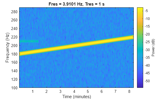
Persistence Spectrum of Transient Signal

Visualize an interference narrowband signal embedded within a broadband signal.

Generate a chirp sampled at 1 kHz for 500 seconds. The frequency of the chirp increases from 180 Hz to 220 Hz during the measurement.

fs = 1000;
t = (0:1/fs:500)';

x = chirp(t,180,t(end),220) + 0.15*randn(size(t));

The signal also contains a 210 Hz sinusoid. The sinusoid has an amplitude of 0.05 and is present only for 1/6 of the total signal duration.

idx = floor(length(x)/6);
x(1:idx) = x(1:idx) + 0.05*cos(2*pi*t(1:idx)*210);

Compute the spectrogram of the signal. Restrict the frequency range from 100 Hz to 290 Hz. Specify a time resolution of 1 second. Both signal components are visible.

pspectrum(x,fs,'spectrogram', ...
    'FrequencyLimits',[100 290],'TimeResolution',1)

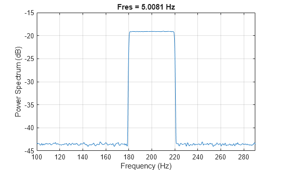
Compute the power spectrum of the signal. The weak sinusoid is obscured by the chirp.

pspectrum(x,fs,'FrequencyLimits',[100 290])

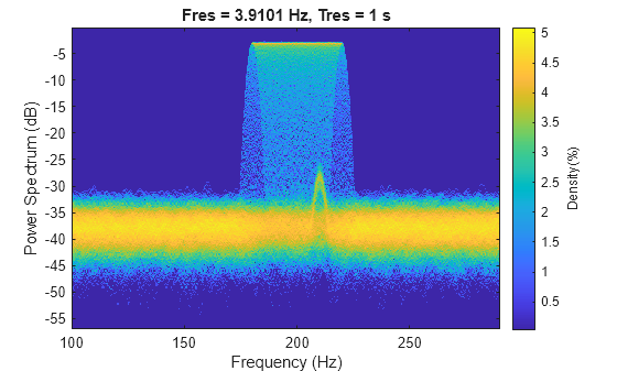
Compute the persistence spectrum of the signal. Now both signal components are clearly visible.

pspectrum(x,fs,'persistence', ...
    'FrequencyLimits',[100 290],'TimeResolution',1)

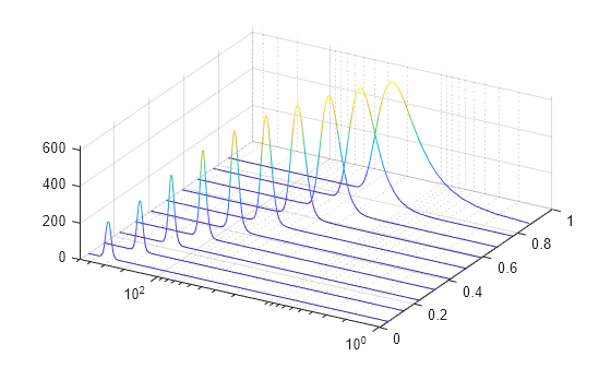
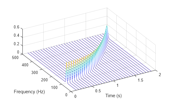
Spectrogram and Reassigned Spectrogram of Chirp

Generate a quadratic chirp sampled at 1 kHz for 2 seconds. The chirp has an initial frequency of 100 Hz that increases to 200 Hz at t = 1 second. Compute the spectrogram using the default settings of the pspectrum function. Use the waterfall function to plot the spectrogram.

fs = 1e3;
t = 0:1/fs:2;
y = chirp(t,100,1,200,"quadratic");

[sp,fp,tp] = pspectrum(y,fs,"spectrogram");

waterfall(fp,tp,sp')
set(gca,XDir="reverse",View=[60 60])
ylabel("Time (s)")
xlabel("Frequency (Hz)")

Compute and display the reassigned spectrogram.

[sr,fr,tr] = pspectrum(y,fs,"spectrogram",Reassign=true);

waterfall(fr,tr,sr')
set(gca,XDir="reverse",View=[60 60])
ylabel("Time (s)")
xlabel("Frequency (Hz)")

Recompute the spectrogram using a time resolution of 0.2 second. Visualize the result using the pspectrum function with no output arguments.

pspectrum(y,fs,"spectrogram",TimeResolution=0.2)

Compute the reassigned spectrogram using the same time resolution.

pspectrum(y,fs,"spectrogram",TimeResolution=0.2,Reassign=true)

Spectrogram of Dial Tone Signal

Create a signal, sampled at 4 kHz, that resembles pressing all the keys of a digital telephone. Save the signal as a MATLAB® timetable.

fs = 4e3;
t = 0:1/fs:0.5-1/fs;

ver = [697 770 852 941];
hor = [1209 1336 1477];

tones = [];

for k = 1:length(ver)
    for l = 1:length(hor)
        tone = sum(sin(2*pi*[ver(k);hor(l)].*t))';
        tones = [tones;tone;zeros(size(tone))];
    end
end

% To hear, type soundsc(tones,fs)

S = timetable(seconds(0:length(tones)-1)'/fs,tones);

Compute the spectrogram of the signal. Specify a time resolution of 0.5 second and zero overlap between adjoining segments. Specify the leakage as 0.85, which is approximately equivalent to windowing the data with a Hann window.

pspectrum(S,'spectrogram', ...
    'TimeResolution',0.5,'OverlapPercent',0,'Leakage',0.85)

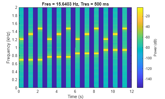
The spectrogram shows that each key is pressed for half a second, with half-second silent pauses between keys. The first tone has a frequency content concentrated around 697 Hz and 1209 Hz, corresponding to the digit '1' in the DTMF standard.

Input Arguments

collapse all

`x` — Input signal
vector | matrix | timetable

Input signal, specified as a vector, a matrix, or a MATLAB^®
timetable.

If x is a timetable, then it must contain
increasing finite row times.
If x is a timetable representing a
multichannel signal, then it must have either a single variable
containing a matrix or multiple variables consisting of
vectors.

If x is nonuniformly sampled, then
pspectrum interpolates the signal to a uniform grid
to compute spectral estimates. The function uses linear interpolation and
assumes a sample time equal to the median of the differences between
adjacent time points. For a nonuniformly sampled signal to be supported, the
median time interval and the mean time interval must obey

Example: cos(pi./[4;2]*(0:159))'+randn(160,2) is a
two-channel signal consisting of sinusoids embedded in white
noise.

Example: timetable(seconds(0:4)',rand(5,2)) specifies a
two-channel random variable sampled at 1 Hz for 4 seconds.

Example: timetable(seconds(0:4)',rand(5,1),rand(5,1))
specifies a two-channel random variable sampled at 1 Hz for 4
seconds.

Data Types: single | double
Complex Number Support: Yes

`fs` — Sample rate
2π (default) | positive numeric scalar

Sample rate, specified as a positive numeric scalar.

`t` — Time values
vector | `datetime` array | `duration` array | `duration` scalar

Time values, specified as a vector, a datetime or duration array, or a
duration scalar representing the time interval
between samples.

Example: seconds(0:1/100:1) is a
duration array representing
1 second of sampling at 100 Hz.

Example: seconds(1) is a
duration scalar representing
a 1-second time difference between consecutive signal
samples.

`type` — Type of spectrum to compute
`'power'` (default) | `'spectrogram'` | `'persistence'`

Type of spectrum to compute, specified as 'power',
'spectrogram', or 'persistence':

'power' — Compute the power spectrum of the
input. Use this option to analyze the frequency content of a
stationary signal. For more information, Spectrum Computation.
'spectrogram' — Compute the spectrogram of
the input. Use this option to analyze how the frequency content
of a signal changes over time. For more information, see Spectrogram Computation.
'persistence' — Compute the persistence
power spectrum of the input. Use this option to visualize the
fraction of time that a particular frequency component is
present in a signal. For more information, see Persistence Spectrum Computation.

Note

The 'spectrogram' and
'persistence' options do not support multichannel
input.

Name-Value Arguments

Before R2021a, use commas to separate each name and value, and enclose
Name in quotes.

Example: 'Leakage',1,'Reassign',true,'MinThreshold',-35 windows
the data using a rectangular window, computes a reassigned spectrum estimate, and
sets all values smaller than –35 dB to zero.

`FrequencyLimits` — Frequency band limits
`[0 fs/2]` (default) | two-element numeric vector

Frequency band limits, specified as the comma-separated pair
consisting of 'FrequencyLimits' and a two-element
numeric vector:

If the input contains time information, then the frequency
band is expressed in Hz.
If the input does not contain time information, then the
frequency band is expressed in normalized units of
rad/sample.

By default, pspectrum computes the spectrum over
the whole Nyquist range:

If the specified frequency band contains a region that
falls outside the Nyquist range, then
pspectrum truncates the frequency
band.
If the specified frequency band lies completely outside of
the Nyquist range, then pspectrum
throws an error.

See Spectrum Computation
for more information about the Nyquist range.

If x is nonuniformly sampled, then
pspectrum linearly interpolates the signal to a
uniform grid and defines an effective sample rate equal to the inverse
of the median of the differences between adjacent time points. Express
'FrequencyLimits' in terms of the effective
sample rate.

Example: [0.2*pi 0.7*pi] computes the spectrum of a
signal with no time information from
0.2π to
0.7π
rad/sample.

`FrequencyResolution` — Frequency resolution bandwidth
real numeric scalar

Frequency resolution bandwidth, specified as the comma-separated pair
consisting of 'FrequencyResolution' and a real
numeric scalar, expressed in Hz if the input contains time information,
or in normalized units of rad/sample if not. This argument cannot be
specified simultaneously with 'TimeResolution'. The
default value of this argument depends on the size of the input data.
See Spectrogram Computation
for details.

Example: pi/100 computes the spectrum of a signal
with no time information with a frequency resolution of
π/100
rad/sample.

`Leakage` — Spectral leakage
`0.5` (default) | real numeric scalar between 0 and 1

Spectral leakage, specified as the comma-separated pair consisting of
'Leakage' and a real numeric scalar between 0 and
1. 'Leakage' controls the Kaiser window sidelobe
attenuation relative to the mainlobe width, compromising between
improving resolution and decreasing leakage:

A large leakage value resolves closely spaced tones, but
masks nearby weak tones.
A small leakage value finds small tones in the vicinity of
larger tones, but smears close frequencies together.

Example: 'Leakage',0 reduces leakage to a minimum at
the expense of spectral resolution.

Example: 'Leakage',0.85 approximates windowing the
data with a Hann window.

Example: 'Leakage',1 is equivalent to windowing the
data with a rectangular window, maximizing leakage but improving
spectral resolution.

`MinThreshold` — Lower bound for nonzero values
`-Inf` (default) | real scalar

Lower bound for nonzero values, specified as the comma-separated pair
consisting of 'MinThreshold' and a real scalar.
pspectrum implements
'MinThreshold' differently based on the value
of the type argument:

'power' or
'spectrogram' —
pspectrum sets those elements of
p such that 10
log₁₀(p)
≤ 'MinThreshold' to zero. Specify
'MinThreshold' in decibels.
'persistence' —
pspectrum sets those elements of
p smaller than
'MinThreshold' to zero. Specify
'MinThreshold' between 0 and
100%.

`NumPowerBins` — Number of power bins for persistence spectrum
`256` (default) | integer between 20 and 1024

Number of power bins for persistence spectrum, specified as the
comma-separated pair consisting of 'NumPowerBins' and
an integer between 20 and 1024.

`OverlapPercent` — Overlap between adjoining segments
real scalar in the interval [0, 100)

Overlap between adjoining segments for spectrogram or persistence
spectrum, specified as the comma-separated pair consisting of
'OverlapPercent' and a real scalar in the
interval [0, 100). The default value of this argument depends on the
spectral window. See Spectrogram Computation
for details.

`Reassign` — Reassignment option
`false` (default) | `true`

Reassignment option, specified as the comma-separated pair consisting
of 'Reassign' and a logical value. If this option is
set to true, then pspectrum
sharpens the localization of spectral estimates by performing time and
frequency reassignment. The reassignment technique produces periodograms
and spectrograms that are easier to read and interpret. This technique
reassigns each spectral estimate to the center of energy of its bin
instead of the bin’s geometric center. The technique provides exact
localization for chirps and impulses.

`TimeResolution` — Time resolution of spectrogram or persistence spectrum
real scalar

Time resolution of spectrogram or persistence spectrum, specified as
the comma-separated pair consisting of
'TimeResolution' and a real scalar, expressed in
seconds if the input contains time information, or as an integer number
of samples if not. This argument controls the duration of the segments
used to compute the short-time power spectra that form spectrogram or
persistence spectrum estimates. 'TimeResolution'
cannot be specified simultaneously with
'FrequencyResolution'. The default value of
this argument depends on the size of the input data and, if it was
specified, the frequency resolution. See Spectrogram Computation
for details.

`TwoSided` — Two-sided spectral estimate
false | true

Two-sided spectral estimate, specified as the comma-separated pair
consisting of 'TwoSided' and a logical value.

If this option is true, the function
computes centered, two-sided spectrum estimates over [–π,
π]. If the input has time information, the
estimates are computed over [–f_s/2,
f_s/2], where
f_s is the
effective sample rate.
If this option is false, the function
computes one-sided spectrum estimates over the Nyquist range [0, π]. If the input has time information, the
estimates are computed over [0,
f_s/2], where
f_s is the
effective sample rate. To conserve the total power, the
function multiplies the power by 2 at all frequencies except
0 and the Nyquist frequency. This option is valid only for
real signals.

If not specified, 'TwoSided'
defaults to false for real input signals and to
true for complex input signals.

Output Arguments

collapse all

`p` — Spectrum
vector | matrix

Spectrum, returned as a vector or a matrix. The type and size of the
spectrum depends on the value of the type argument:

'power' — p contains
the power spectrum estimate of each channel of
x. In this case, p
is of size
N_f × N_ch,
where N_f is the length
of f and
N_ch is the number
of channels of x.
pspectrum scales the spectrum so that,
if the frequency content of a signal falls exactly within a bin,
its amplitude in that bin is the true average power of the
signal. For example, the average power of a sinusoid is one-half
the square of the sinusoid amplitude. For more details, see
Measure Power of Deterministic Periodic Signals.
'spectrogram' — p
contains an estimate of the short-term, time-localized power
spectrum of x. In this case,
p is of size
N_f × N_t,
where N_f is the length
of f and
N_t is the length
of t.
'persistence' — p
contains, expressed as percentages, the probabilities that the
signal has components of a given power level at a given time and
frequency location. In this case, p is of
size
N_pwr × N_f,
where N_pwr is the
length of pwr and
N_f is the length
of f.

`f` — Spectrum frequencies
vector

Spectrum frequencies, returned as a vector. If the input signal contains
time information, then f contains frequencies expressed
in Hz. If the input signal does not contain time information, then the
frequencies are in normalized units of rad/sample.

`t` — Time values of spectrogram
vector | `datetime` array | `duration` array

Time values of spectrogram, returned as a vector of time values in seconds
or a duration array. If the input does not have time
information, then t contains sample numbers. t contains the time values corresponding to the centers of
the data segments used to compute short-time power spectrum estimates.

If the input to pspectrum is a timetable,
then t has the same format as the time values of the
input timetable.
If the input to pspectrum is a numeric
vector sampled at a set of time instants specified by a numeric,
duration, or
datetime array,
then t has the same type and format as the input time
values.
If the input to pspectrum is a numeric
vector with a specified time difference between consecutive
samples, then t is a duration
array.

`pwr` — Power values of persistence spectrum
vector

Power values of persistence spectrum, returned as a vector.

More About

collapse all

Spectrum Computation

To compute signal spectra, pspectrum finds a
compromise between the spectral resolution achievable with the entire length of the
signal and the performance limitations that result from computing large FFTs:

If possible, the function computes a single modified periodogram of
the whole signal using a Kaiser window.
If it is not possible to compute a single modified periodogram in a
reasonable amount of time, the function computes a Welch periodogram: It
divides the signal into overlapping segments, windows each segment using
a Kaiser window, and averages the periodograms of the segments.

Spectral Windowing

Any real-world signal is measurable only for a finite length of time. This fact
introduces nonnegligible effects into Fourier analysis, which assumes that signals
are either periodic or infinitely long. Spectral windowing,
which assigns different weights to different signal samples, deals systematically
with finite-size effects.

The simplest way to window a signal is to assume that it is identically zero
outside of the measurement interval and that all samples are equally significant.
This «rectangular window» has discontinuous jumps at both ends that result in
spectral ringing. All other spectral windows taper at both ends to lessen this
effect by assigning smaller weights to samples close to the signal edges.

The windowing process always involves a compromise between conflicting aims:
improving resolution and decreasing leakage:

Resolution is the ability to know precisely how
the signal energy is distributed in the frequency space. A spectrum
analyzer with ideal resolution can distinguish two different tones (pure
sinusoids) present in the signal, no matter how close in frequency.
Quantitatively, this ability relates to the mainlobe width of the
transform of the window.
Leakage is the fact that, in a finite signal,
every frequency component projects energy content throughout the
complete frequency span. The amount of leakage in a spectrum can be
measured by the ability to detect a weak tone from noise in the presence
of a neighboring strong tone. Quantitatively, this ability relates to
the sidelobe level of the frequency transform of the window.
The spectrum is normalized so that a pure tone within that bandwidth,
if perfectly centered, has the correct amplitude.

The better the resolution, the higher the leakage, and vice versa. At
one end of the range, a rectangular window has the narrowest possible mainlobe and
the highest sidelobes. This window can resolve closely spaced tones if they have
similar energy content, but it fails to find the weaker one if they do not. At the
other end, a window with high sidelobe suppression has a wide mainlobe in which
close frequencies are smeared together.

pspectrum uses Kaiser windows to carry out windowing. For
Kaiser windows, the fraction of the signal energy captured by the mainlobe depends
most importantly on an adjustable shape factor,
β. pspectrum uses shape factors ranging
from β = 0, which corresponds to a rectangular window, to β = 40, where a wide mainlobe captures essentially all the spectral
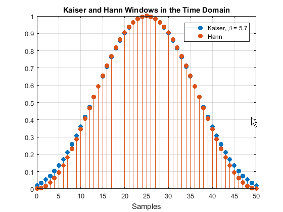
energy representable in double precision. An intermediate value of β ≈ 6 approximates a Hann window quite closely. To control
β, use the 'Leakage' name-value pair. If
you set 'Leakage' to ℓ, then
ℓ and β are related by β = 40(1 – ℓ). See kaiser for more
details.


51-point Hann window and 51-point Kaiser window with β = 5.7 in the time domain	51-point Hann window and 51-point Kaiser window with β = 5.7 in the frequency domain

Parameter and Algorithm Selection

To compute signal spectra, pspectrum initially determines the
resolution bandwidth, which measures how close two tones
can be and still be resolved. The resolution bandwidth has a theoretical value of

t_max – t_min, the record length, is the
time-domain duration of the selected signal region.
ENBW is the equivalent noise
bandwidth of the spectral window. See enbw for more
details.

Use the 'Leakage' name-value pair to control the
ENBW. The minimum value of the argument corresponds to a Kaiser window
with β = 40. The maximum value corresponds to a Kaiser window with β = 0.

In practice, however, pspectrum might lower the resolution.
Lowering the resolution makes it possible to compute the spectrum in a reasonable
amount of time and to display it with a finite number of pixels. For these practical
reasons, the lowest resolution bandwidth pspectrum can use is

where f_span is the width of the frequency band specified using
'FrequencyLimits'. If
'FrequencyLimits' is not specified, then
pspectrum uses the sample rate as f_span. RBW_performance cannot be adjusted.

To compute the spectrum of a signal, the function chooses the larger of the two
values, called the target resolution bandwidth:

If the resolution bandwidth is RBW_theory, then pspectrum computes a single
modified periodogram for the whole signal. The
function uses a Kaiser window with shape factor controlled by the
'Leakage' name-value pair. See periodogram for more
details.
If the resolution bandwidth is RBW_performance, then pspectrum computes a
Welch periodogram for the signal. The function:
1. Divides the signals into overlapping segments.
2. Windows each segment separately using a Kaiser window with the
  specified shape factor.
3. Averages the periodograms of all the segments.
Welch’s procedure is designed to reduce the variance of the
spectrum estimate by averaging different “realizations” of the
signals, given by the overlapping sections, and using the window to remove
redundant data. See pwelch for more details.
- The length of each segment (or, equivalently, of the window)
  is computed using
  
  where f_Nyquist is the Nyquist
  frequency. (If there is no aliasing, the Nyquist
  frequency is one-half the effective sample rate, defined as the
  inverse of the median of the differences between adjacent time
  points. The Nyquist range is [0,
  f_Nyquist] for real signals and [–f_Nyquist,
  f_Nyquist] for complex signals.)
- The stride length is found by adjusting an initial estimate,
  
  so that the first window starts exactly on
  the first sample of the first segment and the last window ends
  exactly on the last sample of the last segment.

Spectrogram Computation

To compute the time-dependent spectrum of a nonstationary signal,
pspectrum divides the signal into overlapping segments,
windows each segment with a Kaiser window, computes the short-time Fourier
transform, and then concatenates the transforms to form a matrix. For more
information, see Spectrogram Computation with Signal Processing Toolbox.

A nonstationary signal is a signal whose frequency content changes with time. The
spectrogram of a nonstationary signal is an estimate of
the time evolution of its frequency content. To construct the spectrogram of a
nonstationary signal, pspectrum follows these steps:

Divide the signal into equal-length segments. The segments must be
short enough that the frequency content of the signal does not change
appreciably within a segment. The segments may or may not
overlap.
Window each segment and compute its spectrum to get the
short-time Fourier transform.
Use the segment spectra to construct the spectrogram:
- If called with output arguments, concatenate the spectra
  to form a matrix.
- If called with no output arguments, display the power of
  each spectrum in decibels segment by segment. Depict the
  magnitudes side-by-side as an image with magnitude-dependent
  colormap.

The function can compute the spectrogram only for single-channel
signals.

Divide Signal into Segments

To construct a spectrogram, first divide the signal into possibly overlapping
segments. With the pspectrum function, you can control the
length of the segments and the amount of overlap between adjoining segments using
the 'TimeResolution' and 'OverlapPercent'
name-value pair arguments. If you do not specify the length and overlap, the
function chooses a length based on the entire length of the signal and an overlap
percentage given by

where ENBW is the equivalent noise bandwidth of the
spectral window. See enbw and Spectrum Computation for more
information.

Specified Time Resolution

If the signal does not have time information, specify the time resolution
(segment length) in samples. The time resolution must be an integer greater
than or equal to 1 and smaller than or equal to the signal length.

If the signal has time information, specify the time resolution in
seconds. The function converts the result into a number of samples and
rounds it to the nearest integer that is less than or equal to the number
but not smaller than 1. The time resolution must be smaller than or equal to
the signal duration.
Specify the overlap as a percentage of the segment length. The function
converts the result into a number of samples and rounds it to the nearest
integer that is less than or equal to the number.

Default Time Resolution

If you do not specify a time resolution, then pspectrum uses
the length of the entire signal to choose the length of the segments. The function
sets the time resolution as ⌈N/d⌉ samples, where the ⌈⌉ symbols denote the ceiling function, N is the
length of the signal, and d is a divisor that depends on
N:

Signal Length (N)	Divisor (d)	Segment Length
`2` samples – `63` samples	`2`	`1` sample – `32` samples
`64` samples – `255` samples	`8`	`8` samples – `32` samples
`256` samples – `2047` samples	`8`	`32` samples – `256` samples
`2048` samples – `4095` samples	`16`	`128` samples – `256` samples
`4096` samples – `8191` samples	`32`	`128` samples – `256` samples
`8192` samples – `16383` samples	`64`	`128` samples – `256` samples
`16384` samples – N samples	`128`	`128` samples – ⌈N / `128`⌉ samples

You can still specify the overlap between adjoining segments.
Specifying the overlap changes the number of segments. Segments that extend beyond
the signal endpoint are zero-padded.

Consider the seven-sample signal [s0 s1 s2 s3 s4 s5 s6].
Because ⌈7/2⌉ = ⌈3.5⌉ = 4, the function divides the signal into two segments of length four
when there is no overlap. The number of segments changes as the overlap
increases.

Number of Overlapping Samples	Resulting Segments
`0`	s0 s1 s2 s3 s4 s5 s6 0
`1`	s0 s1 s2 s3 s3 s4 s5 s6
`2`	s0 s1 s2 s3 s2 s3 s4 s5 s4 s5 s6 0
`3`	s0 s1 s2 s3 s1 s2 s3 s4 s2 s3 s4 s5 s3 s4 s5 s6

pspectrum zero-pads the signal if the last
segment extends beyond the signal endpoint. The function returns t, a
vector of time instants corresponding to the centers of the segments.

Window the Segments and Compute Spectra

After pspectrum divides the signal into overlapping segments,
the function windows each segment with a Kaiser window. The shape factor
β of the window, and therefore the leakage, can be adjusted
using the 'Leakage' name-value pair. The function then computes
the spectrum of each segment and concatenates the spectra to form the spectrogram
matrix. To compute the segment spectra, pspectrum follows the
procedure described in Spectrum Computation, except that
the lower limit of the resolution bandwidth is

Display Spectrum Power

If called with no output arguments, the function displays the power of the
short-time Fourier transform in decibels, using a color bar with the default
MATLAB colormap. The color bar comprises the full power range of the
spectrogram.

Persistence Spectrum Computation

The persistence spectrum is a
time-frequency view that shows the percentage of the time that a given frequency is
present in a signal. The persistence spectrum is a histogram in power-frequency
space. The longer a particular frequency persists in a signal as the signal evolves,
the higher its time percentage and thus the brighter or «hotter» its color in the
display. Use the persistence spectrum to identify signals hidden in other
signals.

To compute the persistence spectrum, pspectrum performs these steps:

Compute the spectrogram using the specified leakage, time resolution,
and overlap. See Spectrogram Computation
for more details.
Partition the power and frequency values into 2-D bins. (Use the
'NumPowerBins' name-value pair to specify the
number of power bins.)
For each time value, compute a bivariate histogram of the logarithm of
the power spectrum. For every power-frequency bin where there is signal
energy at that instant, increase the corresponding matrix element by 1.
Sum the histograms for all the time values.
Plot the accumulated histogram against the power and the frequency,
with the color proportional to the logarithm of the histogram counts
expressed as normalized percentages. To represent zero values, use
one-half of the smallest possible magnitude.

Power Spectra

Histograms

Accumulated
Histogram

References

[1] harris, fredric j. “On the Use of Windows for Harmonic Analysis with the
Discrete Fourier Transform.” Proceedings of the IEEE^®. Vol. 66, January 1978, pp. 51–83.

[2] Welch, Peter D. «The Use of Fast Fourier Transform for the Estimation of Power
Spectra: A Method Based on Time Averaging Over Short, Modified Periodograms.»
IEEE Transactions on Audio and Electroacoustics. Vol. 15, June
1967, pp. 70–73.

Extended Capabilities

C/C++ Code Generation
Generate C and C++ code using MATLAB® Coder™.

Usage notes and limitations:

Timetables are not supported for code generation.

GPU Arrays
Accelerate code by running on a graphics processing unit (GPU) using Parallel Computing Toolbox™.

Usage notes and limitations:

Persistence spectrum is not supported.
Reassigned spectrum or spectrogram is not supported.

For more information, see Run MATLAB Functions on a GPU (Parallel Computing Toolbox).

Version History

Introduced in R2017b

expand all

R2023a: Visualize function outputs using Create Plot Live Editor task

You can now use the Create
Plot Live Editor task to visualize the output of
pspectrum interactively. You can select different chart
types and set optional parameters. The task also automatically generates code that
becomes part of your live script.

Источник

Время на прочтение
7 мин

Количество просмотров 213K

По работе неоднократно сталкивался с необходимостью быстро определить наличие в сигнале гармонических составляющих. Часто для примерной оценки достаточно воспользоваться алгоритмом быстрого преобразования Фурье. Тем более, что его реализации есть практически во всех математических пакетах и библиотеках, да и собственноручно реализовать не составит особого труда. Между тем, опыт показывает, что, при всей своей простоте, метод начинает вызывать некоторые вопросы, когда возникает необходимость не просто посмотреть наличие дискреток в сигнале, но и выяснить их абсолютные значения, т.е. нормализовать полученный результат.

В этой статье я постараюсь объяснить, что же все-таки выдает в качестве результата fft (Fast Fourier transform) на примере MATLAB (и в качестве бонуса проведу небольшой ликбез по этому весьма полезному, на мой взгляд, языку).

MATLAB позволяет не заморачиваться с ручным удалением ненужных объектов, однако, при работе с более менее объемными массивами данных, имеет привычку капризничать и жаловаться на недостаток памяти. Для освобождения памяти используется процедура clear с указанием имени объекта, который необходимо удалить.

С этого и начнем. Так как все необходимое мы сгенерируем самостоятельно, можно смело удалять все, что накопилось в рабочем пространстве за активную сессию, просто добавив ключевое слово all:

clear all% Очистка памяти

Итак, прежде всего, зададим исходные данные для нашей модели. Фурье анализ идеально подходит для выделения гармонических сигналов на фоне помех. Для того чтобы продемонстрировать это, возьмем в качестве сигнала сумму некоторой постоянной и двух синусоид с разной частотой и амплитудой. Дисперсию шума возьмем в 3 раза больше амплитуды первой синусоиды. Так же зададим количество частотных полос, которые должен будет посчитать fft алгоритм. Точка с запятой в конце строк не обязательна, и если ее не ставить, результат вычисления функций и задания переменных будет дублироваться в командную строку, что можно использовать для отладки кода (однако, 512 значений сплошным полотном в командной строке вряд ли помогут вам, тем более что их вывод тоже занимает некоторое количество времени, так что все же лучше не забывать закрывать строки).

%% Параметры Tm=5;% Длина сигнала (с) Fd=512;% Частота дискретизации (Гц) Ak=0.5;% Постоянная составляющая (Попугаев) A1=1;% Амплитуда первой синусоиды (Попугаев) A2=0.7;% Амплитуда второй синусоиды (Попугаев) F1=13;% Частота первой синусоиды (Гц) F2=42;% Частота второй синусоиды (Гц) Phi1=0;% Начальная фаза первой синусоиды (Градусов) Phi2=37;% Начальная фаза второй синусоиды (Градусов) An=3*A1;% Дисперсия шума (Попугаев) FftL=1024;% Количество линий Фурье спектра

MATLAB (Matrix Laboratory), как следует из названия, предназначен прежде всего для работы с массивами, практически все алгоритмы счета в нем оптимизированы для работы с векторами. Обилие удобных инструментов работы так же ненавязчиво подталкивает представлять как можно больше исходных данных в виде матриц. В частности, можно легко сгенерировать массив возрастающих (убывающих) величин с заданным шагом (1Fd в данном примере):

%% Генерация рабочих массивов T=0:1/Fd:Tm;% Массив отсчетов времени

Случайный Гауссов шум задается функцией randn, результатом которой является массив размерности, заданной в ее параметрах. Для единообразия зададим его в виде строки (первый параметр 1) длиной соответствующей длине нашего массива отсчетов времен, что в свою очередь вычислим функцией length.

Noise=An*randn(1,length(T));% Массив случайного шума длиной равной массиву времени

Символ * используется для обозначения перемножения. Т.к. чаще всего действия производятся над векторами, то и умножение подразумевается векторное, но так же легко можно, не перегружая этот оператор, использовать его для поэлементного перемножения, добавив перед ним точку (.*). При умножении вектора на скаляр точка перед умножением не является обязательной. Также добавленная точка сделает поэлементным возведение в степень и деление.

Signal=Ak+A1*sind((F1*360).*T+Phi1)+A2*sind((F2*360).*T+Phi2);% Массив сигнала (смесь 2х синусоид и постоянной составляющей)

Теперь перейдем к тому, ради чего и затевалась данная статья — функции fft(). Аргументами стандартной функции MATLAB являются сам сигнал (в нашем случае Signal), размерность вектора-результата (FftL), а также измерение.
Последний аргумент определяет вдоль какого измерения располагается сигнал в случае если на вход подается многомерный массив (Иногда этот параметр ошибочно принимают за размерность преобразования Фурье, но это не так. Хотя в MATLAB есть реализации 2-хмерного fft2() и многомерного fftn() алгоритмов). Так как наш сигнал представляет собой вектор, то его вполне можно опустить.
Рассмотрим сначала сигнал без примеси шума. В качестве результата мы получим вектор комплексных чисел. Это и есть представление нашего сигнала в частотном домене в показательной форме. Т.е. модули этих комплексных чисел представляют амплитуды соответствующих частот (точнее полосы частот см. дальше), а аргументы – их начальные фазы. И если полученная фаза, однозначно вычисляется в радианах, то с амплитудой и частотами не все так просто.
Например, если мы просто применим к нашему сигналу преобразование Фурье, и возьмем абсолютные значения вектора на выходе, то получим приблизительно следующую картинку:

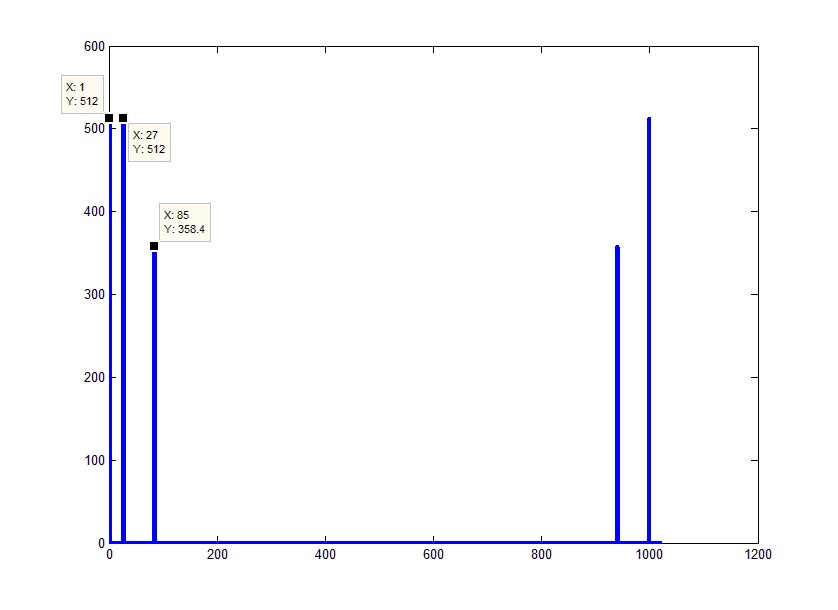
Для построения двухмерных графиков удобно использовать функцию plot. Основные параметры, используемые в этой функции – одномерные массивы точек, первый задает ось ординат, второй – значение функции в соответствующих точках. Если передать только один массив, то он будет отображен с фиксированным шагом 1.
Если присмотреться к полученной картинке выяснится, что она несколько отличается от наших ожиданий. На приведенном графике 5 пиков вместо ожидаемых 3х (постоянная + 2 синусоиды), их амплитуды не совпадают с амплитудами исходных сигналов, и ось абсцисс вряд ли отображает частоты.

Прежде всего, следует учитывать, что счет алгоритма устроен таким образом, что перебираются не только положительные, но и отрицательные частоты и правая часть графика является «зеркальным» отображением реального спектра. Т.е. на самом деле 0 (которому соответствует постоянная часть сигнала) должен приходиться на середину массива. Ситуацию можно поправить, совершив циклический сдвиг на половину длины массива. Для этих целей, в MATLAB существует функция сдвига fftshift(), смещающая первый элемент в середину массива:

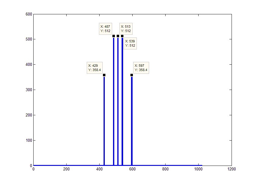
Теперь обратим внимание на ось значений.
Согласно теореме отсчетов (так же известной как теорема Найквиста-Шеннона или более патриотично теорема Котельникова) спектр дискретного сигнала будет ограничен половиной частоты дискретизации (Fd). Или в нашем случае –Fd/2 слева и Fd/2 справа. Т.е. весь полученный массив покрывает Fd частот. Отсюда, учитывая что мы знаем (вернее даже самостоятельно задали в качестве параметра) длину массива, получим частоты в виде массива значений от –Fd/2 до Fd/2 с шагом Fd/FftL (на самом деле крайняя правая частота будет меньше границы на один отсчет т.е. Fd/2-Fd/FftL):

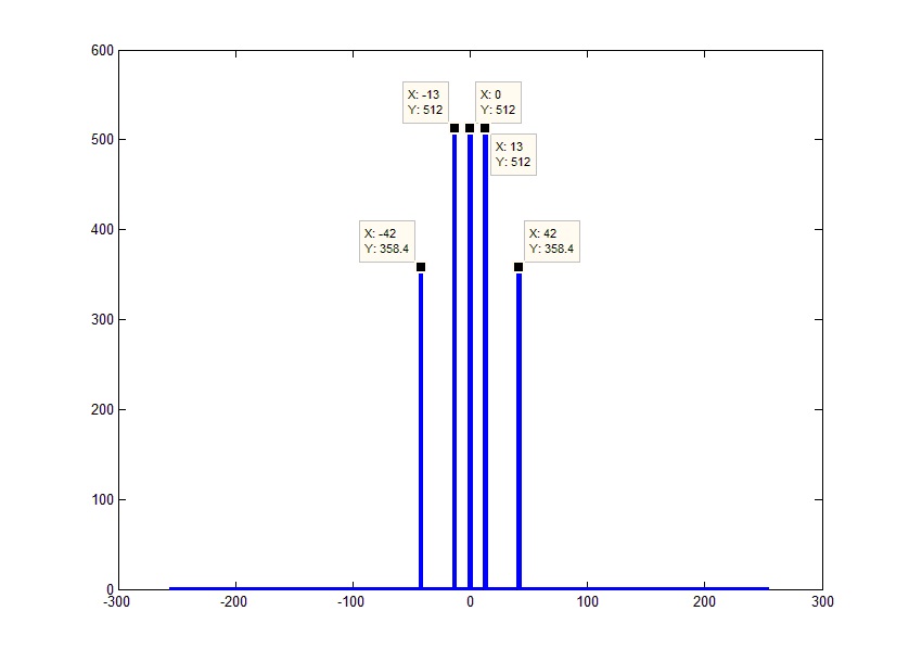
Если посмотреть на фазы частот, можно заметить, что они равны отрицательным фазам соответствующих отрицательных частот. Учитывая равенство амплитуд левой и правой частей спектра и соответствие их фаз с точностью до знака, весь спектр будет эквивалентен своей положительной части с удвоенной амплитудой. Исключение составляет только 0 элемент, который не имеет зеркальной половины. Таким образом, можно избавиться от «непонятных» и зачастую ненужных отрицательных частот. Это можно было сделать сразу просто отбросив конец исходного массива и помножив оставшиеся элементы на 2 (за исключением постоянной составляющей):

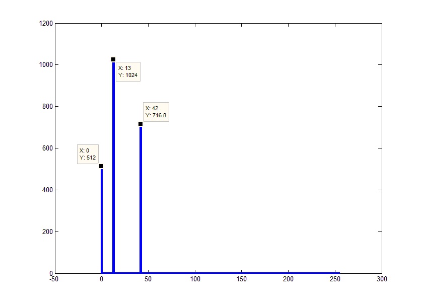
Теперь это уже похоже на тот результат, который мы ожидаем. Единственное, что смущает теперь – это амплитуды. С этим все достаточно просто. Т.к. быстрое преобразование Фурье фактически представляет собой суммирование сигнала перемноженного на ядро преобразования (комплексную экспоненту) для каждой из частот, то реальный результат будет меньше полученного ровно в количество суммирований (частот в результате), т.е. полученный результат надо разделить на количество элементов в результате (не забываем, что под результатом понимается весь ответ, вместе с отброшенной частью, т.е. наше заданное FftL):

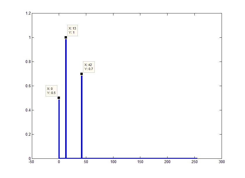
Стоит упомянуть еще одну вещь. В спектральном представлении вычисляется не значение сигнала на той частоте на которую попал алгоритм (как мы помним частоты следуют с шагом Fd/FftL), а значение в полосе (шириной равной шагу). Т.е. если в эту полосу попало несколько дискреток, то они суммируются. Для примера можно уменьшить количество линий в результате работы алгоритма:

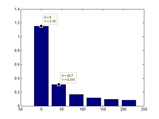
Однако это не означает, что стоит сразу бездумно увеличивать точность работы, т.к. это тоже приводит к негативным последствиям, т.к. если разрешение будет сопоставимо с частотой дискретизации сигнала, в спектр полезут гармоники «окна», которые имеют отношение не к реальному сигналу, а к его дискретному представлению:

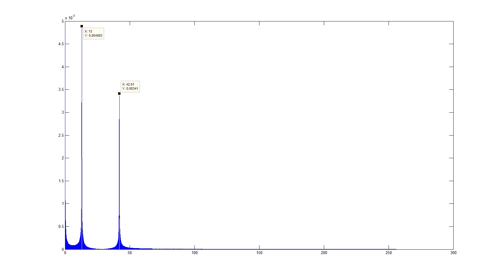
Или более близко окрестности одной из дискреток:

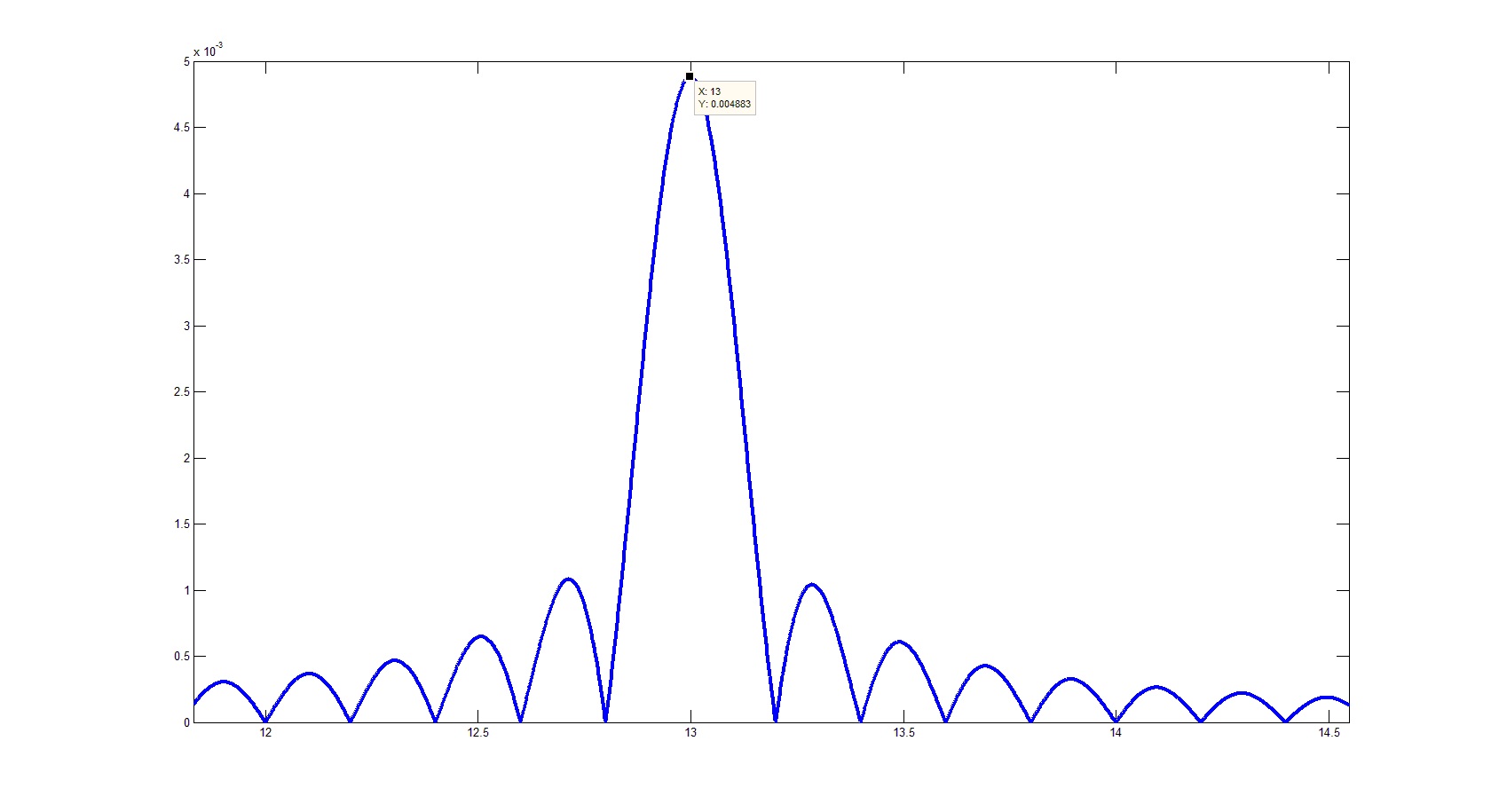
Код для нормировки fft будет выглядеть приблизительно следующим образом:

%% Спектральное представление сигнала FftS=abs(fft(Signal,FftL));% Амплитуды преобразования Фурье сигнала FftS=2*FftS./FftL;% Нормировка спектра по амплитуде FftS(1)=FftS(1)/2;% Нормировка постоянной составляющей в спектре FftSh=abs(fft(Signal+Noise,FftL));% Амплитуды преобразования Фурье смеси сигнал+шум FftSh=2*FftSh./FftL;% Нормировка спектра по амплитуде FftSh(1)=FftSh(1)/2;% Нормировка постоянной составляющей в спектре

Нам осталось только вывести результаты. Функция subplot позволяет разбить окно на несколько областей для отображения графиков.

%% Построение графиков subplot(2,1,1);% Выбор области окна для построения plot(T,Signal);% Построение сигнала title('Сигнал');% Подпись графика xlabel('Время (с)');% Подпись оси х графика ylabel('Амплитуда (Попугаи)');% Подпись оси у графика subplot(2,1,2);% Выбор области окна для построения plot(T,Signal+Noise);% Построение смеси сигнал+шум title('Сигнал+шум');% Подпись графика xlabel('Время (с)');% Подпись оси х графика ylabel('Амплитуда (Попугаи)');% Подпись оси у графика


F=0:Fd/FftL:Fd/2-1/FftL;% Массив частот вычисляемого спектра Фурье

figure% Создаем новое окно

subplot(2,1,1);% Выбор области окна для построения

plot(F,FftS(1:length(F)));% Построение спектра Фурье сигнала

title('Спектр сигнала');% Подпись графика

xlabel('Частота (Гц)');% Подпись оси х графика

ylabel('Амплитуда (Попугаи)');% Подпись оси у графика

subplot(2,1,2);% Выбор области окна для построения

plot(F,FftSh(1:length(F)));% Построение спектра Фурье сигнала

title('Спектр сигнала');% Подпись графика

xlabel('Частота (Гц)');% Подпись оси х графика

ylabel('Амплитуда (Попугаи)');% Подпись оси у графика

Результат выполнения кода будет выглядеть следующим образом:

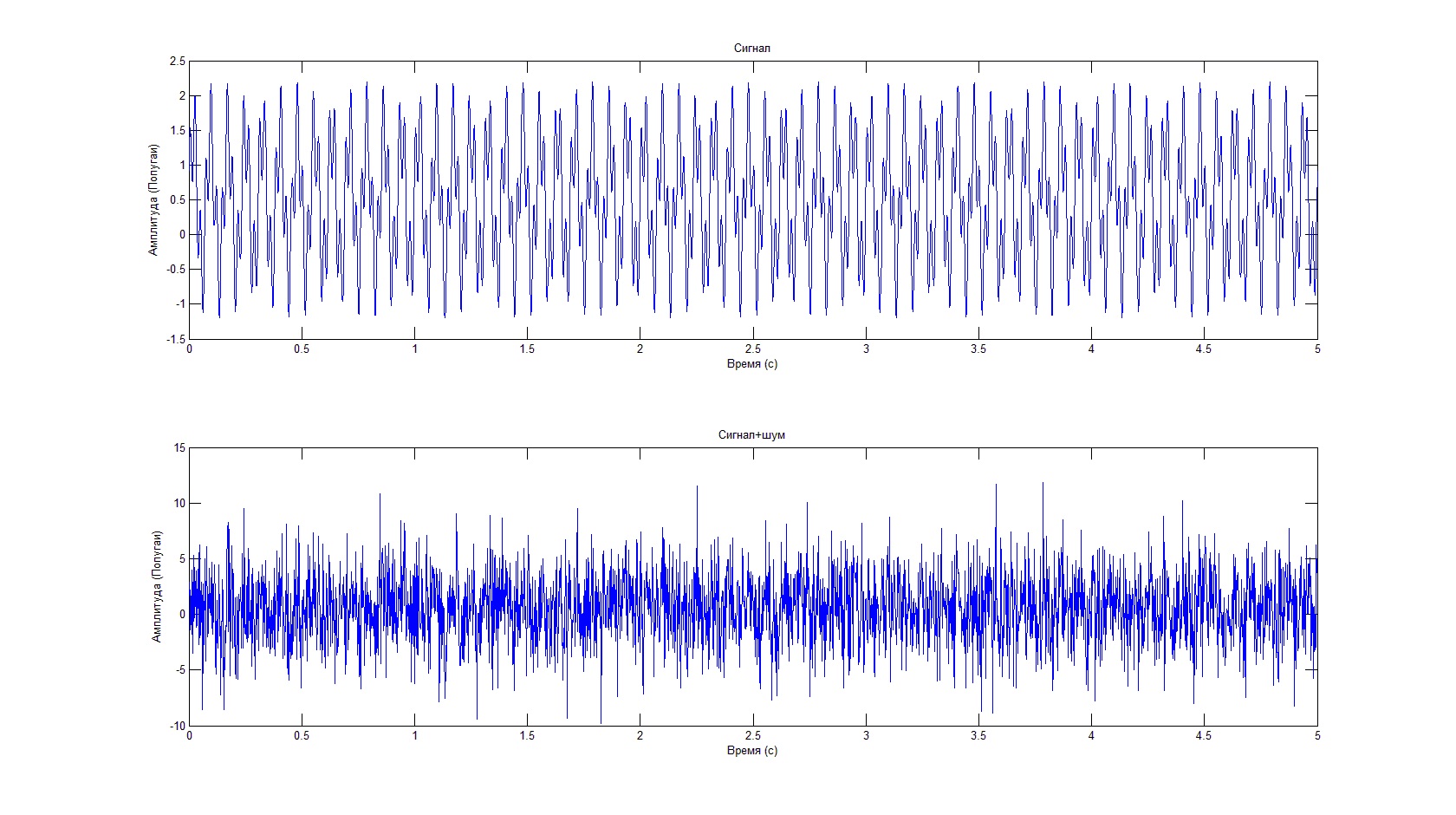
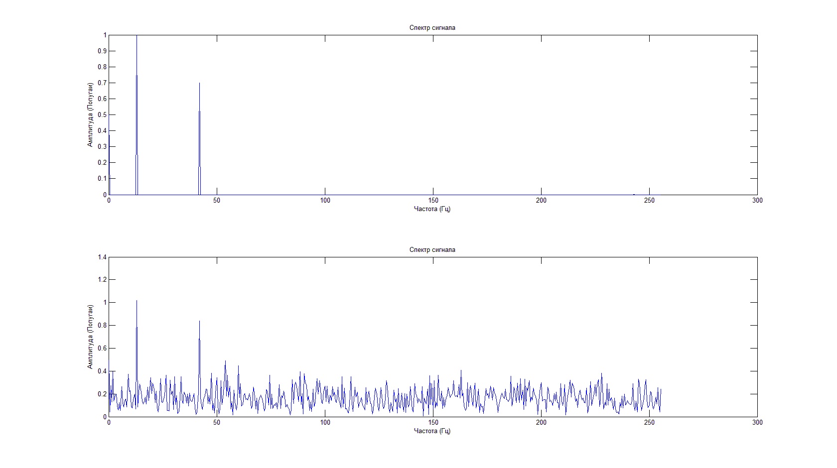
Несмотря на то, что полезного сигнала не видно на фоне шума, спектральная характеристика позволяет определить его частоту и амплитуду.

Надеюсь данный текст был вам полезен.

Источник

Основной спектральный анализ

Преобразование Фурье является инструментом для выполнения частоты и анализа спектра мощности сигналов временной области.

Количества спектрального анализа

Спектральный анализ изучает спектр частоты, содержавшийся в дискретном, однородно выборочных данных. Преобразование Фурье является инструментом, который показывает частотные составляющие времени — или основанный на пробеле сигнал путем представления его в пространстве частоты. В следующей таблице перечислены общие количества, используемые, чтобы охарактеризовать и интерпретировать свойства сигнала. Чтобы узнать больше о преобразовании Фурье, смотрите преобразования Фурье.

Количество	Описание
`x`	Выборочные данные
`n = length(x)`	Количество отсчетов
`fs`	Демонстрационная частота (выборки в единицу времени или пробел)
`dt = 1/fs`	Шаг времени или пространства на выборку
`t = (0:n-1)/fs`	Область значений времени или пространства для данных
`y = fft(x)`	Дискретное преобразование Фурье данных (ДПФ)
`abs(y)`	Амплитуда ДПФ
`(abs(y).^2)/n`	Степень ДПФ
`fs/n`	Шаг частоты
`f = (0:n-1)*(fs/n)`	Частотный диапазон
`fs/2`	Частота Найквиста (средняя точка частотного диапазона)

Сигнал с шумом

Преобразование Фурье может вычислить частотные составляющие сигнала, который повреждается случайным шумом.

Создайте сигнал с частотами компонента на уровне 15 Гц и 40 Гц, и введите случайный Гауссов шум.

rng('default')
fs = 100;                                % sample frequency (Hz)
t = 0:1/fs:10-1/fs;                      % 10 second span time vector
x = (1.3)*sin(2*pi*15*t) ...             % 15 Hz component
  + (1.7)*sin(2*pi*40*(t-2)) ...         % 40 Hz component
  + 2.5*randn(size(t));                  % Gaussian noise;

Преобразование Фурье сигнала идентифицирует свои частотные составляющие. В MATLAB®, fft функция вычисляет преобразование Фурье с помощью алгоритма быстрого преобразования Фурье. Используйте fft вычислить дискретное преобразование Фурье сигнала.

Постройте спектр мощности в зависимости от частоты. В то время как шум маскирует частотные составляющие сигнала на основанном на времени пробеле, преобразование Фурье показывает их как скачки в степени.

n = length(x);          % number of samples
f = (0:n-1)*(fs/n);     % frequency range
power = abs(y).^2/n;    % power of the DFT

plot(f,power)
xlabel('Frequency')
ylabel('Power')

Во многих приложениях более удобно просмотреть спектр мощности, сосредоточенный на 0 частотах, потому что это лучше представляет периодичность сигнала. Используйте fftshift функция, чтобы выполнить циклический сдвиг на y, и постройте степень в центре 0.

y0 = fftshift(y);         % shift y values
f0 = (-n/2:n/2-1)*(fs/n); % 0-centered frequency range
power0 = abs(y0).^2/n;    % 0-centered power

plot(f0,power0)
xlabel('Frequency')
ylabel('Power')

Звуковой сигнал

Можно использовать преобразование Фурье, чтобы анализировать спектр частоты аудиоданных.

Файл bluewhale.au содержит аудиоданные от Тихоокеанской вокализации голубого кита, зарегистрированной подводными микрофонами недалеко от берегов Калифорнии. Файл от библиотеки вокализаций животных, обеспеченных Программой исследований Биоакустики Корнелльского университета.

Поскольку вызовы голубого кита являются настолько низкими, они являются едва слышимыми людям. Масштаб времени в данных сжат на коэффициент 10, чтобы повысить тангаж и выполнить более явно слышимый вызов. Считайте и постройте аудиоданные. Можно использовать команду sound(x,fs) слушать аудио.

whaleFile = 'bluewhale.au';
[x,fs] = audioread(whaleFile);

plot(x)
xlabel('Sample Number')
ylabel('Amplitude')

Первый звук является «трелью», сопровождаемой тремя «стонами». Этот пример анализирует один стон. Задайте новые данные, которые приблизительно состоят из первого стона, и откорректируйте данные времени с учетом factor-10 ускорения. Постройте усеченный сигнал в зависимости от времени.

moan = x(2.45e4:3.10e4);
t = 10*(0:1/fs:(length(moan)-1)/fs);

plot(t,moan)
xlabel('Time (seconds)')
ylabel('Amplitude')
xlim([0 t(end)])

Преобразование Фурье данных идентифицирует частотные составляющие звукового сигнала. В некоторых приложениях, что процесс большие объемы данных с fft, распространено изменить размер входа так, чтобы количество отсчетов было степенью 2. Это может сделать расчет преобразования значительно быстрее, особенно для объемов выборки с большими простыми множителями. Задайте новую длину сигнала n это — степень 2, и используйте fft функция, чтобы вычислить дискретное преобразование Фурье сигнала. fft автоматически заполняет исходные данные нулями, чтобы увеличить объем выборки.

m = length(moan);       % original sample length
n = pow2(nextpow2(m));  % transform length
y = fft(moan,n);        % DFT of signal

Настройте частотный диапазон из-за фактора ускорения, и вычислите и постройте спектр мощности сигнала. График показывает, что стон состоит из основной частоты приблизительно 17 Гц и последовательности гармоник, где вторая гармоника подчеркнута.

f = (0:n-1)*(fs/n)/10;
power = abs(y).^2/n;      

plot(f(1:floor(n/2)),power(1:floor(n/2)))
xlabel('Frequency')
ylabel('Power')

Смотрите также

Spectral Analysis Quantities

Noisy Signal

Audio Signal

See Also

Related Topics

Syntax

Description

Examples

Default Values of Spectrogram

Compare spectrogram Function and STFT Definition

Compare spectrogram and stft Functions

Spectrogram and Instantaneous Frequency

Spectrogram of Complex Signal

Compare spectrogram and pspectrum Functions

Reassigned Spectrogram of Quadratic Chirp

Spectrogram with Threshold

Compute Centered and One-Sided Spectrograms

Compute Segment PSDs and Power Spectra

Track Chirps in Audio Signal

3D Spectrogram Visualization

Input Arguments

x — Input signal vector

window — Window integer | vector | []

noverlap — Number of overlapped samples positive integer | []

nfft — Number of DFT points positive integer scalar | []

w — Normalized frequencies vector

f — Cyclical frequencies vector

fs — Sample rate 1 Hz (default) | positive scalar

freqrange — Frequency range for PSD estimate "onesided" | "twosided" | "centered"

spectrumtype — Power spectrum scaling "psd" (default) | "power"

freqloc — Frequency display axis "xaxis" (default) | "yaxis"

Name-Value Arguments

MinThreshold — Threshold -Inf (default) | real scalar

OutputTimeDimension — Output time dimension "acrosscolumns" (default) | "downrows"

Output Arguments

s — Short-time Fourier transform matrix

w — Normalized frequencies vector

t — Time instants vector

f — Cyclical frequencies vector

ps — Power spectral density or power spectrum matrix

fc, tc — Center-of-energy frequencies and times matrices

More About

Short-Time Fourier Transform

Tips

References

Extended Capabilities

Tall Arrays Calculate with arrays that have more rows than fit in memory.

C/C++ Code Generation Generate C and C++ code using MATLAB® Coder™.

Thread-Based Environment Run code in the background using MATLAB® backgroundPool or accelerate code with Parallel Computing Toolbox™ ThreadPool.

GPU Arrays Accelerate code by running on a graphics processing unit (GPU) using Parallel Computing Toolbox™.

Version History

R2023a: Visualize function outputs using Create Plot Live Editor task

See Also

Apps

Functions

Topics

pspectrum

Syntax

Description

Examples

Power Spectra of Sinusoids

Two-Sided Spectra

Window Leakage and Tone Resolution

Compare spectrogram and pspectrum Functions

Persistence Spectrum of Transient Signal

Spectrogram and Reassigned Spectrogram of Chirp

Spectrogram of Dial Tone Signal

Input Arguments

x — Input signal vector | matrix | timetable

fs — Sample rate 2π (default) | positive numeric scalar

t — Time values vector | datetime array | duration array | duration scalar

type — Type of spectrum to compute 'power' (default) | 'spectrogram' | 'persistence'

Name-Value Arguments

FrequencyLimits — Frequency band limits [0 fs/2] (default) | two-element numeric vector

FrequencyResolution — Frequency resolution bandwidth real numeric scalar

Leakage — Spectral leakage 0.5 (default) | real numeric scalar between 0 and 1

MinThreshold — Lower bound for nonzero values -Inf (default) | real scalar

NumPowerBins — Number of power bins for persistence spectrum 256 (default) | integer between 20 and 1024

OverlapPercent — Overlap between adjoining segments real scalar in the interval [0, 100)

Reassign — Reassignment option false (default) | true

Compare `spectrogram` Function and STFT Definition

Compare `spectrogram` and `stft` Functions

Compare `spectrogram` and `pspectrum` Functions

`x` — Input signal
vector

`window` — Window
integer | vector | `[]`

`noverlap` — Number of overlapped samples
positive integer | `[]`

`nfft` — Number of DFT points
positive integer scalar | `[]`

`w` — Normalized frequencies
vector

`f` — Cyclical frequencies
vector

`fs` — Sample rate
1 Hz (default) | positive scalar

`freqrange` — Frequency range for PSD estimate
`"onesided"`
| `"twosided"` | `"centered"`

`spectrumtype` — Power spectrum scaling
`"psd"` (default) | `"power"`

`freqloc` — Frequency display axis
`"xaxis"` (default) | `"yaxis"`

`MinThreshold` — Threshold
`-Inf` (default) | real scalar

`OutputTimeDimension` — Output time dimension
`"acrosscolumns"` (default) | `"downrows"`

`s` — Short-time Fourier transform
matrix

`w` — Normalized frequencies
vector

`t` — Time instants
vector

`f` — Cyclical frequencies
vector

`ps` — Power spectral density or power spectrum
matrix

`fc`, `tc` — Center-of-energy frequencies and times
matrices

Tall Arrays
Calculate with arrays that have more rows than fit in memory.

C/C++ Code Generation
Generate C and C++ code using MATLAB® Coder™.

Thread-Based Environment
Run code in the background using MATLAB® `backgroundPool` or accelerate code with Parallel Computing Toolbox™ `ThreadPool`.

GPU Arrays
Accelerate code by running on a graphics processing unit (GPU) using Parallel Computing Toolbox™.

R2023a: Visualize function outputs using Create Plot
Live Editor task

Compare `spectrogram` and `pspectrum` Functions

`x` — Input signal
vector | matrix | timetable

`fs` — Sample rate
2π (default) | positive numeric scalar

`t` — Time values
vector | `datetime` array | `duration` array | `duration` scalar

`type` — Type of spectrum to compute
`'power'` (default) | `'spectrogram'` | `'persistence'`

`FrequencyLimits` — Frequency band limits
`[0 fs/2]` (default) | two-element numeric vector

`FrequencyResolution` — Frequency resolution bandwidth
real numeric scalar

`Leakage` — Spectral leakage
`0.5` (default) | real numeric scalar between 0 and 1

`MinThreshold` — Lower bound for nonzero values
`-Inf` (default) | real scalar

`NumPowerBins` — Number of power bins for persistence spectrum
`256` (default) | integer between 20 and 1024

`OverlapPercent` — Overlap between adjoining segments
real scalar in the interval [0, 100)

`Reassign` — Reassignment option
`false` (default) | `true`

`TimeResolution` — Time resolution of spectrogram or persistence spectrum
real scalar

`TwoSided` — Two-sided spectral estimate
false | true

`p` — Spectrum
vector | matrix

`f` — Spectrum frequencies
vector

`t` — Time values of spectrogram
vector | `datetime` array | `duration` array

`pwr` — Power values of persistence spectrum
vector

C/C++ Code Generation
Generate C and C++ code using MATLAB® Coder™.

GPU Arrays
Accelerate code by running on a graphics processing unit (GPU) using Parallel Computing Toolbox™.