Как найти среднюю гармоническую скорость - Исправление недочетов и поиск решений вместе с Examum.ru

In mathematics, the harmonic mean is one of several kinds of average, and in particular, one of the Pythagorean means. It is sometimes appropriate for situations when the average rate is desired.^[1]

The harmonic mean can be expressed as the reciprocal of the arithmetic mean of the reciprocals of the given set of observations. As a simple example, the harmonic mean of 1, 4, and 4 is

${displaystyle left({frac {1^{-1}+4^{-1}+4^{-1}}{3}}right)^{-1}={frac {3}{{frac {1}{1}}+{frac {1}{4}}+{frac {1}{4}}}}={frac {3}{1.5}}=2,.}$

Definition[edit]

The harmonic mean H of the positive real numbers
$x_{1},x_{2},ldots ,x_{n}$ is defined to be

${displaystyle H={frac {n}{{frac {1}{x_{1}}}+{frac {1}{x_{2}}}+cdots +{frac {1}{x_{n}}}}}={frac {n}{sum limits _{i=1}^{n}{frac {1}{x_{i}}}}}=left({frac {sum limits _{i=1}^{n}x_{i}^{-1}}{n}}right)^{-1}.}$

The third formula in the above equation expresses the harmonic mean as the reciprocal of the arithmetic mean of the reciprocals.

From the following formula:

${displaystyle H={frac {ncdot prod limits _{j=1}^{n}x_{j}}{sum limits _{i=1}^{n}left{{frac {1}{x_{i}}}{prod limits _{j=1}^{n}x_{j}}right}}}.}$

it is more apparent that the harmonic mean is related to the arithmetic and geometric means. It is the reciprocal dual of the arithmetic mean for positive inputs:

${displaystyle 1/H(1/x_{1}ldots 1/x_{n})=A(x_{1}ldots x_{n})}$

The harmonic mean is a Schur-concave function, and dominated by the minimum of its arguments, in the sense that for any positive set of arguments, ${displaystyle min(x_{1}ldots x_{n})leq H(x_{1}ldots x_{n})leq nmin(x_{1}ldots x_{n})}$ . Thus, the harmonic mean cannot be made arbitrarily large by changing some values to bigger ones (while having at least one value unchanged).

The harmonic mean is also concave, which is an even stronger property than Schur-concavity.
One has to take care to only use positive numbers though, since the mean fails to be concave if negative values are used.

Relationship with other means[edit]

The harmonic mean is one of the three Pythagorean means. For all positive data sets containing at least one pair of nonequal values, the harmonic mean is always the least of the three means,^[2] while the arithmetic mean is always the greatest of the three and the geometric mean is always in between. (If all values in a nonempty dataset are equal, the three means are always equal to one another; e.g., the harmonic, geometric, and arithmetic means of {2, 2, 2} are all 2.)

It is the special case M₋₁ of the power mean:

${displaystyle Hleft(x_{1},x_{2},ldots ,x_{n}right)=M_{-1}left(x_{1},x_{2},ldots ,x_{n}right)={frac {n}{x_{1}^{-1}+x_{2}^{-1}+cdots +x_{n}^{-1}}}}$

Since the harmonic mean of a list of numbers tends strongly toward the least elements of the list, it tends (compared to the arithmetic mean) to mitigate the impact of large outliers and aggravate the impact of small ones.

The arithmetic mean is often mistakenly used in places calling for the harmonic mean.^[3] In the speed example below for instance, the arithmetic mean of 40 is incorrect, and too big.

The harmonic mean is related to the other Pythagorean means, as seen in the equation below. This can be seen by interpreting the denominator to be the arithmetic mean of the product of numbers n times but each time omitting the j-th term. That is, for the first term, we multiply all n numbers except the first; for the second, we multiply all n numbers except the second; and so on. The numerator, excluding the n, which goes with the arithmetic mean, is the geometric mean to the power n. Thus the n-th harmonic mean is related to the n-th geometric and arithmetic means. The general formula is

${displaystyle Hleft(x_{1},ldots ,x_{n}right)={frac {left(Gleft(x_{1},ldots ,x_{n}right)right)^{n}}{Aleft(x_{2}x_{3}cdots x_{n},x_{1}x_{3}cdots x_{n},ldots ,x_{1}x_{2}cdots x_{n-1}right)}}={frac {left(Gleft(x_{1},ldots ,x_{n}right)right)^{n}}{Aleft({frac {1}{x_{1}}}{prod limits _{i=1}^{n}x_{i}},{frac {1}{x_{2}}}{prod limits _{i=1}^{n}x_{i}},ldots ,{frac {1}{x_{n}}}{prod limits _{i=1}^{n}x_{i}}right)}}.}$

If a set of non-identical numbers is subjected to a mean-preserving spread — that is, two or more elements of the set are «spread apart» from each other while leaving the arithmetic mean unchanged — then the harmonic mean always decreases.^[4]

Harmonic mean of two or three numbers[edit]

Two numbers[edit]

For the special case of just two numbers, $x_{1}$ and $x_{2}$ , the harmonic mean can be written

${displaystyle H={frac {2x_{1}x_{2}}{x_{1}+x_{2}}}qquad }$

or ${displaystyle qquad {frac {1}{H}}={frac {(1/x_{1})+(1/x_{2})}{2}}.}$

In this special case, the harmonic mean is related to the arithmetic mean $A={frac {x_{1}+x_{2}}{2}}$ and the geometric mean $G={sqrt {x_{1}x_{2}}},$ by

${displaystyle H={frac {G^{2}}{A}}=Gleft({frac {G}{A}}right).}$

Since ${displaystyle {tfrac {G}{A}}leq 1}$ by the inequality of arithmetic and geometric means, this shows for the n = 2 case that H ≤ G (a property that in fact holds for all n). It also follows that , meaning the two numbers’ geometric mean equals the geometric mean of their arithmetic and harmonic means.

Three numbers[edit]

For the special case of three numbers, $x_{1}$ , $x_{2}$ and $x_{3}$ , the harmonic mean can be written

${displaystyle H={frac {3x_{1}x_{2}x_{3}}{x_{1}x_{2}+x_{1}x_{3}+x_{2}x_{3}}}.}$

Three positive numbers H, G, and A are respectively the harmonic, geometric, and arithmetic means of three positive numbers if and only if^[5]^{: p.74, #1834} the following inequality holds

${displaystyle {frac {A^{3}}{G^{3}}}+{frac {G^{3}}{H^{3}}}+1leq {frac {3}{4}}left(1+{frac {A}{H}}right)^{2}.}$

Weighted harmonic mean[edit]

If a set of weights $w_{1}$ , …, $w_{n}$ is associated to the dataset $x_{1}$ , …, $x_{n}$ , the weighted harmonic mean is defined by ^[6]

${displaystyle H={frac {sum limits _{i=1}^{n}w_{i}}{sum limits _{i=1}^{n}{frac {w_{i}}{x_{i}}}}}=left({frac {sum limits _{i=1}^{n}w_{i}x_{i}^{-1}}{sum limits _{i=1}^{n}w_{i}}}right)^{-1}.}$

The unweighted harmonic mean can be regarded as the special case where all of the weights are equal.

Examples[edit]

In physics[edit]

Average speed[edit]

In many situations involving rates and ratios, the harmonic mean provides the correct average. For instance, if a vehicle travels a certain distance d outbound at a speed x (e.g. 60 km/h) and returns the same distance at a speed y (e.g. 20 km/h), then its average speed is the harmonic mean of x and y (30 km/h), not the arithmetic mean (40 km/h). The total travel time is the same as if it had traveled the whole distance at that average speed. This can be proven as follows:^[7]

Average speed for the entire journey
= Total distance traveled/Sum of time for each segment
= 2d/d/x + d/y = 2/1/x+1/y

However, if the vehicle travels for a certain amount of time at a speed x and then the same amount of time at a speed y, then its average speed is the arithmetic mean of x and y, which in the above example is 40 km/h.

Average speed for the entire journey
= Total distance traveled/Sum of time for each segment
= xt+yt/2t
= x+y/2

The same principle applies to more than two segments: given a series of sub-trips at different speeds, if each sub-trip covers the same distance, then the average speed is the harmonic mean of all the sub-trip speeds; and if each sub-trip takes the same amount of time, then the average speed is the arithmetic mean of all the sub-trip speeds. (If neither is the case, then a weighted harmonic mean or weighted arithmetic mean is needed. For the arithmetic mean, the speed of each portion of the trip is weighted by the duration of that portion, while for the harmonic mean, the corresponding weight is the distance. In both cases, the resulting formula reduces to dividing the total distance by the total time.)

However, one may avoid the use of the harmonic mean for the case of «weighting by distance». Pose the problem as finding «slowness» of the trip where «slowness» (in hours per kilometre) is the inverse of speed. When trip slowness is found, invert it so as to find the «true» average trip speed. For each trip segment i, the slowness s_i = 1/speed_i. Then take the weighted arithmetic mean of the s_i‘s weighted by their respective distances (optionally with the weights normalized so they sum to 1 by dividing them by trip length). This gives the true average slowness (in time per kilometre). It turns out that this procedure, which can be done with no knowledge of the harmonic mean, amounts to the same mathematical operations as one would use in solving this problem by using the harmonic mean. Thus it illustrates why the harmonic mean works in this case.

Density[edit]

Similarly, if one wishes to estimate the density of an alloy given the densities of its constituent elements and their mass fractions (or, equivalently, percentages by mass), then the predicted density of the alloy (exclusive of typically minor volume changes due to atom packing effects) is the weighted harmonic mean of the individual densities, weighted by mass, rather than the weighted arithmetic mean as one might at first expect. To use the weighted arithmetic mean, the densities would have to be weighted by volume. Applying dimensional analysis to the problem while labeling the mass units by element and making sure that only like element-masses cancel makes this clear.

Electricity[edit]

If one connects two electrical resistors in parallel, one having resistance x (e.g., 60 Ω) and one having resistance y (e.g., 40 Ω), then the effect is the same as if one had used two resistors with the same resistance, both equal to the harmonic mean of x and y (48 Ω): the equivalent resistance, in either case, is 24 Ω (one-half of the harmonic mean). This same principle applies to capacitors in series or to inductors in parallel.

However, if one connects the resistors in series, then the average resistance is the arithmetic mean of x and y (50 Ω), with total resistance equal to twice this, the sum of x and y (100 Ω). This principle applies to capacitors in parallel or to inductors in series.

As with the previous example, the same principle applies when more than two resistors, capacitors or inductors are connected, provided that all are in parallel or all are in series.

The «conductivity effective mass» of a semiconductor is also defined as the harmonic mean of the effective masses along the three crystallographic directions.^[8]

Optics[edit]

As for other optic equations, the thin lens equation 1/f = 1/u + 1/v can be rewritten such that the focal length f is one-half of the harmonic mean of the distances of the subject u and object v from the lens.^[9]

In finance[edit]

The weighted harmonic mean is the preferable method for averaging multiples, such as the price–earnings ratio (P/E). If these ratios are averaged using a weighted arithmetic mean, high data points are given greater weights than low data points. The weighted harmonic mean, on the other hand, correctly weights each data point.^[10] The simple weighted arithmetic mean when applied to non-price normalized ratios such as the P/E is biased upwards and cannot be numerically justified, since it is based on equalized earnings; just as vehicles speeds cannot be averaged for a roundtrip journey (see above).^[11]

For example, consider two firms, one with a market capitalization of $150 billion and earnings of $5 billion (P/E of 30) and one with a market capitalization of $1 billion and earnings of $1 million (P/E of 1000). Consider an index made of the two stocks, with 30% invested in the first and 70% invested in the second. We want to calculate the P/E ratio of this index.

Using the weighted arithmetic mean (incorrect):

{displaystyle P/E=0.3times 30+0.7times 1000=709}

Using the weighted harmonic mean (correct):

${displaystyle P/E={frac {0.3+0.7}{0.3/30+0.7/1000}}approx 93.46}$

Thus, the correct P/E of 93.46 of this index can only be found using the weighted harmonic mean, while the weighted arithmetic mean will significantly overestimate it.

In geometry[edit]

In any triangle, the radius of the incircle is one-third of the harmonic mean of the altitudes.

For any point P on the minor arc BC of the circumcircle of an equilateral triangle ABC, with distances q and t from B and C respectively, and with the intersection of PA and BC being at a distance y from point P, we have that y is half the harmonic mean of q and t.^[12]

In a right triangle with legs a and b and altitude h from the hypotenuse to the right angle, h² is half the harmonic mean of a² and b².^[13]^[14]

Let t and s (t > s) be the sides of the two inscribed squares in a right triangle with hypotenuse c. Then s² equals half the harmonic mean of c² and t².

Let a trapezoid have vertices A, B, C, and D in sequence and have parallel sides AB and CD. Let E be the intersection of the diagonals, and let F be on side DA and G be on side BC such that FEG is parallel to AB and CD. Then FG is the harmonic mean of AB and DC. (This is provable using similar triangles.)

Crossed ladders. h is half the harmonic mean of A and B

One application of this trapezoid result is in the crossed ladders problem, where two ladders lie oppositely across an alley, each with feet at the base of one sidewall, with one leaning against a wall at height A and the other leaning against the opposite wall at height B, as shown. The ladders cross at a height of h above the alley floor. Then h is half the harmonic mean of A and B. This result still holds if the walls are slanted but still parallel and the «heights» A, B, and h are measured as distances from the floor along lines parallel to the walls. This can be proved easily using the area formula of a trapezoid and area addition formula.

In an ellipse, the semi-latus rectum (the distance from a focus to the ellipse along a line parallel to the minor axis) is the harmonic mean of the maximum and minimum distances of the ellipse from a focus.

In other sciences[edit]

In computer science, specifically information retrieval and machine learning, the harmonic mean of the precision (true positives per predicted positive) and the recall (true positives per real positive) is often used as an aggregated performance score for the evaluation of algorithms and systems: the F-score (or F-measure). This is used in information retrieval because only the positive class is of relevance, while number of negatives, in general, is large and unknown.^[15] It is thus a trade-off as to whether the correct positive predictions should be measured in relation to the number of predicted positives or the number of real positives, so it is measured versus a putative number of positives that is an arithmetic mean of the two possible denominators.

A consequence arises from basic algebra in problems where people or systems work together. As an example, if a gas-powered pump can drain a pool in 4 hours and a battery-powered pump can drain the same pool in 6 hours, then it will take both pumps 6·4/6 + 4, which is equal to 2.4 hours, to drain the pool together. This is one-half of the harmonic mean of 6 and 4: 2·6·4/6 + 4 = 4.8. That is, the appropriate average for the two types of pump is the harmonic mean, and with one pair of pumps (two pumps), it takes half this harmonic mean time, while with two pairs of pumps (four pumps) it would take a quarter of this harmonic mean time.

In hydrology, the harmonic mean is similarly used to average hydraulic conductivity values for a flow that is perpendicular to layers (e.g., geologic or soil) — flow parallel to layers uses the arithmetic mean. This apparent difference in averaging is explained by the fact that hydrology uses conductivity, which is the inverse of resistivity.

In sabermetrics, a baseball player’s Power–speed number is the harmonic mean of their home run and stolen base totals.

In population genetics, the harmonic mean is used when calculating the effects of fluctuations in the census population size on the effective population size. The harmonic mean takes into account the fact that events such as population bottleneck increase the rate genetic drift and reduce the amount of genetic variation in the population. This is a result of the fact that following a bottleneck very few individuals contribute to the gene pool limiting the genetic variation present in the population for many generations to come.

When considering fuel economy in automobiles two measures are commonly used – miles per gallon (mpg), and litres per 100 km. As the dimensions of these quantities are the inverse of each other (one is distance per volume, the other volume per distance) when taking the mean value of the fuel economy of a range of cars one measure will produce the harmonic mean of the other – i.e., converting the mean value of fuel economy expressed in litres per 100 km to miles per gallon will produce the harmonic mean of the fuel economy expressed in miles per gallon. For calculating the average fuel consumption of a fleet of vehicles from the individual fuel consumptions, the harmonic mean should be used if the fleet uses miles per gallon, whereas the arithmetic mean should be used if the fleet uses litres per 100 km. In the USA the CAFE standards (the federal automobile fuel consumption standards) make use of the harmonic mean.

In chemistry and nuclear physics the average mass per particle of a mixture consisting of different species (e.g., molecules or isotopes) is given by the harmonic mean of the individual species’ masses weighted by their respective mass fraction.

Beta distribution[edit]

Harmonic mean for Beta distribution for 0 < α < 5 and 0 < β < 5

(Mean — HarmonicMean) for Beta distribution versus alpha and beta from 0 to 2

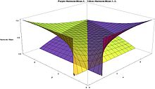
Harmonic Means for Beta distribution Purple=H(X), Yellow=H(1-X), smaller values alpha and beta in front

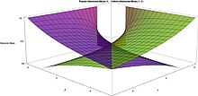
Harmonic Means for Beta distribution Purple=H(X), Yellow=H(1-X), larger values alpha and beta in front

The harmonic mean of a beta distribution with shape parameters α and β is:

${displaystyle H={frac {alpha -1}{alpha +beta -1}}{text{ conditional on }}alpha >1,,&,,beta >0}$

The harmonic mean with α < 1 is undefined because its defining expression is not bounded in [0, 1].

Letting α = β

${displaystyle H={frac {alpha -1}{2alpha -1}}}$

showing that for α = β the harmonic mean ranges from 0 for α = β = 1, to 1/2 for α = β → ∞.

The following are the limits with one parameter finite (non-zero) and the other parameter approaching these limits:

${displaystyle {begin{aligned}lim _{alpha to 0}H&={text{ undefined }}\lim _{alpha to 1}H&=lim _{beta to infty }H=0\lim _{beta to 0}H&=lim _{alpha to infty }H=1end{aligned}}}$

With the geometric mean the harmonic mean may be useful in maximum likelihood estimation in the four parameter case.

A second harmonic mean (H_{1 − X}) also exists for this distribution

${displaystyle H_{1-X}={frac {beta -1}{alpha +beta -1}}{text{ conditional on }}beta >1,,&,,alpha >0}$

This harmonic mean with β < 1 is undefined because its defining expression is not bounded in [ 0, 1 ].

Letting α = β in the above expression

${displaystyle H_{1-X}={frac {beta -1}{2beta -1}}}$

showing that for α = β the harmonic mean ranges from 0, for α = β = 1, to 1/2, for α = β → ∞.

The following are the limits with one parameter finite (non zero) and the other approaching these limits:

${displaystyle {begin{aligned}lim _{beta to 0}H_{1-X}&={text{ undefined }}\lim _{beta to 1}H_{1-X}&=lim _{alpha to infty }H_{1-X}=0\lim _{alpha to 0}H_{1-X}&=lim _{beta to infty }H_{1-X}=1end{aligned}}}$

Although both harmonic means are asymmetric, when α = β the two means are equal.

Lognormal distribution[edit]

The harmonic mean ( H ) of the lognormal distribution of a random variable X is^[16]

${displaystyle H=exp left(mu -{frac {1}{2}}sigma ^{2}right),}$

where μ and σ² are the parameters of the distribution, i.e. the mean and variance of the distribution of the natural logarithm of X.

The harmonic and arithmetic means of the distribution are related by

${displaystyle {frac {mu ^{*}}{H}}=1+C_{v}^{2},,}$

where C_v and μ^* are the coefficient of variation and the mean of the distribution respectively..

The geometric (G), arithmetic and harmonic means of the distribution are related by^[17]

${displaystyle Hmu ^{*}=G^{2}.}$

Pareto distribution[edit]

The harmonic mean of type 1 Pareto distribution is^[18]

${displaystyle H=kleft(1+{frac {1}{alpha }}right)}$

where k is the scale parameter and α is the shape parameter.

Statistics[edit]

For a random sample, the harmonic mean is calculated as above. Both the mean and the variance may be infinite (if it includes at least one term of the form 1/0).

Sample distributions of mean and variance[edit]

The mean of the sample m is asymptotically distributed normally with variance s².

${displaystyle s^{2}={frac {mleft[operatorname {E} left({frac {1}{x}}-1right)right]}{m^{2}n}}}$

The variance of the mean itself is^[19]

${displaystyle operatorname {Var} left({frac {1}{x}}right)={frac {mleft[operatorname {E} left({frac {1}{x}}-1right)right]}{nm^{2}}}}$

where m is the arithmetic mean of the reciprocals, x are the variates, n is the population size and E is the expectation operator.

Delta method[edit]

Assuming that the variance is not infinite and that the central limit theorem applies to the sample then using the delta method, the variance is

${displaystyle operatorname {Var} (H)={frac {1}{n}}{frac {s^{2}}{m^{4}}}}$

where H is the harmonic mean, m is the arithmetic mean of the reciprocals

${displaystyle m={frac {1}{n}}sum {frac {1}{x}}.}$

s² is the variance of the reciprocals of the data

${displaystyle s^{2}=operatorname {Var} left({frac {1}{x}}right)}$

and n is the number of data points in the sample.

Jackknife method[edit]

A jackknife method of estimating the variance is possible if the mean is known.^[20] This method is the usual ‘delete 1’ rather than the ‘delete m’ version.

This method first requires the computation of the mean of the sample (m)

${displaystyle m={frac {n}{sum {frac {1}{x}}}}}$

where x are the sample values.

A series of value w_i is then computed where

${displaystyle w_{i}={frac {n-1}{sum _{jneq i}{frac {1}{x}}}}.}$

The mean (h) of the w_i is then taken:

${displaystyle h={frac {1}{n}}sum {w_{i}}}$

The variance of the mean is

${displaystyle {frac {n-1}{n}}sum {(m-w_{i})}^{2}.}$

Significance testing and confidence intervals for the mean can then be estimated with the t test.

Size biased sampling[edit]

Assume a random variate has a distribution f( x ). Assume also that the likelihood of a variate being chosen is proportional to its value. This is known as length based or size biased sampling.

Let μ be the mean of the population. Then the probability density function f*( x ) of the size biased population is

${displaystyle f^{*}(x)={frac {xf(x)}{mu }}}$

The expectation of this length biased distribution E^*( x ) is^[19]

${displaystyle operatorname {E} ^{*}(x)=mu left[1+{frac {sigma ^{2}}{mu ^{2}}}right]}$

where σ² is the variance.

The expectation of the harmonic mean is the same as the non-length biased version E( x )

${displaystyle E^{*}(x^{-1})=E(x)^{-1}}$

The problem of length biased sampling arises in a number of areas including textile manufacture^[21] pedigree analysis^[22] and survival analysis^[23]

Akman et al. have developed a test for the detection of length based bias in samples.^[24]

Shifted variables[edit]

If X is a positive random variable and q > 0 then for all ε > 0^[25]

${displaystyle operatorname {Var} left[{frac {1}{(X+epsilon )^{q}}}right]<operatorname {Var} left({frac {1}{X^{q}}}right).}$

Moments[edit]

Assuming that X and E(X) are > 0 then^[25]

${displaystyle operatorname {E} left[{frac {1}{X}}right]geq {frac {1}{operatorname {E} (X)}}}$

This follows from Jensen’s inequality.

Gurland has shown that^[26] for a distribution that takes only positive values, for any n > 0

${displaystyle operatorname {E} left(X^{-1}right)geq {frac {operatorname {E} left(X^{n-1}right)}{operatorname {E} left(X^{n}right)}}.}$

Under some conditions^[27]

${displaystyle operatorname {E} (a+X)^{-n}sim operatorname {E} left(a+X^{-n}right)}$

where ~ means approximately equal to.

Sampling properties[edit]

Assuming that the variates (x) are drawn from a lognormal distribution there are several possible estimators for H:

${displaystyle {begin{aligned}H_{1}&={frac {n}{sum left({frac {1}{x}}right)}}\H_{2}&={frac {left(exp left[{frac {1}{n}}sum log _{e}(x)right]right)^{2}}{{frac {1}{n}}sum (x)}}\H_{3}&=exp left(m-{frac {1}{2}}s^{2}right)end{aligned}}}$

where

${displaystyle m={frac {1}{n}}sum log _{e}(x)}$

${displaystyle s^{2}={frac {1}{n}}sum left(log _{e}(x)-mright)^{2}}$

Of these H₃ is probably the best estimator for samples of 25 or more.^[28]

Bias and variance estimators[edit]

A first order approximation to the bias and variance of H₁ are^[29]

${displaystyle {begin{aligned}operatorname {bias} left[H_{1}right]&={frac {HC_{v}}{n}}\operatorname {Var} left[H_{1}right]&={frac {H^{2}C_{v}}{n}}end{aligned}}}$

where C_v is the coefficient of variation.

Similarly a first order approximation to the bias and variance of H₃ are^[29]

${displaystyle {begin{aligned}{frac {Hlog _{e}left(1+C_{v}right)}{2n}}left[1+{frac {1+C_{v}^{2}}{2}}right]\{frac {Hlog _{e}left(1+C_{v}right)}{n}}left[1+{frac {1+C_{v}^{2}}{4}}right]end{aligned}}}$

In numerical experiments H₃ is generally a superior estimator of the harmonic mean than H₁.^[29] H₂ produces estimates that are largely similar to H₁.

Notes[edit]

The Environmental Protection Agency recommends the use of the harmonic mean in setting maximum toxin levels in water.^[30]

In geophysical reservoir engineering studies, the harmonic mean is widely used.^[31]

Notes[edit]

^ If AC = a and BC = b. OC = AM of a and b, and radius r = QO = OG.
Using Pythagoras’ theorem, QC² = QO² + OC² ∴ QC = √QO² + OC² = QM.
Using Pythagoras’ theorem, OC² = OG² + GC² ∴ GC = √OC² − OG² = GM.
Using similar triangles, HC/GC = GC/OC ∴ HC = GC²/OC = HM.

References[edit]

^ https://www.comap.com/FloydVest/Course/PDF/Cons25PO.pdf Archived 2022-07-11 at the Wayback Machine^{[bare URL PDF]}
^ Da-Feng Xia, Sen-Lin Xu, and Feng Qi, «A proof of the arithmetic mean-geometric mean-harmonic mean inequalities», RGMIA Research Report Collection, vol. 2, no. 1, 1999, http://ajmaa.org/RGMIA/papers/v2n1/v2n1-10.pdf Archived 2015-12-22 at the Wayback Machine
^ *Statistical Analysis, Ya-lun Chou, Holt International, 1969, ISBN 0030730953
^ Mitchell, Douglas W., «More on spreads and non-arithmetic means,» The Mathematical Gazette 88, March 2004, 142–144.
^ Inequalities proposed in “Crux Mathematicorum”, «Archived copy» (PDF). Archived (PDF) from the original on 2014-10-15. Retrieved 2014-09-09.{{cite web}}: CS1 maint: archived copy as title (link).
^ Ferger F (1931) The nature and use of the harmonic mean. Journal of the
American Statistical Association 26(173) 36-40
^ «Average: How to calculate Average, Formula, Weighted average». learningpundits.com. Archived from the original on 29 December 2017. Retrieved 8 May 2018.
^ «Effective mass in semiconductors». ecee.colorado.edu. Archived from the original on 20 October 2017. Retrieved 8 May 2018.
^ Hecht, Eugene (2002). Optics (4th ed.). Addison Wesley. p. 168. ISBN 978-0805385663.
^ «Fairness Opinions: Common Errors and Omissions». The Handbook of Business Valuation and Intellectual Property Analysis. McGraw Hill. 2004. ISBN 0-07-142967-0.
^ Agrrawal, Pankaj; Borgman, Richard; Clark, John M.; Strong, Robert (2010). «Using the Price-to-Earnings Harmonic Mean to Improve Firm Valuation Estimates». Journal of Financial Education. 36 (3–4): 98–110. JSTOR 41948650. SSRN 2621087.
^ Posamentier, Alfred S.; Salkind, Charles T. (1996). Challenging Problems in Geometry (Second ed.). Dover. p. 172. ISBN 0-486-69154-3.
^ Voles, Roger, «Integer solutions of $a^{-2}+b^{-2}=d^{-2}$ ,» Mathematical Gazette 83, July 1999, 269–271.
^ Richinick, Jennifer, «The upside-down Pythagorean Theorem,» Mathematical Gazette 92, July 2008, 313–;317.
^ Van Rijsbergen, C. J. (1979). Information Retrieval (2nd ed.). Butterworth. Archived from the original on 2005-04-06.
^ Aitchison J, Brown JAC (1969). The lognormal distribution with special reference to its uses in economics. Cambridge University Press, New York
^ Rossman LA (1990) Design stream flows based on harmonic means. J Hydr Eng ASCE 116(7) 946–950
^ Johnson NL, Kotz S, Balakrishnan N (1994) Continuous univariate distributions Vol 1. Wiley Series in Probability and Statistics.
^ ^a ^b Zelen M (1972) Length-biased sampling and biomedical problems. In: Biometric Society Meeting, Dallas, Texas
^ Lam FC (1985) Estimate of variance for harmonic mean half lives. J Pharm Sci 74(2) 229-231
^ Cox DR (1969) Some sampling problems in technology. In: New developments in survey sampling. U.L. Johnson, H Smith eds. New York: Wiley Interscience
^ Davidov O, Zelen M (2001) Referent sampling, family history and relative risk: the role of length‐biased sampling. Biostat 2(2): 173-181 doi:10.1093/biostatistics/2.2.173
^ Zelen M, Feinleib M (1969) On the theory of screening for chronic diseases. Biometrika 56: 601-614
^ Akman O, Gamage J, Jannot J, Juliano S, Thurman A, Whitman D (2007) A simple test for detection of length-biased sampling. J Biostats 1 (2) 189-195
^ ^a ^b Chuen-Teck See, Chen J (2008) Convex functions of random variables. J Inequal Pure Appl Math 9 (3) Art 80
^ Gurland J (1967) An inequality satisfied by the expectation of the reciprocal of a random variable. The American Statistician. 21 (2) 24
^ Sung SH (2010) On inverse moments for a class of nonnegative random variables. J Inequal Applic doi:10.1155/2010/823767
^ Stedinger JR (1980) Fitting lognormal distributions to hydrologic data. Water Resour Res 16(3) 481–490
^ ^a ^b ^c Limbrunner JF, Vogel RM, Brown LC (2000) Estimation of harmonic mean of a lognormal variable. J Hydrol Eng 5(1) 59-66 «Archived copy» (PDF). Archived from the original (PDF) on 2010-06-11. Retrieved 2012-09-16.{{cite web}}: CS1 maint: archived copy as title (link)
^ EPA (1991) Technical support document for water quality-based toxics control. EPA/505/2-90-001. Office of Water
^ Muskat M (1937) The flow of homogeneous fluids through porous media. McGraw-Hill, New York

External links[edit]

Weisstein, Eric W. «Harmonic Mean». MathWorld.
Averages, Arithmetic and Harmonic Means at cut-the-knot

Источник

Задачи на нахождение средней скорости движения

Если S – путь, пройденный телом, а t – время, за которое этот путь пройден, то средняя скорость вычисляется по формуле:

Если путь состоит из нескольких участков, то для нахождения средней скорости на всем пути надо весь пройденный путь разделить на сумму времени, затраченного на каждый участок пути.

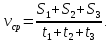
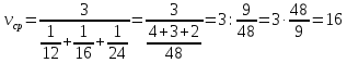
Например, если путь состоит из трех участков S₁, S₂, S₃, скорости, на которых были соответственно равны v₁, v₂, v₃, а время прохождения каждого участка соответственно t₁, t₂, t₃, то средняя скорость прохождения всех трех участков вычисляется по формуле:

Если путь поделен на равные части и известны скорости на каждом участке пути, то средняя скорость находится по формуле среднего гармонического. Например, средняя скорость движения на двух участках пути одинаковой длины вычисляется по формуле:

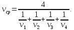
Средняя скорость движения на четырех участках одинаковой длины:

Если время движения поделено на равные части, то средняя скорость движения находится по формуле среднего арифметического. Например, если половину времени тело двигалось со скоростью , а вторую половину времени – со скоростью , то

Задача 1. Первые 190 км автомобиль ехал со скоростью 50 км/ч, следующие 180 км – со скоростью 90 км/ч, а затем 170 км – со скоростью 100 км/ч. Найдите среднюю скорость автомобиля на протяжении всего пути. Ответ дайте в км/ч.

Решение:

Занесем все исходные данные в таблицу (расстояния и скорости на каждом участке) и составим выражения для вычисления времени движения на каждом участке:

	Путь	Скорость	Время
1-й участок	190	50
2-й участок	180	90
3-й участок	170	100
Сумма	540

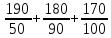
Чтобы найти среднюю скорость на протяжении пути, нужно весь путь разделить на все время движения. Средняя скорость автомобиля:

км/ч).

Ответ: 72 км/ч.

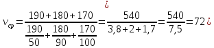
Задача 2. Первую треть трассы велосипедист ехал со скоростью 12 км/ч, вторую треть – со скоростью 16 км/ч, а последнюю треть – со скоростью 24 км/ч. Найдите среднюю скорость велосипедиста на протяжении всего пути.

Решение:

Способ 1.

Найдем среднюю скорость по формуле среднего гармонического:

(км/ч).

Способ 2.

Если забыли формулу среднего гармонического, то можно найти среднюю скорость по формуле:

Пусть S км – длина каждого участка трассы (можно принять длину каждого участка за 1).

	Путь	Скорость	Время
1-й участок	S	12
2-й участок	S	16
3-й участок	S	24
Сумма	3S

Получили: весь путь равен 3S км, время, потраченное на весь путь:

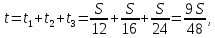
средняя скорость 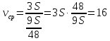(км/ч).

Ответ: 16 км/ч.

Задача 3. Автомобиль ехал первую половину пути со скоростью 40 км/ч, а вторую половину пути – со скоростью 60 км/ч. Найдите среднюю скорость движения автомобиля на всем пути. Ответ дайте в км/ч.

Решение:

Способ 1.

По формуле среднего гармонического

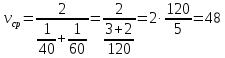(км/ч).

Способ 2.

Примем длину половины пути за 1. Тогда весь путь равен 1 + 1 = 2, все время движения: 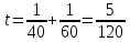, а средняя скорость

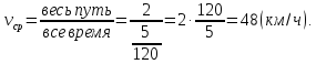
Ответ: 48 км/ч.

Задача 4. Путешественник переплыл океан на яхте со средней скоростью 30 км/ч. Обратно он летел на самолете со скоростью 570 км/ч. Найдите среднюю скорость путешественника на протяжении всего пути. Ответ дайте в км/ч.

Решение:

По формуле среднего гармонического

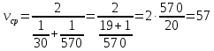(км/ч).

Ответ: 57 км/ч.

Задача 5. Автомобиль двигался половину времени со скоростью 80 км/ч, а вторую половину времени – со скоростью 100 км/ч. Найдите среднюю скорость автомобиля на всем пути. Ответ дайте в км/ч.

Решение:

Способ 1.

Найдем среднюю скорость по формуле среднего арифметического:

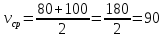(км/ч).

Способ 2.

Примем половину времени за 1.

	Скорость	Время	Путь
1-й участок	80	1
2-й участок	100	1
Сумма		2

Получили: весь путь равен 180 км, время, потраченное на весь путь равно 2. Значит, средняя скорость:

(км/ч).

Ответ: 90 км/ч.

Задачи для самостоятельного решения:

1. Первую треть трассы автомобиль ехал со скоростью 40 км/ч, вторую треть – со скоростью 60 км/ч, а последнюю – со скоростью 120 км/ч. Найдите среднюю скорость автомобиля на протяжении всего пути. Ответ дайте в км/ч.

2. Путешественник переплыл море на яхте со средней скоростью 21 км/ч. Обратно он летел на спортивном самолете со скоростью 420 км/ч. Найдите среднюю скорость путешественника на протяжении всего пути. Ответ дайте в км/ч.

3. Половину времени, затраченного на дорогу, автомобиль ехал со скоростью 74 км/ч, а вторую половину времени – со скоростью 66 км/ч. Найдите среднюю скорость автомобиля на протяжении всего пути. Ответ дайте в км/ч.

4. Первые два часа автомобиль ехал со скоростью 50 км/ч, следующий час – со скоростью 100 км/ч, а затем два часа – со скоростью 75 км/ч. Найдите среднюю скорость автомобиля на протяжении всего пути. Ответ дайте в км/ч.

5. Первый час автомобиль ехал со скоростью 100 км/ч, следующие два часа – со скоростью 90 км/ч, а затем два часа – со скоростью 80 км/ч. Найдите среднюю скорость автомобиля на протяжении всего пути. Ответ дайте в км/ч.

6. Первые 120 км автомобиль ехал со скоростью 60 км/ч, следующие 120 км — со скоростью 80 км/ч, а затем 150 км — со скоростью 100 км/ч. Найдите СК автомобиля на протяжении всего пути. Ответ дайте в км/ч.

Источник

Средняя
гармоническая. Эту среднюю называют
обратной средней арифметической,
поскольку эта величина используется
при k = -1.

Простая
средняя гармоническая используется
тогда, когда веса значений признака
одинаковы. Ее формулу можно вывести из
базовой формулы, подставив k = -1:

К
примеру, нам нужно вычислить среднюю
скорость двух автомашин, прошедших один
и тот же путь, но с разной скоростью:
первая — со скоростью 100 км/ч, вторая — 90
км/ч. Применяя метод средней гармонической,
мы вычисляем среднюю скорость:

В статистической практике чаще
используется гармоническая
взвешенная, формула которой имеет
вид

Данная
формула используется в тех случаях,
когда веса (или объемы явлений) по каждому
признаку не равны. В исходном соотношении
для расчета средней известен числитель,
но неизвестен знаменатель.

Например,
при расчете средней цены мы должны
пользоваться отношением суммы реализации
к количеству реализованных единиц. Нам
не известно количество реализованных
единиц (речь идет о разных товарах), но
известны суммы реализаций этих различных
товаров. Допустим, необходимо узнать
среднюю цену реализованных товаров:

Вид товара	Цена за единицу, руб.	Сумма реализаций, руб.
а	50	500
б	40	600
с	60	1200

Получаем

Если
здесь использовать формулу средней
арифметической, то можно получить
среднюю цену, которая будет нереальна.

16. Средняя геометрическая величина

Средняя геометрическая используется
для анализа динамики явлений и позволяет
определить средний коэффициент роста.
При расчете средней геометрической
индивидуальные значения признака
представляют собой относительные
показатели динамики, построенные в виде
цепных величин, как отношения каждого
уровня к предыдущему.

Средняя
геометрическая простая рассчитывается
по формуле:

Чаще
всего средняя геометрическая находит
свое применение при определении средних
темпов роста (средних коэффициентов
роста), когда индивидуальные значения
признака представлены в виде относительных
величин. Она используется также, если
необходимо найти среднюю между минимальным
и максимальным значениями признака
(например, между 100 и 1000000). Существуют
формулы для простой и взвешенной средней
геометрической.

17-18.
Медиана и мода — структурные
(распределительные) средние величины

Для
определения структуры совокупности
используют особые средние показатели,
к которым относятся медиана и мода, или
так называемые структурные средние.
Если средняя арифметическая рассчитывается
на основе использования всех вариантов
значений признака, то медиана и мода
характеризуют величину того варианта,
который занимает определенное среднее
положение в ранжированном вариационном
ряду.

Медиана (Ме) — это величина, которая
соответствует варианту, находящемуся
в середине ранжированного ряда.

Для ранжированного ряда с нечетным
числом индивидуальных величин (например,
1, 2, 3, 3, 6, 7, 9, 9, 10) медианой будет величина,
которая расположена в центре ряда, т.е.
пятая величина.

Для
ранжированного ряда с четным числом
индивидуальных величин (например, 1, 5,
7, 10, 11, 14) медианой будет средняя
арифметическая величина, которая
рассчитывается из двух смежных величин.
Для нашего случая медиана равна (7+10) :
2= 8,5.

То
есть для нахождения медианы сначала
необходимо определить ее порядковый
номер (ее положение в ранжированном
ряду) по формуле

где
n — число единиц в совокупности.

Численное
значение медианы определяют по накопленным
частотам в дискретном вариационном
ряду. Для этого сначала следует указать
интервал нахождения медианы в интервальном
ряду распределения. Медианным называют
первый интервал, где сумма накопленных
частот превышает половину наблюдений
от общего числа всех наблюдений.

Численное
значение медианы обычно определяют по
формуле

где
x_Ме — нижняя граница медианного
интервала; i — величина интервала; S_-1 —
накопленная частота интервала, которая
предшествует медианному; f — частота
медианного интервала.

Модой (Мо) называют значение
признака, которое встречается наиболее
часто у единиц совокупности. Для
дискретного ряда модой будет являться
вариант с наибольшей частотой. Для
определения моды интервального ряда
сначала определяют модальный интервал
(интервал, имеющий наибольшую частоту).
Затем в пределах этого интервала находят
то значение признака, которое может
являться модой.

Чтобы
найти конкретное значение моды, необходимо
использовать формулу

где
x_Мо — нижняя граница модального
интервала; i_Мо — величина
модального интервала; f_Мо —
частота модального интервала; f_Мо-1 —
частота интервала, предшествующего
модальному; f_Мо+1 — частота
интервала, следующего за модальным.

Мода
имеет широкое распространение в
маркетинговой деятельности при изучении
покупательского спроса, особенно при
определении пользующихся наибольшим
спросом размеров одежды и обуви, при
регулировании ценовой политики.

19-22.
Статистическая вариация, абсолютные и
относительные показатели вариации,
дисперсия и среднее квадратичное
отклонение

Вариа́ция —
различие значений какого-либо признака у
разных единиц совокупности за
один и тот же промежуток
времени. Причиной возникновения
вариации являются различные условия
существования разных единиц совокупности.
Вариация — необходимое условие
существования и развития массовых
явлений.^[1] Определение
вариации необходимо при
организации выборочного наблюдения, статистическом
моделировании и
планировании экспертных
опросов. По степени вариации
можно судить об однородности совокупности,
устойчивости значений признака,
типичности средней,
о взаимосвязи между какими-либо
признаками.

Для
измерения вариации признака используют
как абсолютные, так и относительные
показатели.

К абсолютным показателям
вариации относят: размах
вариации, среднее линейное отклонение,
среднее квадратическое отклонение,
дисперсию.

К относительным показателям
вариации относят: коэффициент
осцилляции, линейный коэффициент
вариации, относительное линейное
отклонение и др.

Размах
вариации R. Это самый доступный по
простоте расчета абсолютный показатель,
который определяется как разность между
самым большим и самым малым значениями
признака у единиц данной совокупности:

Размах вариации (размах колебаний)
— важный показатель колеблемости
признака, но он дает возможность увидеть
только крайние отклонения, что ограничивает
область его применения. Для более точной
характеристики вариации признака на
основе учета его колеблемости используются
другие показатели.

Среднее
линейное отклонение d, которое вычисляют
для того, чтобы учесть различия всех
единиц исследуемой совокупности. Эта
величина определяется как средняя
арифметическая из абсолютных значений
отклонений от средней. Так как сумма
отклонений значений признака от средней
величины равна нулю, то все отклонения
берутся по модулю.

Формула
среднего линейного отклонения (простая)

Формула
среднего линейного отклонения (взвешенная)

При использовании показателя среднего
линейного отклонения возникают
определенные неудобства, связанные с
тем, что приходится иметь дело не только
с положительными, но и с отрицательными
величинами, что побудило искать другие
способы оценки вариации, чтобы иметь
дело только с положительными величинами.
Таким способом стало возведение всех
отклонений во вторую степень. Обобщающие
показатели, найденные с использованием
вторых степеней отклонений, получили
очень широкое распространение. К таким
показателям относятся среднее
квадратическое отклонение и среднее
квадратическое отклонение в квадрате ,
которое называют дисперсией.

Средняя
квадратическая простая

Средняя
квадратическая взвешенная

Дисперсия есть
не что иное, как средний квадрат отклонений
индивидуальных значений признака от
его средней величины.

Формулы
дисперсии взвешенной и простой :

Расчет
дисперсии можно упростить. Для этого
используется способ отсчета от условного
нуля (способ моментов), если имеют
место равные интервалы в вариационном
ряду.

Кроме
показателей вариации, выраженных в
абсолютных величинах, в статистическом
исследовании используются показатели
вариации (V), выраженные в относительных
величинах, особенно для целей сравнения
колеблемости различных признаков одной
и той же совокупности или для сравнения
колеблемости одного и того же признака
в нескольких совокупностях.

Данные показатели рассчитываются как
отношение размаха вариации к средней
величине признака (коэффициент
осцилляции), отношение среднего
линейного отклонения к средней величине
признака (линейный коэффициент
вариации), отношение среднего
квадратического отклонения к средней
величине признака (коэффициент
вариации) и, как правило, выражаются
в процентах.

Формулы
расчета относительных показателей
вариации:

В
статистической практике наиболее часто
применяется коэффициент вариации. Он
используется не только для сравнительной
оценки вариации, но и для характеристики
однородности совокупности. Совокупность
считается однородной, если коэффициент
вариации не превышает 33% (для распределений,
близких к нормальному).

Виды
(показатели) дисперсий и правило их
сложения

В
статистическом исследовании очень
часто бывает необходимо не только
изучить вариации признака по всей
совокупности, но и проследить количественные
изменения признака по однородным группам
совокупности, а также и между группами.
Следовательно, помимо общей средней
для всей совокупности необходимо
просчитывать и частные средние величины
по отдельным группам.

Различают три вида дисперсий:

общая;
средняя
внутригрупповая;
межгрупповая.

Общая дисперсия характеризует
вариацию признака всей совокупности
под влиянием всех тех факторов, которые
обусловили данную вариацию.

Средняя
внутригрупповая дисперсия свидетельствует
о случайной вариации, которая может
возникнуть под влиянием каких-либо
неучтенных факторов и которая не зависит
от признака-фактора, положенного в
основу группировки. Данная дисперсия
рассчитывается следующим образом:
сначала рассчитываются дисперсии по
отдельным группам, затем рассчитывается
средняя внутригрупповая дисперсия.

Межгрупповая дисперсия (дисперсия
групповых средних) характеризует
систематическую вариацию, т.е. различия
в величине исследуемого признака,
возникающие под влиянием признака-фактора,
который положен в основу группировки.
Эта дисперсия рассчитывается по формуле

Все
три вида дисперсии связаны между собой:
общая дисперсия равна сумме средней
внутригрупповой дисперсии и межгрупповой
дисперсии:

Данное соотношение отражает закон,
который называют правилом сложения
дисперсий. Согласно этому закону
(правилу), общая дисперсия, которая
возникает под влиянием всех факторов,
равна сумме дисперсий, которые появляются
как под влиянием признака-фактора,
положенного в основу группировки, так
и под влиянием других факторов. Благодаря
правилу сложения дисперсий можно
определить, какая часть общей дисперсии
находится под влиянием признака-фактора,
положенного в основу группировки.

23-24.
Статистические методы изучения
взаимосвязи между явлениями. Виды связей

Важнейшей
целью статистики является изучение
объективно существующих связей между
явлениями. В ходе статистического
исследования этих связей необходимо
выявить причинно-следственные зависимости
между показателями, т.е. насколько
изменение одних показателей зависит
от изменения других показателей.

Существует
две категории зависимостей (функциональная
и корреляционная) и две группы признаков
(признаки-факторы и результативные
признаки). В отличие от функциональной
связи, где существует полное соответствие
между факторными и результативными
признаками, в корреляционной связи
отсутствует это полное соответствие.

Существует
два вида связи между факторами и
результативными признаками:

Соседние файлы в предмете [НЕСОРТИРОВАННОЕ]

Источник

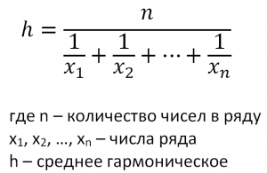
Среднее гармоническое

Среднее гармоническое — один из способов определения среднего значения числового ряда (наряду с медианой и средним арифметическим). Мы сделали калькулятор, который может рассчитать среднее гармоническое двух, трех — да любого количества чисел.

Рассчитывается среднее гармоническое по простой формуле и является обратной величиной к среднему от обратных к числам.

Среднее гармоническое удобно применять для решения задач, которые начинаются словами «первую половину пути автомобиль проехал со скоростью…». Например, первую половину пути автомобиль проехал со скоростью 60 км/ч вторую 90 км/ч. Найдите среднюю скорость. Просто введите в калькулятор два числа — 60 и 90 и получите ответ — 72 км/ч.

Калькулятор среднего гармонического

Как найти среднее гармоническое чисел

Лучше показать это на примере. Найдем среднее гармоническое двух чисел 1 и 2. Подставив значения в формулу получим такое выражение:

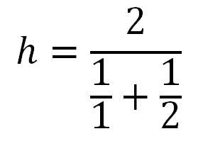
Здесь в числителе количество чисел (2), а в знаменателе сами числа. В результате расчета получаем, что среднее геометрическое чисел 1 и 2 равно 1,6666… или 1,(6).

Ваша оценка

[Оценок: 163 Средняя: 3.2]

Среднее гармоническое Автор admin средний рейтинг 3.2/5 — 163 рейтинги пользователей

Источник

Definition[edit]

Relationship with other means[edit]

Harmonic mean of two or three numbers[edit]

Two numbers[edit]

Three numbers[edit]

Weighted harmonic mean[edit]

Examples[edit]

In physics[edit]

Average speed[edit]

Density[edit]

Electricity[edit]

Optics[edit]

In finance[edit]

In geometry[edit]

In other sciences[edit]

Beta distribution[edit]

Lognormal distribution[edit]

Pareto distribution[edit]

Statistics[edit]

Sample distributions of mean and variance[edit]

Delta method[edit]

Jackknife method[edit]

Size biased sampling[edit]

Shifted variables[edit]

Moments[edit]

Sampling properties[edit]

Bias and variance estimators[edit]

Notes[edit]

See also[edit]

Notes[edit]

References[edit]

External links[edit]

16. Средняя геометрическая величина

Калькулятор среднего гармонического

Как найти среднее гармоническое чисел