Степени свободы (Df, C) – это количество параметров (точек контроля) Модели (Model). Они указывают количество независимых значений, которые могут изменяться в ходе анализа без нарушения каких-либо ограничений.
Пример.
- Рассмотрим Выборку (Sample) данных, состоящую для простоты из пяти положительных целых чисел. Значения могут быть любыми числами без известной связи между ними. Эта выборка данных теоретически должна иметь пять степеней свободы.
- Четыре числа в выборке — это {3, 8, 5 и 4}, а среднее значение всей выборки данных равно 6.
- Это должно означать, что пятое число равно 10. Иначе быть не может. У пятого значения нет свободы варьироваться.
- Таким образом, степень свободы для этой выборки данных равна 4.
Формула степени свободы выглядит следующим образом:
$$D_f = N — 1$$
где
D_f – степень свободы
N – количество значений
Математически степени свободы часто представляют, используя греческую букву «ню», которая выглядит так: ν. Вы наверняка встретите и такие сокращения: ‘d.o.f.’, ‘dof’, ‘d.f.’ или просто ‘df’.
Степени свободы в статистике
Степени свободы в статистике – это количество значений, используемых при вычислении переменной.
Степени свободы = Количество независимых значений — Количество статистик
Пример. У нас есть 50 независимых значений, и мы хотим вычислить одну-единственную статистику «среднее». Согласно формуле, степеней свободы будет 50 — 1 = 49.
Степени свободы в Машинном обучении
В прогностическом моделировании, степени свободы часто относятся к количеству параметров, включая данные, используемые при вычислении ошибки модели. Наилучший способ понять это – рассмотреть модель линейной регрессии.
Рассмотрим модель линейной регрессии для Датасета (Dataset) с двумя входными переменными. Нам потребуется один коэффициент в модели для каждой входной переменной, то есть модель будет иметь еще и два параметра.
$$hat{y} = x_1 * β_1 + x_2 * β_2$$
где
y – целевая переменная
x_1, x_2 – входные переменные
β_1, β_2 – параметры модели
Эта модель линейной регрессии имеет две степени свободы, потому что есть два параметра модели, которые должны быть оценены на основе обучающего датасета. Добавление еще одного столбца к данным (еще одной входной переменной) добавит модели еще одну степень свободы. Сложность обучения модели линейной регрессии описывается степенью свободы, например, «модель четвертой степени сложности» означает наличие четырех входных переменных, а также степень свободы, равную четырем.
Степени свободы для ошибки линейной регрессии
Количество обучающих примеров имеет значение и влияет на количество степеней свободы регрессионной модели. Представьте, что мы создаем модель линейной регрессии на базе датасета, состоящего из ста строк.
Сравнивая предсказания модели с реальными выходными значениями, мы минимизируем ошибку. Итоговая ошибка модели имеет одну степень свободы для каждого ряда за вычетом количества параметров. В нашем случае ошибка модели 98 степеней свободы (100 рядов — 2 параметра).
Итоговые степени свободы для линейной регрессии
Конечные степени свободы для модели линейной регрессии рассчитываются как сумма степеней свободы модели плюс степени свободы ошибки модели. В нашем примере это 100 (2 степени свободы модели + 98 степеней свободы ошибки). Как вы уже заметили, степеней свободы столько, сколько рядов в датасете.
Теперь рассмотрим набор данных из 100 строк, но теперь у нас есть 70 входных переменных. Это означает, что модель имеет еще и 70 коэффициентов, что дает нам d.o.f. ошибки, равной 30 (100 строк — 70 коэффициентов). d.o.f. самой модели по-прежнему равен ста.
Отрицательные степени свободы
Что происходит, когда у нас больше столбцов, чем строк данных? Отрицательные значения вполне допустимы здесь. Например, у нас может быть 100 строк данных и 10 000 переменных, к примеру, маркеры генов для 100 пациентов. Следовательно, модель линейной регрессии будет иметь 10 000 параметров, то есть модель будет иметь 10 000 степеней свободы.
Тогда степени свободы рассчитываются следующим образом:
Степень свободы модели = Количество независимых значение — Количество параметров = 100 — 10 000 = -9 900
В свою очередь, степени свободы модели линейной регрессии будут следующими:
Степени свободы модели линейной регрессии = Степени свободы модели — Степени свободы ошибки модели = 10 000 — 9 900 = 100
Фото: @mickeyoneil
Критерий Фишера и критерий Стьюдента в эконометрике
С помощью критерия Фишера оценивают качество регрессионной модели в целом и по параметрам.
Для этого выполняется сравнение полученного значения F и табличного F значения. F-критерия Фишера. F фактический определяется из отношения значений факторной и остаточной дисперсий, рассчитанных на одну степень свободы:

где n — число наблюдений;
m — число параметров при факторе х.
F табличный — это максимальное значение критерия под влиянием случайных факторов при текущих степенях свободы и уровне значимости а.
Уровень значимости а — вероятность не принять гипотезу при условии, что она верна. Как правило а принимается равной 0,05 или 0,01.
Если Fтабл > Fфакт то признается статистическая незначимость модели, ненадежность уравнения регрессии.
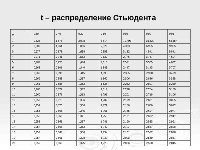
Таблицы по нахождению критерия Фишера и Стьюдента
Таблицы значений F-критерия Фишера и t-критерия Стьюдента Вы можете посмотреть здесь.
Табличное значение критерия Фишера вычисляют следующим образом:
- Определяют k1, которое равно количеству факторов (Х). Например, в однофакторной модели (модели парной регрессии) k1=1, в двухфакторной k=2.
- Определяют k2, которое определяется по формуле n — m — 1, где n — число наблюдений, m — количество факторов. Например, в однофакторной модели k2 = n — 2.
- На пересечении столбца k1 и строки k2 находят значение критерия Фишера
Для нахождения табличного значения критерия Стьюдента определяют число степеней свободы, которое определяется по формуле n — m — 1 и находят его значение при определенном уровне значимости (0,10, 0,05, 0,01).
Критерии Стьюдента
Для оценки статистической значимости модели по параметрам рассчитывают t-критерии Стьюдента.
Оценка значимости модели с помощью критерия Стьюдента проводится путем сравнения их значений с величиной случайной ошибки:

Случайные ошибки коэффициентов линейной регрессии и коэффициента корреляции определяются по формулам:

Сравнивая фактическое и табличное значения t-статистики и принимается или отвергается гипотеза о значимости модели по параметрам.
Зависимость между критерием Фишера и значением t-статистики Стьюдента определяется так

Как и в случае с оценкой значимости уравнения модели в целом, модель считается ненадежной если tтабл > tфакт
Видео лекциий по расчету критериев Фишера и Стьюдента
Для более подробного изучения расчетов критериев Фишера и Стьюдента советуем посмотреть это видео
Лекция 1. Критерии и Гипотезы
Лекция 2. Критерии и Гипотезы
Лекция 3. Критерии и Гипотезы
Определение доверительных интервалов
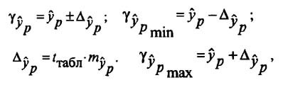
Для построения доверительного интервала определяется предельная ошибка А для обоих показателей:

Формулы для нахождения доверительных интервалов выглядят так

Прогнозное значение у определяется с помощью подстановки в
уравнение регрессии прогнозного значения х. Вычисляется средняя стандартная ошибка прогноза

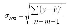
и находится доверительный интервал
Задача регрессионного анализа в предмете эконометрика состоит в анализе дисперсии изучаемого показателя y:

 общая сумма квадратов отклонений (TSS)
 сумма квадратов отклонений, обусловленная регрессией (RSS)
 остаточная сумма квадратов отклонений (ESS)
Долю дисперсии, обусловленную регрессией, в общей дисперсии показателя у характеризует коэффициент детерминации R, который должен превышать 50% (R2 > 0,5). В контрольных по эконометрике в ВУЗах этот показатель рассчитывается всегда.

Степени свободы в статистике
Уровень сложности
Простой
Время на прочтение
6 мин
Количество просмотров 1.6K

Автор статьи: Артем Михайлов
Статистический анализ играет важную роль в научных исследованиях, коммерческих деятельностях и в других областях. Однако, его результаты могут быть неточными, если не учитывать имеющиеся степени свободы. Степени свободы – это концепция, которая широко используется в статистике, и она позволяет более точно определить, насколько можно доверять полученным результатам.
В данной статье мы рассмотрим понятие степеней свободы, их роль в статистических расчетах, а также примеры их использования. Мы узнаем, как степени свободы помогают улучшить точность статистических выводов и в каких случаях их использование особенно важно.
Что такое степень свободы?
Степень свободы (Degree of Freedom, df) в статистике — это количество значений или наблюдений в выборке, которые могут быть изменены независимо друг от друга без изменения ее структуры. Можно сказать, что это количество переменных, которые оставляются свободными для варьирования после того, как структура выборки была определена.
Например, рассмотрим тест Стьюдента (t-Test), который используется для проверки гипотезы о равенстве средних значений двух выборок. В этом тесте степень свободы определяется как сумма степеней свободы двух выборок минус два (df = n1 + n2 — 2), где n1 и n2 — размеры выборок.
Чем больше степень свободы, тем меньше вероятность ложных выводов и тем более точными будут результаты теста. В случае же, если степень свободы будет низкой, то мы можем получить ложные результаты, так как мы не имеем достаточно информации для адекватной оценки статистических характеристик выборки.
Одним из важных факторов, влияющих на степень свободы, является размер выборки. Чем больше выборка, тем больше степень свободы, значит, чем больше выборка, тем менее вероятно получение ошибочных результатов в статистических тестах.
Также степень свободы важна при выборе статистической модели. К примеру, при построении линейной регрессии, степень свободы может использоваться для определения того, сколько переменных необходимо использовать в модели. Выбор модели слишком сложной или, наоборот, слишком простой (т.е. с недостаточной степенью свободы) может привести к неправильным выводам.
Таблица степеней свободы
Таблица степеней свободы – это таблица, которая заполняется в соответствии с типом и количеством переменных, которые используются в анализе статистических данных. Она используется для определения правильной формулы для расчета критических значений при проведении статистических тестов, таких как t-критерий, F-критерий и хи-квадрат тест.
В таблице степеней свободы могут быть два типа переменных: независимые (IV) и зависимые (DV). Количество степеней свободы для каждой переменной определяется путем вычитания единицы от общего количества наблюдений.
Для каждого теста, количество степеней свободы может быть разным в зависимости от характеристик выборки и типа теста. Например:
-
В t-критерии Стьюдента, количество степеней свободы зависит от размера выборки и количества групп, участвующих в сравнении. Если у нас есть две группы, количество степеней свободы будет равно n1+n2-2 (где n1 и n2 – это размер первой и второй групп соответственно).

-
В анализе дисперсии (ANOVA), количество степеней свободы будет зависеть от количества групп и количества элементов в каждой группе. Если есть количество групп (k) и общее количество элементов (N), то количество степеней свободы для межгрупповой дисперсии будет равно k-1, а для остаточной дисперсии будет равно N-k.
-
В хи-квадрат тесте, количество степеней свободы зависит от размера матрицы сопряженности. Если у нас есть матрица 2×2, то количество степеней свободы будет равно 1.
Таблица степеней свободы помогает убедиться, что мы используем правильные статистические формулы для расчетов, что позволяет получать более точные и надежные результаты при анализе статистических данных.
Примеры использования степеней свободы
Рассмотрим несколько практических примеров использования степеней свободы в статистике:
-
t-критерий Стьюдента. Это статистический тест, который используется для проверки значимости различия между средними двух независимых выборок. Для расчета t-критерия Стьюдента используется формула, которая включает в себя показатели меры центральной тенденции (среднее значение) и меры разброса (стандартное отклонение) для каждой выборки, а также степени свободы. В частности, степени свободы в расчете t-критерия Стьюдента определяются как сумма степеней свободы выборок, возведенная в степень двух, деленная на сумму квадратов степеней свободы выборок. Этот тест дает возможность оценить значимость различий между двумя выборками и узнать, велика ли вероятность случайного различия.

Предположим, что вы хотите определить, отличаются ли средние зарплаты мужчин и женщин в вашей компании. Вы можете использовать t-критерий для проверки этой гипотезы. Для этого вам нужно знать выборочные средние и стандартные отклонения для мужчин и женщин, а также общее число человек в каждой группе. После этого можно использовать формулу для расчета t-критерия, учитывая количество степеней свободы (количество людей в каждой группе минус 1).
-
Анализ дисперсии (ANOVA). Это статистический тест, который используется для сравнения средних значений нескольких групп. ANOVA расчитывается разнесением общего отклонения между группами на внутреннюю дисперсию (внутригрупповое отклонение) и межгрупповую дисперсию. Степени свободы в расчете ANOVA определяются как разность между общим числом наблюдений и числом использованных для расчета средних значений степеней свободы (то есть на 1 меньше числа групп). Внутригрупповые и межгрупповые степени свободы могут быть вычислены отдельно.

Предположим, что у вас есть несколько групп людей, проходящих тренировку для улучшения своего здоровья. Вы хотите определить, есть ли значимые различия в потере веса между этими группами. Для решения этого вопроса можно использовать ANOVA, для этого вам нужно знать выборочные средние и стандартные отклонения для каждой группы, а также общее количество участников в каждой группе. Затем используйте формулу для расчета F-критерия, учитывая количество степеней свободы, которое будет различаться в зависимости от количества групп и количества участников в каждой группе.
-
Хи-квадрат тест. Это статистический тест, в котором измеряется отклонение между фактическим и ожидаемым количеством наблюдений в наборе данных. Хи-квадрат тест может использоваться для проверки независимости двух переменных в категориальных данных, таких как таблицы сопряженности. Степени свободы в расчете Хи-квадрат теста определяются как разность между общим количеством наблюдений в таблице и количеством ограничений (то есть размерность таблицы минус 1, по каждому измерению). Если степени свободы достаточно высоки, то можно считать, что тест говорит о статистически значимых различиях между переменными.
Предположим, что у вас есть две переменных — пол (мужчина или женщина) и предпочитаемый вид спорта (баскетбол, футбол, хоккей и т.д.), и вы хотите проверить, есть ли статистически значимая связь между этими переменными. Для этого вы можете использовать хи-квадрат тест, для которого нужно разбить каждую категориальную переменную на несколько групп, затем измерить общее количество наблюдений в каждой ячейке таблицы. После того как вы подсчитаете значения статистики хи-квадрат, вы можете использовать таблицу степеней свободы, чтобы определить, является ли полученный результат значимым для определенного уровня доверия.
-
В корреляционном анализе, степени свободы используются для вычисления коэффициента корреляции между двумя переменными и определения статистической значимости этой связи. Обычно, чем больше степеней свободы, тем точнее оценки корреляции. Количество степеней свободы определяется как общее число наблюдений минус число неизвестных параметров.
Например, если мы исследуем связь между уровнем образования и доходом, то количество степеней свободы будет равно количеству наблюдений минус два, так как два параметра (уровень образования и доход) неизвестны.


Преимущества и недостатки
Преимущества использования степеней свободы в статистике включают следующее:
-
Корректность статистических тестов: использование степеней свободы позволяет правильно оценивать дисперсию и скорректировать стандартные ошибки. Это обеспечивает более точные тесты на статистическую значимость.
-
Увеличение мощности тестов: использование правильных степеней свободы может увеличить мощность статистических тестов. Это позволяет увидеть статистически значимые различия там, где их может не быть при использовании неправильных степеней свободы.
-
Более надежные выводы: правильное использование степеней свободы позволяет избежать ошибок первого и второго рода. Это позволяет давать более точные и надежные научные выводы.
Однако, использование степеней свободы также имеет некоторые ограничения:
-
Количество данных: необходимо иметь достаточно большое количество данных, чтобы определить степени свободы. В противном случае могут возникнуть ошибки в статистических тестах.
-
Некоторые статистические тесты зависят от предположений: некоторые статистические тесты, такие как t-тесты, предполагают нормальность распределения данных. Если данные не соответствуют этим предположениям, использование степеней свободы может привести к ошибкам.
-
Ошибки вязкости: иногда степени свободы могут быть неверными из-за ошибок в вычислениях. Это может привести к неправильным выводам из статистических тестов.
Заключение
Таким образом, степени свободы являются одним из ключевых параметров в статистических расчетах и оказывают большое влияние на результаты анализа данных. При этом, важно понимать, что оптимальное количество степеней свободы зависит от многих факторов, включая размер выборки и число независимых переменных. Поэтому, для правильного выбора количества степеней свободы, необходим обширный опыт в анализе данных и статистике.
Также следует отметить, что степени свободы являются только одним из аспектов статистического анализа, и их применение требует определенных знаний в области статистики.
Полезные рекомендации
Напоследок хочу порекомендовать несколько полезных бесплатных вебинаров от OTUS. Регистрация доступна по ссылкам ниже:
-
Построение архитектуры с иcпользованием облачных сервисов AWS
-
Профессия Системный Аналитик. Путь с нуля до Middle
-
Бережливое управление требованиями

Добавил:
Upload
Опубликованный материал нарушает ваши авторские права? Сообщите нам.
Вуз:
Предмет:
Файл:
Эконометрика, все лекции.doc
Скачиваний:
799
Добавлен:
01.06.2015
Размер:
3.64 Mб
Скачать
![]() (или
(или
распределение Пирсона) имеет
сумма квадратов n
независимых СВ
![]() (имеющих стандартное нормальное
(имеющих стандартное нормальное
распределение):![]() .
.
Стандартная
нормально распределенная СВ
![]() .
.
Число
степеней свободы СВ
![]()
равно n
.
Число
степеней свободы
![]() равно числу СВ, её составляющих,
равно числу СВ, её составляющих,
уменьшенному на число линейных связей
между ними.
![]()
определяется одним числом
![]() – числом степеней свободы (
– числом степеней свободы (![]() ).
).
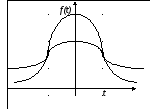
График
плотности вероятности СВ, имеющей
![]() —распределение
—распределение
лежит только в первой координатной
четверти и имеет асимметричный вид с
вытянутым правым «хвостом». Однако с
увеличением числа степеней свободы
распределение
![]()
приближается к нормальному.
|
|
Распределение |

4. Распределение Стьюдента(t – распределение)
Пусть
СВ
![]() ,
,
СВ![]() — независимая отZ
— независимая отZ
величина, имеющая распределение
![]() .
.
Тогда
величина
 имеетраспределение
Стьюдента (t
– распределение)
с n
степенями свободы (записывают T
~
![]() ).
).
Распределение
Стьюдента определяется только одним
параметром n
– числом степеней свободы.
|
|
График
При t |
5. Распределение Фишера (f – распределение)
|
Пусть
Тогда
имеет
Оно
При |
|


Таблица
критических значений t-критерия
Стьюдента
( Число степеней свободы)
|
|
Уровень |
|
Уровень |
||||||
|
0,1 |
0,05 |
0,01 |
0,001 |
0,1 |
0,05 |
0,01 |
0,001 |
||
|
1 |
6,314 |
12,71 |
63,657 |
636,62 |
23 |
1,714 |
2,069 |
2,807 |
3,768 |
|
2 |
2,920 |
4,303 |
9,925 |
31,599 |
24 |
1,711 |
2,064 |
2,797 |
3,745 |
|
3 |
2,353 |
3,182 |
5,841 |
12,924 |
25 |
1,708 |
2,060 |
2,787 |
3,725 |
|
4 |
2,132 |
2,776 |
4,604 |
8,610 |
26 |
1,706 |
2,056 |
2,779 |
3,707 |
|
5 |
2,015 |
2,571 |
4,032 |
6,869 |
27 |
1,703 |
2,052 |
2,771 |
3,690 |
|
6 |
1,943 |
2,447 |
3,707 |
5,959 |
28 |
1,701 |
2,048 |
2,763 |
3,674 |
|
7 |
1,895 |
2,365 |
3,499 |
5,408 |
29 |
1,699 |
2,045 |
2,756 |
3,656 |
|
8 |
1,860 |
2,306 |
3,355 |
5,040 |
30 |
1,697 |
2,042 |
2,750 |
3,646 |
|
9 |
1,833 |
2,262 |
3,250 |
4,781 |
35 |
1,689 |
2,031 |
2,726 |
3,598 |
|
10 |
1,812 |
2,228 |
3,169 |
4,587 |
40 |
1,684 |
2,021 |
2,704 |
3,554 |
|
11 |
1,796 |
2,201 |
3,106 |
4,437 |
45 |
1,680 |
2,014 |
2,690 |
3,527 |
|
12 |
1,782 |
2,179 |
3,055 |
4,318 |
50 |
1,676 |
2,009 |
2,678 |
3,505 |
|
13 |
1,771 |
2,160 |
3,012 |
4,221 |
60 |
1,670 |
2,000 |
2,660 |
3,505 |
|
14 |
1,761 |
2,145 |
2,977 |
4,140 |
70 |
1,664 |
1,994 |
2,649 |
3,458 |
|
15 |
1,753 |
2,131 |
2,947 |
4,073 |
80 |
1,662 |
1,990 |
2,639 |
3,416 |
|
16 |
1,746 |
2,120 |
2,921 |
4,015 |
90 |
1,661 |
1,987 |
2,632 |
3,402 |
|
17 |
1,740 |
2,110 |
2,898 |
3,965 |
100 |
1,660 |
1,984 |
2,626 |
3,391 |
|
18 |
1,734 |
2,101 |
2,878 |
3,922 |
120 |
1,658 |
1,980 |
2,617 |
3,373 |
|
19 |
1,729 |
2,093 |
2,861 |
3,883 |
150 |
1,656 |
1,978 |
2,612 |
3,359 |
|
20 |
1,725 |
2,086 |
2,845 |
3,850 |
200 |
1,653 |
1,972 |
2,501 |
3,340 |
|
21 |
1,721 |
2,080 |
2,831 |
3,819 |
500 |
1,648 |
1,965 |
2,586 |
3,210 |
|
22 |
1,717 |
2,074 |
2,819 |
3,792 |
|
1,645 |
1,960 |
2,580 |
3,291 |
Таблица
значений
![]() -критерия
-критерия
Фишера при уровне значимости![]()
|
|
1 |
2 |
3 |
4 |
5 |
6 |
8 |
12 |
24 |
|
|
1 |
161,5 |
199,5 |
215,7 |
224,6 |
230,2 |
233,9 |
238,9 |
243,9 |
249,0 |
254,3 |
|
2 |
18,51 |
19,00 |
19,16 |
19,25 |
19,30 |
19,33 |
19,37 |
19,41 |
19,45 |
19,50 |
|
3 |
10,13 |
9,55 |
9,28 |
9,12 |
9,01 |
8,94 |
8,84 |
8,74 |
8,64 |
8,53 |
|
4 |
7,71 |
6,94 |
6,59 |
6,39 |
6,26 |
6,16 |
6,04 |
5,91 |
5,77 |
5,63 |
|
5 |
6,61 |
5,79 |
5,41 |
5,19 |
5,05 |
4,95 |
4,82 |
4,68 |
4,53 |
4,36 |
|
6 |
5,99 |
5,14 |
4,76 |
4,53 |
4,39 |
4,28 |
4,15 |
4,00 |
3,84 |
3,67 |
|
7 |
5,59 |
4,74 |
4,35 |
4,12 |
3,97 |
3,87 |
3,73 |
3,57 |
3,41 |
3,23 |
|
8 |
5,32 |
4,46 |
4,07 |
3,84 |
3,69 |
3,58 |
3,44 |
3,28 |
3,12 |
2,93 |
|
9 |
5,12 |
4,26 |
3,86 |
3,63 |
3,48 |
3,37 |
3,23 |
3,07 |
2,90 |
2,71 |
|
10 |
4,96 |
4,10 |
3,71 |
3,48 |
3,33 |
3,22 |
3,07 |
2,91 |
2,74 |
2,54 |
|
11 |
4,84 |
3,98 |
3,59 |
3,36 |
3,20 |
3,09 |
2,95 |
2,79 |
2,61 |
2,40 |
|
12 |
4,75 |
3,88 |
3,49 |
3,26 |
3,11 |
3,00 |
2,85 |
2,69 |
2,50 |
2,30 |
|
13 |
4,67 |
3,80 |
3,41 |
3,18 |
3,02 |
2,92 |
2,77 |
2,60 |
2,42 |
2,21 |
|
14 |
4,60 |
3,74 |
3,34 |
3,11 |
2,96 |
2,85 |
2,70 |
2,53 |
2,35 |
2,13 |
|
15 |
4,54 |
3,68 |
3,29 |
3,06 |
2,90 |
2,79 |
2,64 |
2,48 |
2,29 |
2,07 |
|
16 |
4,49 |
3,63 |
3,24 |
3,01 |
2,85 |
2,74 |
2,59 |
2,42 |
2,24 |
2,01 |
|
17 |
4,45 |
3,59 |
3,20 |
2,96 |
2,81 |
2,70 |
2,55 |
2,38 |
2,19 |
1,96 |
|
18 |
4,41 |
3,55 |
3,16 |
2,93 |
2,77 |
2,66 |
2,51 |
2,34 |
2,15 |
1,92 |
|
19 |
4,38 |
3,52 |
3,13 |
2,90 |
2,74 |
2,63 |
2,48 |
2,31 |
2,11 |
1,88 |
|
20 |
4,35 |
3,49 |
3,10 |
2,87 |
2,71 |
2,60 |
2,45 |
2,28 |
2,08 |
1,84 |
|
21 |
4,32 |
3,47 |
3,07 |
2,84 |
2,68 |
2,57 |
2,42 |
2,25 |
2,05 |
1,81 |
|
22 |
4,30 |
3,44 |
3,05 |
2,82 |
2,66 |
2,55 |
2,40 |
2,23 |
2,03 |
1,78 |
|
23 |
4,28 |
3,42 |
3,03 |
2,80 |
2,64 |
2,53 |
2,38 |
2,20 |
2,00 |
1,76 |
|
24 |
4,26 |
3,40 |
3,01 |
2,78 |
2,62 |
2,51 |
2,36 |
2,18 |
1,98 |
1,73 |
|
25 |
4,24 |
3,38 |
2,99 |
2,76 |
2,60 |
2,49 |
2,34 |
2,16 |
1,96 |
1,71 |
|
26 |
4,22 |
3,37 |
2,98 |
2,74 |
2,59 |
2,47 |
2,32 |
2,15 |
1,95 |
1,69 |
|
27 |
4,21 |
3,35 |
2,96 |
2,73 |
2,57 |
2,46 |
2,30 |
2,13 |
1,93 |
1,67 |
|
28 |
4,20 |
3,34 |
2,95 |
2,71 |
2,56 |
2,44 |
2,29 |
2,12 |
1,91 |
1,65 |
|
29 |
4,18 |
3,33 |
2,93 |
2,70 |
2,54 |
2,43 |
2,28 |
2,10 |
1,90 |
1,64 |
|
30 |
4,17 |
3,32 |
2,92 |
2,69 |
2,53 |
2,42 |
2,27 |
2,09 |
1,89 |
1,62 |
|
35 |
4,12 |
3,26 |
2,87 |
2,64 |
2,48 |
2,37 |
2,22 |
2,04 |
1,83 |
1,57 |
|
40 |
4,08 |
3,23 |
2,84 |
2,61 |
2,45 |
2,34 |
2,18 |
2,00 |
1,79 |
1,51 |
|
45 |
4,06 |
3,21 |
2,81 |
2,58 |
2,42 |
2,31 |
2,15 |
1,97 |
1,76 |
1,48 |
|
50 |
4,03 |
3,18 |
2,79 |
2,56 |
2,40 |
2,29 |
2,13 |
1,95 |
1,74 |
1,44 |
|
60 |
4,00 |
3,15 |
2,76 |
2,52 |
2,37 |
2,25 |
2,10 |
1,92 |
1,70 |
1,39 |
|
70 |
3,98 |
3,13 |
2,74 |
2,50 |
2,35 |
2,23 |
2,07 |
1,89 |
1,67 |
1,35 |
|
80 |
3,96 |
3,11 |
2,72 |
2,49 |
2,33 |
2,21 |
2,06 |
1,88 |
1,65 |
1,31 |
|
90 |
3,95 |
3,10 |
2,71 |
2,47 |
2,32 |
2,20 |
2,04 |
1,86 |
1,64 |
1,28 |
|
100 |
3,94 |
3,09 |
2,70 |
2,46 |
2,30 |
2,19 |
2,03 |
1,85 |
1,63 |
1,26 |
|
125 |
3,92 |
3,07 |
2,68 |
2,44 |
2,29 |
2,17 |
2,01 |
1,83 |
1,60 |
1,21 |
|
150 |
3,90 |
3,06 |
2,66 |
2,43 |
2,27 |
2,16 |
2,00 |
1,82 |
1,59 |
1,18 |
|
200 |
3,89 |
3,04 |
2,65 |
2,42 |
2,26 |
2,14 |
1,98 |
1,80 |
1,57 |
1,14 |
|
300 |
3,87 |
3,03 |
2,64 |
2,41 |
2,25 |
2,13 |
1,97 |
1,79 |
1,55 |
1,10 |
|
400 |
3,86 |
3,02 |
2,63 |
2,40 |
2,24 |
2,12 |
1,96 |
1,78 |
1,54 |
1,07 |
|
500 |
3,86 |
3,01 |
2,62 |
2,39 |
2,23 |
2,11 |
1,96 |
1,77 |
1,54 |
1,06 |
|
1000 |
3,85 |
3,00 |
2,61 |
2,38 |
2,22 |
2,10 |
1,95 |
1,76 |
1,53 |
1,03 |
|
|
3,84 |
2,99 |
2,60 |
2,37 |
2,21 |
2,09 |
1,94 |
1,75 |
1,52 |
1 |
Соседние файлы в предмете [НЕСОРТИРОВАННОЕ]
- #
- #
- #
- #
- #
- #
- #
- #
- #
- #
- #
In statistics, the number of degrees of freedom is the number of values in the final calculation of a statistic that are free to vary.[1]
Estimates of statistical parameters can be based upon different amounts of information or data. The number of independent pieces of information that go into the estimate of a parameter is called the degrees of freedom. In general, the degrees of freedom of an estimate of a parameter are equal to the number of independent scores that go into the estimate minus the number of parameters used as intermediate steps in the estimation of the parameter itself. For example, if the variance is to be estimated from a random sample of N independent scores, then the degrees of freedom is equal to the number of independent scores (N) minus the number of parameters estimated as intermediate steps (one, namely, the sample mean) and is therefore equal to N − 1.[2]
Mathematically, degrees of freedom is the number of dimensions of the domain of a random vector, or essentially the number of «free» components (how many components need to be known before the vector is fully determined).
The term is most often used in the context of linear models (linear regression, analysis of variance), where certain random vectors are constrained to lie in linear subspaces, and the number of degrees of freedom is the dimension of the subspace. The degrees of freedom are also commonly associated with the squared lengths (or «sum of squares» of the coordinates) of such vectors, and the parameters of chi-squared and other distributions that arise in associated statistical testing problems.
While introductory textbooks may introduce degrees of freedom as distribution parameters or through hypothesis testing, it is the underlying geometry that defines degrees of freedom, and is critical to a proper understanding of the concept.
History[edit]
Although the basic concept of degrees of freedom was recognized as early as 1821 in the work of German astronomer and mathematician Carl Friedrich Gauss,[3] its modern definition and usage was first elaborated by English statistician William Sealy Gosset in his 1908 Biometrika article «The Probable Error of a Mean», published under the pen name «Student».[4] While Gosset did not actually use the term ‘degrees of freedom’, he explained the concept in the course of developing what became known as Student’s t-distribution. The term itself was popularized by English statistician and biologist Ronald Fisher, beginning with his 1922 work on chi squares.[5]
Notation[edit]
In equations, the typical symbol for degrees of freedom is ν (lowercase Greek letter nu). In text and tables, the abbreviation «d.f.» is commonly used. R. A. Fisher used n to symbolize degrees of freedom but modern usage typically reserves n for sample size.
Of random vectors[edit]
Geometrically, the degrees of freedom can be interpreted as the dimension of certain vector subspaces. As a starting point, suppose that we have a sample of independent normally distributed observations,

This can be represented as an n-dimensional random vector:

Since this random vector can lie anywhere in n-dimensional space, it has n degrees of freedom.
Now, let  be the sample mean. The random vector can be decomposed as the sum of the sample mean plus a vector of residuals:

The first vector on the right-hand side is constrained to be a multiple of the vector of 1’s, and the only free quantity is . It therefore has 1 degree of freedom.
The second vector is constrained by the relation  . The first n − 1 components of this vector can be anything. However, once you know the first n − 1 components, the constraint tells you the value of the nth component. Therefore, this vector has n − 1 degrees of freedom.
Mathematically, the first vector is the Oblique projection of the data vector onto the subspace spanned by the vector of 1’s. The 1 degree of freedom is the dimension of this subspace. The second residual vector is the least-squares projection onto the (n − 1)-dimensional orthogonal complement of this subspace, and has n − 1 degrees of freedom.
In statistical testing applications, often one is not directly interested in the component vectors, but rather in their squared lengths. In the example above, the residual sum-of-squares is

If the data points  are normally distributed with mean 0 and variance
  , then the residual sum of squares has a scaled chi-squared distribution (scaled by the factor ), with n − 1 degrees of freedom. The degrees-of-freedom, here a parameter of the distribution, can still be interpreted as the dimension of an underlying vector subspace.
Likewise, the one-sample t-test statistic,

follows a Student’s t distribution with n − 1 degrees of freedom when the hypothesized mean  is correct. Again, the degrees-of-freedom arises from the residual vector in the denominator.
In structural equation models[edit]
When the results of structural equation models (SEM) are presented, they generally include one or more indices of overall model fit, the most common of which is a χ2 statistic. This forms the basis for other indices that are commonly reported. Although it is these other statistics that are most commonly interpreted, the degrees of freedom of the χ2 are essential to understanding model fit as well as the nature of the model itself.
Degrees of freedom in SEM are computed as a difference between the number of unique pieces of information that are used as input into the analysis, sometimes called knowns, and the number of parameters that are uniquely estimated, sometimes called unknowns. For example, in a one-factor confirmatory factor analysis with 4 items, there are 10 knowns (the six unique covariances among the four items and the four item variances) and 8 unknowns (4 factor loadings and 4 error variances) for 2 degrees of freedom. Degrees of freedom are important to the understanding of model fit if for no other reason than that, all else being equal, the fewer degrees of freedom, the better indices such as χ2 will be.
It has been shown that degrees of freedom can be used by readers of papers that contain SEMs to determine if the authors of those papers are in fact reporting the correct model fit statistics. In the organizational sciences, for example, nearly half of papers published in top journals report degrees of freedom that are inconsistent with the models described in those papers, leaving the reader to wonder which models were actually tested.[6]
Of residuals[edit]
A common way to think of degrees of freedom is as the number of independent pieces of information available to estimate another piece of information. More concretely, the number of degrees of freedom is the number of independent observations in a sample of data that are available to estimate a parameter of the population from which that sample is drawn. For example, if we have two observations, when calculating the mean we have two independent observations; however, when calculating the variance, we have only one independent observation, since the two observations are equally distant from the sample mean.
In fitting statistical models to data, the vectors of residuals are constrained to lie in a space of smaller dimension than the number of components in the vector. That smaller dimension is the number of degrees of freedom for error, also called residual degrees of freedom.
Example[edit]
Perhaps the simplest example is this. Suppose

are random variables each with expected value μ, and let

be the «sample mean.» Then the quantities

are residuals that may be considered estimates of the errors Xi − μ. The sum of the residuals (unlike the sum of the errors) is necessarily 0. If one knows the values of any n − 1 of the residuals, one can thus find the last one. That means they are constrained to lie in a space of dimension n − 1. One says that there are n − 1 degrees of freedom for errors.
An example which is only slightly less simple is that of least squares estimation of a and b in the model

where xi is given, but ei and hence Yi are random. Let  and
and  be the least-squares estimates of a and b. Then the residuals

are constrained to lie within the space defined by the two equations


One says that there are n − 2 degrees of freedom for error.
Notationally, the capital letter Y is used in specifying the model, while lower-case y in the definition of the residuals; that is because the former are hypothesized random variables and the latter are actual data.
We can generalise this to multiple regression involving p parameters and covariates (e.g. p − 1 predictors and one mean (=intercept in the regression)), in which case the cost in degrees of freedom of the fit is p, leaving n — p degrees of freedom for errors
In linear models[edit]
The demonstration of the t and chi-squared distributions for one-sample problems above is the simplest example where degrees-of-freedom arise. However, similar geometry and vector decompositions underlie much of the theory of linear models, including linear regression and analysis of variance. An explicit example based on comparison of three means is presented here; the geometry of linear models is discussed in more complete detail by Christensen (2002).[7]
Suppose independent observations are made for three populations,  ,
,  and
and  . The restriction to three groups and equal sample sizes simplifies notation, but the ideas are easily generalized.
The observations can be decomposed as

where  are the means of the individual samples, and
 is the mean of all 3n observations. In vector notation this decomposition can be written as

The observation vector, on the left-hand side, has 3n degrees of freedom. On the right-hand side, the first vector has one degree of freedom (or dimension) for the overall mean. The second vector depends on three random variables,  ,
,  and
and  . However, these must sum to 0 and so are constrained; the vector therefore must lie in a 2-dimensional subspace, and has 2 degrees of freedom. The remaining 3n − 3 degrees of freedom are in the residual vector (made up of n − 1 degrees of freedom within each of the populations).
In analysis of variance (ANOVA)[edit]
In statistical testing problems, one usually is not interested in the component vectors themselves, but rather in their squared lengths, or Sum of Squares. The degrees of freedom associated with a sum-of-squares is the degrees-of-freedom of the corresponding component vectors.
The three-population example above is an example of one-way Analysis of Variance. The model, or treatment, sum-of-squares is the squared length of the second vector,

with 2 degrees of freedom. The residual, or error, sum-of-squares is

with 3(n−1) degrees of freedom. Of course, introductory books on ANOVA usually state formulae without showing the vectors, but it is this underlying geometry that gives rise to SS formulae, and shows how to unambiguously determine the degrees of freedom in any given situation.
Under the null hypothesis of no difference between population means (and assuming that standard ANOVA regularity assumptions are satisfied) the sums of squares have scaled chi-squared distributions, with the corresponding degrees of freedom. The F-test statistic is the ratio, after scaling by the degrees of freedom. If there is no difference between population means this ratio follows an F-distribution with 2 and 3n − 3 degrees of freedom.
In some complicated settings, such as unbalanced split-plot designs, the sums-of-squares no longer have scaled chi-squared distributions. Comparison of sum-of-squares with degrees-of-freedom is no longer meaningful, and software may report certain fractional ‘degrees of freedom’ in these cases. Such numbers have no genuine degrees-of-freedom interpretation, but are simply providing an approximate chi-squared distribution for the corresponding sum-of-squares. The details of such approximations are beyond the scope of this page.
In probability distributions[edit]
Several commonly encountered statistical distributions (Student’s t, chi-squared, F) have parameters that are commonly referred to as degrees of freedom. This terminology simply reflects that in many applications where these distributions occur, the parameter corresponds to the degrees of freedom of an underlying random vector, as in the preceding ANOVA example. Another simple example is: if  are independent normal
  random variables, the statistic

follows a chi-squared distribution with n − 1 degrees of freedom. Here, the degrees of freedom arises from the residual sum-of-squares in the numerator, and in turn the n − 1 degrees of freedom of the underlying residual vector  .
.
In the application of these distributions to linear models, the degrees of freedom parameters can take only integer values. The underlying families of distributions allow fractional values for the degrees-of-freedom parameters, which can arise in more sophisticated uses. One set of examples is problems where chi-squared approximations based on effective degrees of freedom are used. In other applications, such as modelling heavy-tailed data, a t or F-distribution may be used as an empirical model. In these cases, there is no particular degrees of freedom interpretation to the distribution parameters, even though the terminology may continue to be used.
In non-standard regression[edit]
Many non-standard regression methods, including regularized least squares (e.g., ridge regression), linear smoothers, smoothing splines, and semiparametric regression are not based on ordinary least squares projections, but rather on regularized (generalized and/or penalized) least-squares, and so degrees of freedom defined in terms of dimensionality is generally not useful for these procedures. However, these procedures are still linear in the observations, and the fitted values of the regression can be expressed in the form

where  is the vector of fitted values at each of the original covariate values from the fitted model, y is the original vector of responses, and H is the hat matrix or, more generally, smoother matrix.
For statistical inference, sums-of-squares can still be formed: the model sum-of-squares is  ; the residual sum-of-squares is
  . However, because H does not correspond to an ordinary least-squares fit (i.e. is not an orthogonal projection), these sums-of-squares no longer have (scaled, non-central) chi-squared distributions, and dimensionally defined degrees-of-freedom are not useful.
The effective degrees of freedom of the fit can be defined in various ways to implement goodness-of-fit tests, cross-validation, and other statistical inference procedures. Here one can distinguish between regression effective degrees of freedom and residual effective degrees of freedom.
Regression effective degrees of freedom[edit]
For the regression effective degrees of freedom, appropriate definitions can include the trace of the hat matrix,[8] tr(H), the trace of the quadratic form of the hat matrix, tr(H’H), the form tr(2H – H H’), or the Satterthwaite approximation, tr(H’H)2/tr(H’HH’H).[9]
In the case of linear regression, the hat matrix H is X(X ‘X)−1X ‘, and all these definitions reduce to the usual degrees of freedom. Notice that

the regression (not residual) degrees of freedom in linear models are «the sum of the sensitivities of the fitted values with respect to the observed response values»,[10] i.e. the sum of leverage scores.
One way to help to conceptualize this is to consider a simple smoothing matrix like a Gaussian blur, used to mitigate data noise. In contrast to a simple linear or polynomial fit, computing the effective degrees of freedom of the smoothing function is not straight-forward. In these cases, it is important to estimate the Degrees of Freedom permitted by the  matrix so that the residual degrees of freedom can then be used to estimate statistical tests such as
  .
.
Residual effective degrees of freedom[edit]
There are corresponding definitions of residual effective degrees-of-freedom (redf), with H replaced by I − H. For example, if the goal is to estimate error variance, the redf would be defined as tr((I − H)'(I − H)), and the unbiased estimate is (with  ),
),

or:[11][12][13][14]


The last approximation above[12] reduces the computational cost from O(n2) to only O(n). In general the numerator would be the objective function being minimized; e.g., if the hat matrix includes an observation covariance matrix, Σ, then  becomes
  .
.
General[edit]
Note that unlike in the original case, non-integer degrees of freedom are allowed, though the value must usually still be constrained between 0 and n.[15]
Consider, as an example, the k-nearest neighbour smoother, which is the average of the k nearest measured values to the given point. Then, at each of the n measured points, the weight of the original value on the linear combination that makes up the predicted value is just 1/k. Thus, the trace of the hat matrix is n/k. Thus the smooth costs n/k effective degrees of freedom.
As another example, consider the existence of nearly duplicated observations. Naive application of classical formula, n − p, would lead to over-estimation of the residuals degree of freedom, as if each observation were independent. More realistically, though, the hat matrix H = X(X ‘ Σ−1 X)−1X ‘ Σ−1 would involve an observation covariance matrix Σ indicating the non-zero correlation among observations.
The more general formulation of effective degree of freedom would result in a more realistic estimate for, e.g., the error variance σ2, which in its turn scales the unknown parameters’ a posteriori standard deviation; the degree of freedom will also affect the expansion factor necessary to produce an error ellipse for a given confidence level.
Other formulations[edit]
Similar concepts are the equivalent degrees of freedom in non-parametric regression,[16] the degree of freedom of signal in atmospheric studies,[17][18] and the non-integer degree of freedom in geodesy.[19][20]
The residual sum-of-squares has a generalized chi-squared distribution, and the theory associated with this distribution[21] provides an alternative route to the answers provided above.[further explanation needed]
See also[edit]
- Bessel’s correction
- Chi-squared per degree of freedom
- Pooled degrees of freedom
- Replication (statistics)
- Sample size
- Statistical model
- Variance
References[edit]
- ^ «Degrees of Freedom». Glossary of Statistical Terms. Animated Software. Retrieved 2008-08-21.
- ^ Lane, David M. «Degrees of Freedom». HyperStat Online. Statistics Solutions. Retrieved 2008-08-21.
- ^ Walker, H. M. (April 1940). «Degrees of Freedom» (PDF). Journal of Educational Psychology. 31 (4): 253–269. doi:10.1037/h0054588.
- ^ Student (March 1908). «The Probable Error of a Mean». Biometrika. 6 (1): 1–25. doi:10.2307/2331554. JSTOR 2331554.
- ^ Fisher, R. A. (January 1922). «On the Interpretation of χ2 from Contingency Tables, and the Calculation of P». Journal of the Royal Statistical Society. 85 (1): 87–94. doi:10.2307/2340521. JSTOR 2340521.
- ^ Cortina, J. M., Green, J. P., Keeler, K. R., & Vandenberg, R. J. (2017). Degrees of freedom in SEM: Are we testing the models that we claim to test?. Organizational Research Methods, 20(3), 350-378.
- ^ Christensen, Ronald (2002). Plane Answers to Complex Questions: The Theory of Linear Models (Third ed.). New York: Springer. ISBN 0-387-95361-2.
- ^ Trevor Hastie, Robert Tibshirani, Jerome H. Friedman (2009), The elements of statistical learning: data mining, inference, and prediction, 2nd ed., 746 p. ISBN 978-0-387-84857-0, doi:10.1007/978-0-387-84858-7, [1] (eq.(5.16))
- ^ Fox, J.; Sage Publications, inc; SAGE. (2000). Nonparametric Simple Regression: Smoothing Scatterplots. Nonparametric Simple Regression: Smoothing Scatterplots. SAGE Publications. p. 58. ISBN 978-0-7619-1585-0. Retrieved 2020-08-28.
- ^ Ye, J. (1998), «On Measuring and Correcting the Effects of Data Mining and Model Selection», Journal of the American Statistical Association, 93 (441), 120–131. JSTOR 2669609 (eq.(7))
- ^ Clive Loader (1999), Local regression and likelihood, ISBN 978-0-387-98775-0, doi:10.1007/b98858, (eq.(2.18), p. 30)
- ^ a b Trevor Hastie, Robert Tibshirani (1990), Generalized additive models, CRC Press, (p. 54) and (eq.(B.1), p. 305))
- ^ Simon N. Wood (2006), Generalized additive models: an introduction with R, CRC Press, (eq.(4,14), p. 172)
- ^ David Ruppert, M. P. Wand, R. J. Carroll (2003), Semiparametric Regression, Cambridge University Press (eq.(3.28), p. 82)
- ^ James S. Hodges (2014) Richly Parameterized Linear Models, CRC Press. [2]
- ^ Peter J. Green, B. W. Silverman (1994), Nonparametric regression and generalized linear models: a roughness penalty approach, CRC Press (eq.(3.15), p. 37)
- ^ Clive D. Rodgers (2000), Inverse methods for atmospheric sounding: theory and practice, World Scientific (eq.(2.56), p. 31)
- ^ Adrian Doicu, Thomas Trautmann, Franz Schreier (2010), Numerical Regularization for Atmospheric Inverse Problems, Springer (eq.(4.26), p. 114)
- ^ D. Dong, T. A. Herring and R. W. King (1997), Estimating regional deformation from a combination of space and terrestrial geodetic data, J. Geodesy, 72 (4), 200–214, doi:10.1007/s001900050161 (eq.(27), p. 205)
- ^ H. Theil (1963), «On the Use of Incomplete Prior Information in Regression Analysis», Journal of the American Statistical Association, 58 (302), 401–414 JSTOR 2283275 (eq.(5.19)–(5.20))
- ^ Jones, D.A. (1983) «Statistical analysis of empirical models fitted by optimisation», Biometrika, 70 (1), 67–88
Further reading[edit]
- Bowers, David (1982). Statistics for Economists. London: Macmillan. pp. 175–178. ISBN 0-333-30110-2.
- Eisenhauer, J. G. (2008). «Degrees of Freedom». Teaching Statistics. 30 (3): 75–78. doi:10.1111/j.1467-9639.2008.00324.x. S2CID 121982952.
- Good, I. J. (1973). «What Are Degrees of Freedom?». The American Statistician. 27 (5): 227–228. doi:10.1080/00031305.1973.10479042. JSTOR 3087407.
- Walker, H. W. (1940). «Degrees of Freedom». Journal of Educational Psychology. 31 (4): 253–269. doi:10.1037/h0054588. Transcription by C Olsen with errata
External links[edit]
- Yu, Chong-ho (1997) Illustrating degrees of freedom in terms of sample size and dimensionality
- Dallal, GE. (2003) Degrees of Freedom