Как найти суммарную скорость

Закон сложения скоростей — что это такое

В классической механике применяют термин, который звучит, как абсолютная скорость точки. Данная величина является суммой двух векторов: относительная и переносная скорости точки. В подобном равенстве выражена теорема сложения скоростей. Общепринятым положением является равенство скорости движения какого-либо объекта в рамках неподвижной системы отсчета и векторной суммы скорости аналогичного физического тела в условиях относительно подвижной системы отсчета. Данными координатами определяется непосредственное нахождение тела.

Классический вид, формула расчета

Релятивистским законом сложения скоростей являются соотношения, справедливые для частицы, перемещающейся параллельно относительной скорости систем отсчета:

Осторожно! Если преподаватель обнаружит плагиат в работе, не избежать крупных проблем (вплоть до отчисления). Если нет возможности написать самому, закажите тут.

(К) и (K^{,})

Соотношение теории имеет следующий вид:

(u_{x}=frac{u_{x}^{,}+upsilon }{1+frac{upsilon }{c^{2}}u^{,}_{x}})

(u_{y}=0)

(u_{z}=0)

В случае, когда u<<с, наблюдают переход релятивистских формул в формулы, характерные для классической механики:

(u_{x}=u^{,}_{x}+upsilon)

(u_{y}=0)

(u_{z}=0)

Преобразование координат и времени

Закон сложения скоростей вытекает из физических процессов. Представленное выше соотношение получено в результате преобразований координат и времени. Можно представить частицу, которая в определенное время (t^{,}) зафиксирована в точке с координатами: (x^{,}), (y^{,}), (z^{,}).

Спустя какой-то небольшой промежуток времени (Delta t^{,}) частица переместилась в точку:

(x^{,}+Delta x^{,})

(y^{,}+Delta y^{,})

(z^{,}+Delta z^{,})

В системе отсчета (K^{,}).

Таким образом, при движении частицы происходят два события. Можно записать следующую формулу:

(Delta x^{,}=Delta v^{,}_{x}Delta t^{,})

где ( Delta v^{,}_{x}) представляет собой х компоненту скорости частицы в системе (K^{,}.)

Такие же равенства можно вычислить относительно других компонент. Аналогично координатам преобразуются разности координат и промежутки времени (Delta x), (Delta y), (Delta z). (Delta t).

Уравнения будут иметь следующий вид:

(Delta x=Delta x^{,}+VDelta t^{,})

(Delta y=Delta y^{,})

(Delta z=Delta z^{,})

(Delta t=Delta t^{,})

Исходя из составленных формул можно сделать вывод о том, что компоненты скорости той же частицы в системе (К) будут записаны следующим образом:

(upsilon _{x}=frac{Delta x}{Delta t}=frac{left(Delta x^{,}+VDelta t^{,} right)}{Delta t}=upsilon _{x}^{,} +V)

(upsilon _{y}=upsilon _{y}^{,})

(upsilon _{z}=upsilon _{z}^{,})

Уравнение представляет собой закон сложения скоростей. Данную закономерность можно привести в векторный вид:

(vec{upsilon }=vec{upsilon ^{,}}+V)

Координаты в системе (К) и системе (K^{,}) будут параллельны.

Алгоритм решения задач

Существуют правила, которые являются основой механической физики. Исходя из данных соотношений, можно рассмотреть примеры сложения скоростей. Простейшими объектами для объяснения физических законов являются, к примеру, человек и любой перемещающийся в пространстве объект, с которым он прямо или косвенно взаимодействует.

Пример

Можно представить, что человек совершает прямолинейное движение вдоль коридора пассажирского поезда со скоростью пять километров в час. При этом равномерная скорость состава составляет 100 километров в час. Скорость человека, относительно пространства, которое его окружает, будет равна 105 километрам в час. Следует учитывать одинаковое направление перемещения человека и поезда.

В случае, когда направления движения человека и транспорта противоположны, данный принцип также справедлив. Тогда человек будет двигаться относительно окружающего пространства со скоростью 95 километров в час.

При рассмотрении объектов, скорости которых равны, можно сделать вывод, что относительно друг друга они неподвижны. Во время вращения скорость рассматриваемого тела представляет собой совокупность скоростей перемещения тела относительно движущейся поверхности другого объекта.

Решение задач на сложение скоростей выполняется в несколько этапов:

1. Следует начать с выбора тела отсчета, которое связано с неподвижной системой координат.
2. Далее необходимо определить тело отсчета, которое совершает движение по отношению к первому телу, и связать его с подвижной системой координат.
3. Изучение движения тела в двух координатных системах.
4. Запись закона сложения скоростей, относительно конкретных условий задачи.

Задача 1

На примере рассмотрено равномерное движение двух поездов друг за другом. Первый поезд перемещается со скоростью 80 км/ч, а второй — 60 км/ч. Требуется рассчитать, какова скорость второго поезда относительно первого.

Решение

Следует обозначить скорость первого транспортного средства по отношению к земле с помощью (vec{v_{1}}.)

Тогда скорость  второго поезда составит (vec{v_{2}}.)

Исходя из закона сложения скоростей:

(vec{v_{2}}=vec{v_{2}^{‘}}+vec{v_{1}})

где (vec{v_{2}^{‘}}) является искомой скоростью второго поезда по отношению к первому.

Таким образом:

(vec{v_{2}^{‘}}=vec{v_{2}}-vec{v_{1}})

Такой метод сложения скоростей наглядно представлен на рисунке. Схематично скорость второго поезда по отношению к первому направлена противоположно направлению перемещения поездов, и можно наблюдать удаление второго поезда от первого. Проекция скорости (vec{v_{2}^{‘}}) на ось ОХ будет записана таким образом:

(v_{2}^{‘}=v_{2}-v_{1}=-20)

Ответ: скорость второго поезда относительно первого составит -20 км/ч

Задача 2

Река течет со скоростью (v = 1,5) м/с. Требуется определить модуль скорости (v_{1}) по отношению к воде. Необходимо учитывать, что в случае движения катера перпендикулярно относительно берега, его скорость составляет (v_{2}=2) м/с.

Решение

Исходя из закона сложения скоростей:

(vec{v_{2}}=vec{v_{2}}-vec{v})

Формула для расчета скорости катера относительно реки:

(vec{v_{1}}=vec{v_{1}}+vec{v})

Векторное сложение скоростей представлено на рисунке. На схеме получаем треугольник скоростей с прямым углом, поэтому:

(vec{v_{1}}=2,5)

Ответ: модуль скорости (v_{1}) по отношению к воде составляет (2,5) м/с.

Задача 3

Скорость движения самолета относительно воздуха составляет 300 км/ч. Объект движется в северном направлении. При возникновении северо-западного ветра, скорость которого 100 км/ч по отношению к земле, самолет должен сохранить исходное направление. Требуется рассчитать угол, под которым летчик удерживает направление самолета для продолжения пути на север, а также скорость самолета относительно земли.

Решение

Необходимо связать неподвижную систему отсчета с землей, а подвижную — с воздухом. Скорость самолета по отношению к земле можно рассчитать, как сумму скорости самолета относительно воздуха и скорость ветра относительно земли. В таком случае, исходя из закона сложения скоростей:

(vec{v_{2}}= vec{v_{2}^{‘}}+vec{v})

Рисунок демонстрирует направление этих скоростей. Направление скоростей выполнено таким образом, чтобы проекции скорости самолёта относительно ветра и скорости ветра на оси ОХ равнялись по модулю и были направлены противоположно:

(vec{v_{2x}^{‘}}=-vec{v_{x}})

Таким образом:

(vec{v_{2}^{‘}}cos alpha =vec{v}cos 45^{0})

Если рассматривать проекцию на ось ОУ, то уравнение примет такой вид:

(vec{v_{2y}}=vec{v_{2y}^{‘}}+vec{v_{y}})

В таком случае, искомая скорость самолета составит:

(vec{v_{2y}}=vec{v_{2}^{‘}}sin alpha -vec{v}sin 45^{0})

Данное равенство позволит определить угол α:

(cos alpha =frac{v}{v^{‘}_{2}}cos 45^{0})

Подставив числовые характеристики, получим:

(cos alpha =frac{100}{300}0,707=0,236)

Таким образом:

(alpha =76^{0})

Найти (sin alpha) можно таким образом:

(sin alpha =sqrt{1-left(frac{v}{v^{‘}_{2}} cos 45^{0}right)^{2}})

Скорость самолета относительно земли составит:

(v_{2y}=v^{‘}_{2}sqrt{1-left(frac{v}{v^{‘}_{2}} cos 45^{0}right)^{2}}-vsin 45^{0}approx 220)

Ответ: угол, под которым летчик удерживает направление самолета для продолжения пути на север, равен (76^{0}); скорость самолета относительно земли примерно равна 220 км/ч.

In relativistic physics, a velocity-addition formula is an equation that specifies how to combine the velocities of objects in a way that is consistent with the requirement that no object’s speed can exceed the speed of light. Such formulas apply to successive Lorentz transformations, so they also relate different frames. Accompanying velocity addition is a kinematic effect known as Thomas precession, whereby successive non-collinear Lorentz boosts become equivalent to the composition of a rotation of the coordinate system and a boost.

Standard applications of velocity-addition formulas include the Doppler shift, Doppler navigation, the aberration of light, and the dragging of light in moving water observed in the 1851 Fizeau experiment.^[1]

The notation employs u as velocity of a body within a Lorentz frame S, and v as velocity of a second frame S′, as measured in S, and u′ as the transformed velocity of the body within the second frame.

History[edit]

The speed of light in a fluid is slower than the speed of light in vacuum, and it changes if the fluid is moving along with the light. In 1851, Fizeau measured the speed of light in a fluid moving parallel to the light using an interferometer. Fizeau’s results were not in accord with the then-prevalent theories. Fizeau experimentally correctly determined the zeroth term of an expansion of the relativistically correct addition law in terms of V⁄c as is described below. Fizeau’s result led physicists to accept the empirical validity of the rather unsatisfactory theory by Fresnel that a fluid moving with respect to the stationary aether partially drags light with it, i.e. the speed is c⁄n + (1 − 1⁄n²)V instead of c⁄n + V, where c is the speed of light in the aether, n is the refractive index of the fluid, and V is the speed of the fluid with respect to the aether.

The aberration of light, of which the easiest explanation is the relativistic velocity addition formula, together with Fizeau’s result, triggered the development of theories like Lorentz aether theory of electromagnetism in 1892. In 1905 Albert Einstein, with the advent of special relativity, derived the standard configuration formula (V in the x-direction) for the addition of relativistic velocities.^[2] The issues involving aether were, gradually over the years, settled in favor of special relativity.

Galilean relativity[edit]

It was observed by Galileo that a person on a uniformly moving ship has the impression of being at rest and sees a heavy body falling vertically downward.^[3] This observation is now regarded as the first clear statement of the principle of mechanical relativity. Galileo saw that from the point of view of a person standing on the shore, the motion of falling downwards on the ship would be combined with, or added to, the forward motion of the ship.^[4] In terms of velocities it can be said that the velocity of the falling body relative to the shore equals the velocity of that body relative to ship plus the velocity of the ship relative to the shore.

In general for three objects A (e.g. Galileo on the shore), B (e.g. ship), C (e.g. falling body on ship) the velocity vector of C relative to A (velocity of falling object as Galileo sees it) is the sum of the velocity of C relative to B (velocity of falling object relative to ship) plus the velocity v of B relative to A (ship’s velocity away from the shore). The addition here is the vector addition of vector algebra and the resulting velocity is usually represented in the form

The cosmos of Galileo consists of absolute space and time and the addition of velocities corresponds to composition of Galilean transformations. The relativity principle is called Galilean relativity. It is obeyed by Newtonian mechanics.

Special relativity[edit]

According to the theory of special relativity, the frame of the ship has a different clock rate and distance measure, and the notion of simultaneity in the direction of motion is altered, so the addition law for velocities is changed. This change is not noticeable at low velocities but as the velocity increases towards the speed of light it becomes important. The addition law is also called a composition law for velocities. For collinear motions, the speed of the object (e.g. a cannonball fired horizontally out to sea) as measured from the ship would be measured by someone standing on the shore and watching the whole scene through a telescope as^[5]

The composition formula can take an algebraically equivalent form, which can be easily derived by using only the principle of constancy of the speed of light,^[6]

The cosmos of special relativity consists of Minkowski spacetime and the addition of velocities corresponds to composition of Lorentz transformations. In the special theory of relativity Newtonian mechanics is modified into relativistic mechanics.

Standard configuration[edit]

The formulas for boosts in the standard configuration follow most straightforwardly from taking differentials of the inverse Lorentz boost in standard configuration.^[7][8] If the primed frame is travelling with speed with Lorentz factor in the positive x-direction relative to the unprimed frame, then the differentials are

Divide the first three equations by the fourth,

or

which is

in which expressions for the primed velocities were obtained using the standard recipe by replacing v by –v and swapping primed and unprimed coordinates. If coordinates are chosen so that all velocities lie in a (common) x–y plane, then velocities may be expressed as

(see polar coordinates) and one finds^[2][9]

The proof as given is highly formal. There are other more involved proofs that may be more enlightening, such as the one below.

General configuration[edit]

Starting from the expression in coordinates for v parallel to the x-axis, expressions for the perpendicular and parallel components can be cast in vector form as follows, a trick which also works for Lorentz transformations of other 3d physical quantities originally in set up standard configuration. Introduce the velocity vector u in the unprimed frame and u′ in the primed frame, and split them into components parallel (∥) and perpendicular (⊥) to the relative velocity vector v (see hide box below) thus

then with the usual Cartesian standard basis vectors e_x, e_y, e_z, set the velocity in the unprimed frame to be

which gives, using the results for the standard configuration,

where · is the dot product. Since these are vector equations, they still have the same form for v in any direction. The only difference from the coordinate expressions is that the above expressions refers to vectors, not components.

One obtains

where α_v = 1/γ_v is the reciprocal of the Lorentz factor. The ordering of operands in the definition is chosen to coincide with that of the standard configuration from which the formula is derived.

Using an identity in and ,^{[11][nb 1]}

where the last expression is by the standard vector analysis formula v × (v × u) = (v ⋅ u)v − (v ⋅ v)u. The first expression extends to any number of spatial dimensions, but the cross product is defined in three dimensions only. The objects A, B, C with B having velocity v relative to A and C having velocity u relative to A can be anything. In particular, they can be three frames, or they could be the laboratory, a decaying particle and one of the decay products of the decaying particle.

Properties[edit]

The relativistic addition of 3-velocities is non-linear, so in general

for real number λ, although it is true that

Also, due to the last terms, is in general neither commutative

nor associative

It deserves special mention that if u and v′ refer to velocities of pairwise parallel frames (primed parallel to unprimed and doubly primed parallel to primed), then, according to Einstein’s velocity reciprocity principle, the unprimed frame moves with velocity −u relative to the primed frame, and the primed frame moves with velocity −v′ relative to the doubly primed frame hence (−v′ ⊕ −u) is the velocity of the unprimed frame relative to the doubly primed frame, and one might expect to have u ⊕ v′ = −(−v′ ⊕ −u) by naive application of the reciprocity principle. This does not hold, though the magnitudes are equal. The unprimed and doubly primed frames are not parallel, but related through a rotation. This is related to the phenomenon of Thomas precession, and is not dealt with further here.

The norms are given by^[12]

and

It is clear that the non-commutativity manifests itself as an additional rotation of the coordinate frame when two boosts are involved, since the norm squared is the same for both orders of boosts.

The gamma factors for the combined velocities are computed as

Notational conventions[edit]

Notations and conventions for the velocity addition vary from author to author. Different symbols may be used for the operation, or for the velocities involved, and the operands may be switched for the same expression, or the symbols may be switched for the same velocity. A completely separate symbol may also be used for the transformed velocity, rather than the prime used here. Since the velocity addition is non-commutative, one cannot switch the operands or symbols without changing the result.

Examples of alternative notation include:

No specific operand

Landau & Lifshitz (2002) (using units where c = 1)

Left-to-right ordering of operands

Mocanu (1992)

Ungar (1988)

Right-to-left ordering of operands

Sexl & Urbantke (2001)

Applications[edit]

Some classical applications of velocity-addition formulas, to the Doppler shift, to the aberration of light, and to the dragging of light in moving water, yielding relativistically valid expressions for these phenomena are detailed below. It is also possible to use the velocity addition formula, assuming conservation of momentum (by appeal to ordinary rotational invariance), the correct form of the 3-vector part of the momentum four-vector, without resort to electromagnetism, or a priori not known to be valid, relativistic versions of the Lagrangian formalism. This involves experimentalist bouncing off relativistic billiard balls from each other. This is not detailed here, but see for reference Lewis & Tolman (1909) Wikisource version (primary source) and Sard (1970, Section 3.2).

Fizeau experiment[edit]

When light propagates in a medium, its speed is reduced, in the rest frame of the medium, to c_m = c⁄n_m, where n_m is the index of refraction of the medium m. The speed of light in a medium uniformly moving with speed V in the positive x-direction as measured in the lab frame is given directly by the velocity addition formulas. For the forward direction (standard configuration, drop index m on n) one gets,^[13]

Collecting the largest contributions explicitly,

Fizeau found the first three terms.^[14][15] The classical result is the first two terms.

Aberration of light[edit]

Another basic application is to consider the deviation of light, i.e. change of its direction, when transforming to a new reference frame with parallel axes, called aberration of light. In this case, v′ = v = c, and insertion in the formula for tan θ yields

For this case one may also compute sin θ and cos θ from the standard formulae,^[16]

the trigonometric manipulations essentially being identical in the cos case to the manipulations in the sin case. Consider the difference,

correct to order v⁄c. Employ in order to make small angle approximations a trigonometric formula,

where cos1/2(θ + θ′) ≈ cos θ′, sin1/2(θ − θ′) ≈ 1/2(θ − θ′) were used.

Thus the quantity

the classical aberration angle, is obtained in the limit V⁄c → 0.

Relativistic Doppler shift[edit]

Here velocity components will be used as opposed to speed for greater generality, and in order to avoid perhaps seemingly ad hoc introductions of minus signs. Minus signs occurring here will instead serve to illuminate features when speeds less than that of light are considered.

For light waves in vacuum, time dilation together with a simple geometrical observation alone suffices to calculate the Doppler shift in standard configuration (collinear relative velocity of emitter and observer as well of observed light wave).

All velocities in what follows are parallel to the common positive x-direction, so subscripts on velocity components are dropped. In the observers frame, introduce the geometrical observation

as the spatial distance, or wavelength, between two pulses (wave crests), where T is the time elapsed between the emission of two pulses. The time elapsed between the passage of two pulses at the same point in space is the time period τ, and its inverse ν = 1⁄τ is the observed (temporal) frequency. The corresponding quantities in the emitters frame are endowed with primes.^[18]

For light waves

and the observed frequency is^[2][19][20]

where T = γ_VT′ is standard time dilation formula.

Suppose instead that the wave is not composed of light waves with speed c, but instead, for easy visualization, bullets fired from a relativistic machine gun, with velocity s′ in the frame of the emitter. Then, in general, the geometrical observation is precisely the same. But now, s′ ≠ s, and s is given by velocity addition,

The calculation is then essentially the same, except that here it is easier carried out upside down with τ = 1⁄ν instead of ν. One finds

Observe that in the typical case, the s′ that enters is negative. The formula has general validity though.^{[nb 2]} When s′ = −c, the formula reduces to the formula calculated directly for light waves above,

If the emitter is not firing bullets in empty space, but emitting waves in a medium, then the formula still applies, but now, it may be necessary to first calculate s′ from the velocity of the emitter relative to the medium.

Returning to the case of a light emitter, in the case the observer and emitter are not collinear, the result has little modification,^[2][21][22]

where θ is the angle between the light emitter and the observer. This reduces to the previous result for collinear motion when θ = 0, but for transverse motion corresponding to θ = π/2, the frequency is shifted by the Lorentz factor. This does not happen in the classical optical Doppler effect.

Hyperbolic geometry[edit]

Associated to the relativistic velocity of an object is a quantity whose norm is called rapidity. These are related through

where the vector is thought of as being Cartesian coordinates on a 3-dimensional subspace of the Lie algebra of the Lorentz group spanned by the boost generators . This space, call it rapidity space, is isomorphic to ℝ³ as a vector space, and is mapped to the open unit ball,
, velocity space, via the above relation.^[23] The addition law on collinear form coincides with the law of addition of hyperbolic tangents

with

The line element in velocity space follows from the expression for relativistic relative velocity in any frame,^[24]

where the speed of light is set to unity so that and agree. It this expression, and are velocities of two objects in any one given frame. The quantity is the speed of one or the other object relative to the other object as seen in the given frame. The expression is Lorentz invariant, i.e. independent of which frame is the given frame, but the quantity it calculates is not. For instance, if the given frame is the rest frame of object one, then .

The line element is found by putting or equivalently ,^[25]

with θ and φ the usual spherical angle coordinates for taken in the z-direction. Now introduce ζ through

and the line element on rapidity space becomes

Relativistic particle collisions[edit]

In scattering experiments the primary objective is to measure the invariant scattering cross section. This enters the formula for scattering of two particle types into a final state assumed to have two or more particles,^[26]

or, in most textbooks,

where

The objective is to find a correct expression for relativistic relative speed and an invariant expression for the incident flux.

Non-relativistically, one has for relative speed . If the system in which velocities are measured is the rest frame of particle type , it is required that Setting the speed of light , the expression for follows immediately from the formula for the norm (second formula) in the general configuration as^[27][28]

The formula reduces in the classical limit to as it should, and gives the correct result in the rest frames of the particles. The relative velocity is incorrectly given in most, perhaps all books on particle physics and quantum field theory.^[27] This is mostly harmless, since if either one particle type is stationary or the relative motion is collinear, then the right result is obtained from the incorrect formulas. The formula is invariant, but not manifestly so. It can be rewritten in terms of four-velocities as

The correct expression for the flux, published by Christian Møller^[29] in 1945, is given by^[30]

One notes that for collinear velocities, . In order to get a manifestly Lorentz invariant expression one writes with , where is the density in the rest frame, for the individual particle fluxes and arrives at^[31]

In the literature the quantity as well as are both referred to as the relative velocity. In some cases (statistical physics and dark matter literature), is referred to as the Møller velocity, in which case means relative velocity. The true relative velocity is at any rate .^[31] The discrepancy between and is relevant though in most cases velocities are collinear. At LHC the crossing angle is small, around 300 μrad, but at
the old Intersecting Storage Ring at CERN, it was about 18^◦.^[32]

See also[edit]

• Hyperbolic law of cosines
• Biquaternion

[edit]

Notes[edit]

References[edit]

• Cannoni, Mirco (2017). «Lorentz invariant relative velocity and relativistic binary collisions». International Journal of Modern Physics A. 32 (2n03): 1730002. arXiv:1605.00569. Bibcode:2017IJMPA..3230002C. doi:10.1142/S0217751X17300022. S2CID 119223742 – via World Scientific.
• Einstein, A. (1905). «On the Electrodynamics of moving bodies» [Zur Elektrodynamik bewegter Körper] (PDF). Annalen der Physik. 10 (322): 891–921. Bibcode:1905AnP…322..891E. doi:10.1002/andp.19053221004.
• Fock, V.A. (1964). The theory of space, time, and gravitation (2nd ed.). ISBN 978-0-08-010061-6 – via ScienceDirect.
• French, A.P. (1968). Special Relativity. MIT Introductory Physics Series. W.W. Norton & Company. ISBN 978-0-393-09793-1.
• Friedman, Yaakov; Scarr, Tzvi (2005). Physical applications of homogeneous balls. Birkhäuser. pp. 1–21. ISBN 978-0-8176-3339-4.
• Jackson, J. D. (1999) [1962]. «Chapter 11». Classical Electrodynamics (3d ed.). John Wiley & Sons. ISBN 978-0-471-30932-1. (graduate level)
• Kleppner, D.; Kolenkow, R. J. (1978) [1973]. An Introduction to Mechanics. London: McGraw-Hill. ISBN 978-0-07-035048-9. (introductory level)
• Landau, L.D.; Lifshitz, E.M. (2002) [1939]. The Classical Theory of Fields. Course of Theoretical Physics. Vol. 2 (4th ed.). Butterworth–Heinemann. ISBN 0-7506-2768-9. (graduate level)
• Lerner, R.G.; Trigg, G.L. (1991). Encyclopaedia of Physics (2nd ed.). VHC Publishers, Springer. ISBN 978-0-07-025734-4.
• Mermin, N. D. (2005). It’s About Time: Understanding Einstein’s Relativity. Princeton University Press. ISBN 978-0-691-12201-4.
• Mocanu, C.I. (1992). «On the relativistic velocity composition paradox and the Thomas rotation». Found. Phys. Lett. 5 (5): 443–456. Bibcode:1992FoPhL…5..443M. doi:10.1007/BF00690425. ISSN 0894-9875. S2CID 122472788.
• Møller, C. (1945). «General properties of the characteristic matrix in the theory of elementary particles I» (PDF). D. KGL Danske Vidensk. Selsk. Mat.-Fys. Medd. 23 (1).
• Parker, S. P. (1993). McGraw Hill Encyclopaedia of Physics (2nd ed.). McGraw Hill. ISBN 978-0-07-051400-3.
• Sard, R. D. (1970). Relativistic Mechanics – Special Relativity and Classical Particle Dynamics. New York: W. A. Benjamin. ISBN 978-0-8053-8491-8.
• Sexl, R. U.; Urbantke, H. K. (2001) [1992]. Relativity, Groups Particles. Special Relativity and Relativistic Symmetry in Field and Particle Physics. Springer. pp. 38–43. ISBN 978-3-211-83443-5.
• Tipler, P.; Mosca, G. (2008). Physics for Scientists and Engineers (6th ed.). Freeman. pp. 1328–1329. ISBN 978-1-4292-0265-7.
• Ungar, A. A. (1988). «Thomas rotation and parameterization of the Lorentz group». Foundations of Physics Letters. 1 (1): 57–81. Bibcode:1988FoPhL…1…57U. doi:10.1007/BF00661317. ISSN 0894-9875. S2CID 121240925.

Historical[edit]

• Bradley, James (1727–1728). «A Letter from the Reverend Mr. James Bradley Savilian Professor of Astronomy at Oxford, and F.R.S. to Dr.Edmond Halley Astronom. Reg. &c. Giving an Account of a New Discovered Motion of the Fix’d Stars». Phil. Trans. R. Soc. (PDF). 35 (399–406): 637–661. Bibcode:1727RSPT…35..637B. doi:10.1098/rstl.1727.0064.
• Doppler, C. (1903) [1842], Über das farbige Licht der Doppelsterne und einiger anderer Gestirne des Himmels [About the coloured light of the binary stars and some other stars of the heavens] (in German), vol. 2, Prague: Abhandlungen der Königl. Böhm. Gesellschaft der Wissenschaften, pp. 465–482
• Fizeau, H. (1851F). «Sur les hypothèses relatives à l’éther lumineux» [The Hypotheses Relating to the Luminous Aether]. Comptes Rendus (in French). 33: 349–355.
• Fizeau, H. (1851E). «The Hypotheses Relating to the Luminous Aether» . Philosophical Magazine. 2: 568–573.
• Fizeau, H. (1859). «Sur les hypothèses relatives à l’éther lumineux» [The Hypotheses Relating to the Luminous Aether]. Ann. Chim. Phys. (in French). 57: 385–404.
• Fizeau, H. (1860). «On the Effect of the Motion of a Body upon the Velocity with which it is traversed by Light» . Philosophical Magazine. 19: 245–260.
• Galilei, G. (2001) [1632]. Dialogue Concerning the Two Chief World Systems [Dialogo sopra i due massimi sistemi del mondo]. Stillman Drake (Editor, Translator), Stephen Jay Gould (Editor), J. L. Heilbron (Introduction), Albert Einstein (Foreword). Modern Library. ISBN 978-0-375-75766-2.
• Galilei, G. (1954) [1638]. Dialogues Concerning Two New Sciences [Discorsi e Dimostrazioni Matematiche Intorno a Due Nuove Scienze]. Henry Crew, Alfonso de Salvio (Translators). Digiread.com. ISBN 978-1-4209-3815-9.
• Lewis, G. N.; Tolman, R. C. (1909). «The Principle of Relativity, and Non-Newtonian Mechanics». Phil. Mag. 6. 18 (106): 510–523. doi:10.1080/14786441008636725. Wikisource version

External links[edit]

• Sommerfeld, A. (1909). «On the Composition of Velocities in the Theory of Relativity» [Über die Zusammensetzung der Geschwindigkeiten in der Relativtheorie]. Verh. Dtsch. Phys. Ges. 21: 577–582.

Задачи на движение (скорость, время и расстояние) являются одной из основных типов задач по математике, которые должен уметь решать каждый школьник. В данной статье рассмотрены все типы задач на движение:
— простые задачи на скорость, время и расстояние;
— задачи на встречное и противоположное движение;
— задачи на движение в одном направлении (на сближение и удаление);
— решение задач на движение по реке.

Скорость, время и расстояние: определения, обозначения, формулы

скорость = расстояние: время — формула нахождения скорости;

время = расстояние: скорость — формула нахождения времени;

расстояние = скорость · время — формула нахождения расстояния.

Скорость – это расстояние, пройденное за единицу времени: за 1 секунду, за 1 минуту, за 1 час и так далее.
Пример обозначения: 7 км/ч (читается: семь километров в час).
Если весь путь проходится с одинаковой скоростью, то такое движение называется равномерным.

На сайте представлены калькуляторы онлайн, с помощью которых можно перевести скорость, время и расстояние в другие единицы измерения:

1.Конвертер единиц измерения скорости
2.Конвертер единиц измерения времени
3.Конвертер единиц измерения расстояния (длины)

Примеры простых задач.

Задача 1. 

Автомобиль проехал 180 км за 2 часа. Чему равна скорость автомобиля?
Решение: 180:2=90 (км/ч.)
Ответ: Скорость автомобиля равна 90 км/ч.

Задача 2. 

Автобус проехал путь в 240 км со скоростью 80 км/ч. Сколько времени ехал автобус?
Решение: 240:80=3 (ч.)
Ответ: Автобус проехал 3 часа.

Задача 3. 

Грузовик ехал 5 часов со скоростью 70 км/ч. Какое расстояние проехал грузовик за это время?
Решение: 70 · 3 = 350 (км)
Ответ: Грузовик за 5 часов проехал 350 км.

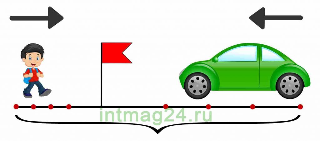
Задачи на встречное движение

В таких задачах два объекта движутся навстречу друг другу.
Задачи на встречное движение можно решать двумя способами:
1. Найти значения скорости, времени и расстояния для каждого объекта.
2. Найти скорость сближения объектов (как сумму их скоростей), общие время и расстояние. Скорость сближения — это расстояние, пройденное двумя объектами навстречу друг другу за единицу времени.

Задача 4. 

Из двух пунктов навстречу друг другу одновременно выехали два поезда и встретились через 3 часа. Первый поезд ехал со скоростью 80 км/ч, а второй – со скоростью 70 км/ч. На каком расстоянии друг от друга находятся пункты?
Решение: 
Первый способ. Найти расстояние, которое проехал каждый автобус, и сложить полученные данные:
80*3=240 (км) – проехал 1й автобус, 70*3=210 (км) – проехал 2й поезд,
240+210=450 (км) – проехали два поезда.
Второй способ. Найти скорость сближения поездов, то есть на сколько сокращалось расстояние между ними каждый час; а затем найти расстояние:
80+70=150 (км/ч), 150*3=450 (км).
Ответ: города находятся на расстоянии 450 км.

Задача 5. 

Из двух городов навстречу друг другу одновременно выехали два автобуса. Первый автобус ехал со скоростью 80 км/ч, а второй – со скоростью 70 км/ч. Какое расстояние будет между ними через 2 часа, если расстояние между городами 450 км?
Решение: 
Первый способ. Определить, сколько километров проехал каждый автобус и найти расстояние, которое осталось проехать:
80*2=160 (км)-проехал 1й автобус, 70*2=140 (км)-проехал 2й автобус,
160+140=300 (км)-проехали два автобуса, 450-300=150 (км)-осталось проехать.
Второй способ. Найти скорость сближения автобусов и умножить ее на время в пути.
80*70=150 (км/ч) – скорость сближения; 150*2=300 (км) – проехали два автобуса; 450-300=150 (км) – осталось проехать.
Ответ: Через 2часа расстояние между автобусами будет 150 км.

Задачи на движение в противоположных направлениях

В таких задачах два объекта движутся в противоположных направлениях, отдаляясь друг от друга. В таком типе задачи используется скорость удаления. Задачи на движение в противоположных направлениях также можно решить двумя способами:
1. Найти значения скорости, времени и расстояния для каждого объекта.
2. Найти скорость удаления объектов (как сумму их скоростей), общие время и расстояние. Скорость удаления — это расстояние, которое увеличивается за единицу времени между двумя объектами, двигающимися в противоположных направлениях.

Задача 6. 

Два автомобиля выехали одновременно из одного и того же пункта в противоположных направлениях. Скорость первого автомобиля 100 км/ч, скорость второго – 70 км/ч. Какое расстояние будет между автомобилями через 4 часа?
Решение: 
Первый способ. Определить расстояние, которое проехал каждый автомобиль и найти сумму полученных результатов:
1) 100 · 4 = 400 (км) – проехал первый автомобиль
2) 70 · 4 = 280 (км) – проехал второй автомобиль
400 + 280 = 680 (км)
Второй способ. Найти скорость удаления, то есть значение увеличения расстояния между автомобилями за каждый час, а затем скорость удаления умножить на время в пути.
100 + 70= 170 км/ч – это скорость удаления автомобилей.
170 · 4 = 680 (км)
Ответ: Через 4 часа между автомобилями будет 680 км.

Задача 7. 

Из двух населённых пунктов, расстояние между которыми 40 км, вышли в противоположных направлениях два туриста. Первый турист шёл со скоростью 4 км/ч, а второй — 5 км/ч. Какое расстояние между туристами будет через 5 часов?
Решение: 
Первый способ. Определить сколько километров прошёл каждый из туристов за 5 часов, сложить полученные результаты, а затем к полученному расстоянию прибавить расстояние между населенными пунктами.
1) 4 · 5 = 20 (км) – прошёл первый турист;
2) 5 · 5 = 25 (км) – прошёл второй турист;
3) 20 + 25 = 45 (км);
4) 45 + 40 = 85 (км).
Второй способ. Найти скорость удаления пешеходов, затем найти пройденное расстояние, к полученному результату прибавить расстоянием между населёнными пунктами.
4 + 5 = 9 (км/ч);
9 · 5 = 45 (км);
45 + 40 = 85 (км);
Ответ: Через 5 часов расстояние между пешеходами будет 85 км.

Задачи на движение в одном направлении

В таких задачах два объекта движутся в одном направлении с разной скоростью, при этом они сближаются друг с другом или отдаляются друг от друга. Соответственно находится скорость сближения или скорость удаления объектов.

Формула нахождения скорости сближения или удаления двух объектов, которые движутся в одном направлении: из большей скорости вычесть меньшую.

Задача 8. 

Из города выехал автомобиль со скоростью 40 км/ч. Через 4 часа вслед за ним выехал второй автомобиль со скоростью 60 км/ч. Через сколько часов второй автомобиль догонит первый?,
Решение: 
Задачу можно решить с помощью уравнения.
В этом случае скорость первого автомобиля 40 км/час, время в пути на 4 часа больше, чем время второго автомобиля (или t+4). Скорость второго автомобиля 60 км/час, время в пути – t. Расстояние оба автомобиля проехали одинаковое. Поэтому можно составить уравнение: 40*(t+4)=60*t. Отсюда получаем t=8 (часов) – время в пути второго автомобиля, за которое он догонит первый.
Решение задачи без использования уравнения.
Так как на момент выезда второго автомобиля из города первый уже был в пути 4 часа, то за это время он успел удалиться от города на: 40 · 4 = 160 (км).
Второй автомобиль движется быстрее первого, значит, каждый час расстояние между автомобилями будет сокращаться на разность их скоростей: 60 — 40 = 20 (км/ч) – это скорость сближения.
Разделив расстояние между автомобилями на скорость их сближения, можно узнать, через сколько часов они встретятся: 160 : 20 = 8 (ч)
Ответ: Второй автомобиль догонит первый через 8 часов.

Задача 9. 

Из двух посёлков между которыми 5 км, одновременно в одном направлении вышли два пешехода. Скорость пешехода, идущего впереди, 4 км/ч, а скорость пешехода, идущего позади 5 км/ч. Через сколько часов после выхода второй пешеход догонит первого?
Решение: Так как второй пешеход движется быстрее первого, то каждый час расстояние между ними будет сокращаться. Значит можно определить скорость сближения пешеходов: 5 — 4 = 1 (км/ч).
Оба пешехода вышли одновременно, значит расстояние между ними равно расстоянию между посёлками (5 км). Разделив расстояние между пешеходами на скорость их сближения, узнаем через сколько второй пешеход догонит первого: 5 : 1 = 5 (ч)
Ответ: Через 5 часов второй пешеход догонит первого.

Задача 10. 

Два автомобиля выехали одновременно из одного и того же пункта в одном направлении. Скорость первого автомобиля 80 км/ч, а скорость второго – 40 км/ч.
1) Чему равна скорость удаления между автомобилями?
2) Какое расстояние будет между автомобилями через 3 часа?
3) Через сколько часов расстояние между ними будет 200 км?
Решение: 
1) 80 — 40 = 40 (км/ч) — скорость удаления автомобилей друг от друга.
2) 40 · 3 = 120 (км) – расстояние между ними через 3 часа./
3) 200 : 40 = 5 (ч) – время, через которое расстояние между автомобилями станет 200 км.
Ответ:
1) Скорость удаления между автомобилями равна 40 км/ч.
2) Через 3 часа между автомобилями будет 120 км.
3) Через 5 часов между автомобилями будет расстояние в 200 км.

Задачи на движение по реке

Рассмотрим задачи, в которых речь идёт о движении объекта по реке. Скорость любого объекта в стоячей воде называют собственной скоростью этого объекта.

Чтобы узнать скорость объекта, который движется по течению реки, надо к собственной скорости объекта прибавить скорость течения реки. Чтобы узнать скорость объекта, который движется против течения реки, надо из собственной скорости объекта вычесть скорость течения реки.

Задача 11. 

Лодка движется по реке. За сколько часов она преодолеет расстояние 120 км, если ее собственная скорость 27 км/ч, а скорость течения реки 3 км/ч?
Решение: 
1) лодка движется по течению реки.
27 + 3 = 30 (км/ч) – скорость лодки по течению реки.
120 : 30 = 4 (ч) – проплывет путь.
2) лодка движется против течения реки.
27 — 3 = 24 (км/ч) — скорость лодки против течения реки
120 : 24 = 5 (ч) – проплывет путь.
Ответ:
1) При движении по течению реки лодка потратит 4 часа на путь.
2) При движении против течения реки лодка потратит 5 часов на путь.

Итак, для решения задач на движение:

1. Основная формула:S=ν*t;
2. Нужно сделать чертеж, который поможет определить тип задачи.
3. Все цифры нужно привести в единые единицы измерения: длина и время

Заключение.

Решая много задач по данной теме, ученик обязательно научится быстро ориентироваться в понятиях «скорость», «время» и «расстояние» и быстро решать задачи всех типов.

Весь курс начальной школы (за 1-4 классы) в краткой форме на сайте edu.intmag24.ru. С помощью курса можно быстро повторить основные моменты и правила по предметам: русский язык, математика, окружающий мир.

Для решения более сложных задач на движение посмотрите, как составлять схемы и таблицы данных для наглядного представления и структурирования данных.