Точка округления (круговая точка, омбилическая точка или омбилика; название «омбилика» происходит от лат. «umbilicus» ― «пуп») ― точка на гладкой регулярной поверхности в евклидовом пространстве, в которой нормальные кривизны по всем направлениям равны.
Свойства

![]()
Омбилические точки и сеть линий кривизны поверхности. В случае общего положения существуют три топологические различные типа особенности, называемые лимон, звезда и монстар.[1]
В точке округления:
Примеры
В евклидовом пространстве с метрикой  :
:
- Сфера целиком состоит из эллиптических точек округления.
- Трёхосный эллипсоид с попарно различными осями имеет ровно 4 точки округления, все они являются эллиптическими.
- Плоскость целиком состоит из плоских омбилик.
- Обезьянье седло имеет изолированную точку округления с нулевой гауссовой кривизной в начале координат.
Обобщение
Пусть  ― гладкое многообразие произвольной размерности
  в евклидовом пространстве большей размерности. Тогда в каждой точке
  определены
  собственных значений
  пары первой и второй квадратичных форм, заданных на касательном расслоении
  . Точка называется омбиликой, если в ней набор содержит хотя бы два совпадающих числа. Множество омбилик точек имеет коразмерность 2, т.е. задается на двумя независимыми уравнениями.[2] Так, омбилические точки на поверхности общего положения изолированы (
 ), а на трёхмерном многообразии общего положения они образуют кривую (
 ).
).
Литература
- Рашевский П.К. Курс дифференциальной геометрии, — Любое издание.
- Фиников С.П. Курс дифференциальной геометрии, — Любое издание.
- Фиников С.П. Теория поверхностей, — Любое издание.
- Porteous I.R. Geometric Differentiation for the intelligence of curves and surfaces — Cambridge University Press, Cambridge, 1994.
- Struik D. J. Lectures on Classical Differential Geometry, — Addison Wesley Publ. Co., 1950. Reprinted by Dover Publ., Inc., 1988.
Примечания
- ↑ Ремизов А.О. Многомерная конструкция Пуанкаре и особенности поднятых полей для неявных дифференциальных уравнений, ― СМФН, 19 (2006), 131–170.
- ↑ Арнольд В.И. Математические методы классической механики, ― Любое издание. (Добавление 10. Кратности собственных частот и эллипсоиды, зависящие от параметров).
Физика > Ошибка округления
Ошибка округления – разница между вычисленным приближенным значением и точным математическим: округление чисел, правила округления, разница и точность.
Задача обучения
- Объяснить возможность ошибок округления при расчетах и принципы их уменьшения.
Основные пункты
- Когда производят последовательные вычисления, то ошибки округления могут накапливаться, пока не приведут к весомой погрешности.
- Увеличение количества цифр уменьшает величину возможных ошибок округления. Но это не всегда приемлемо в вычислениях вручную.
- Степень – округление чисел относительно цели расчетов и фактического значения.
Термин
- Округление – неточное решение или результат, выступающий приемлемым для определенной цели.
Ошибка округления
Ошибка округления – разница между рассчитанным приближенным числом и точным математическим показателем. Численный анализ старается оценить эту погрешность при использовании округлений в уравнениях и алгоритмах. Проблема в том, что если применяются последовательные вычисления, то первоначальная ошибка в округлении способна вырасти до весомой погрешности, которая сильно повлияет на результат.
Подсчеты редко приводят к целым числам. Поэтому мы получаем десятичное с бесконечными цифрами. Чем больше чисел используют, тем точнее подсчеты. Но в некоторых случаях это неприемлемо, особенно при расчетах вручную. Тем более, что человеческое внимание не способно уследить за такими погрешностями. Чтобы упростить процесс, числа округляют до нескольких десятых.
Например, уравнение для нахождения окружности A=πr2 довольно сложно вычислить, так как число π тянется до бесконечности (абсолютная ошибка округления числа пи), но чаще представляется как 3.14. Технически это снижает точность вычисления, но данное число достаточно близко к реальной оценке.
Однако при следующих расчетах данные будут снова округляться, а значит накапливаются ошибки. Если их много, то не миновать серьезных сдвигов в расчетах.
Вот один из таких примеров:

Округление данных чисел повлияет на ответ. Чем больше округлений, тем больше ошибок.
Ошибки округления
Даже
если предположить, что исходная информация
не содержит никаких ошибок и все
вычислительные процессы конечны и не
приводят к ошибкам ограничения, то все
равно в этом случае присутствует третий
тип ошибок – ошибки округления.
Предположим, что вычисления производятся
на машине, в которой каждое число
представляется 5-ю значащими цифрами,
и что необходимо сложить два числа
9.2654 и 7.1625, причем эти два числа являются
точными. Сумма их равна 16.4279, она содержит
6 значащих цифр и не помещается в разрядной
сетке нашей гипотетической машины.
Поэтому 6-значный результат будет
округлен
до 16.428, и при этом возникает ошибка
округления.
Так как компьютеры всегда работают с
конечным числом значащих цифр, то
потребность в округлении возникает
довольно часто.
Вопросы
округления относятся только к
действительным числам. При выполнении
операций с целыми числами потребность
в округлении не возникает. Сумма, разность
и произведение целых чисел сами являются
целыми числами; если результат слишком
велик, то это свидетельствует об ошибке
в программе. Частное от деления двух
целых чисел не всегда является целым
числом, но при делении целых чисел
дробная часть отбрасывается.
Абсолютная и относительная погрешности
Допустим,
что точная ширина стола – А=384 мм, а мы,
измерив ее, получили а=381 мм. Модуль
разности между точным значением
измеряемой величины и ее приближенным
значением называется абсолютной
погрешностью
![]() .
.
В данном примере абсолютная погрешность
3 мм. Но на практике мы никогда не знаем
точного значения измеряемой величины,
поэтому не можем точно знать абсолютную
погрешность.
Но
обычно мы знаем точность измерительных
приборов, опыт наблюдателя, производящего
измерения и т.д. Это дает возможность
составить представление об абсолютной
погрешности измерения. Если, например,
мы рулеткой измеряем длину комнаты, то
нам нетрудно учесть метры и сантиметры,
но вряд ли мы сможем учесть миллиметры.
Да в этом и нет надобности. Поэтому мы
сознательно допускаем ошибку в пределах
1 см. абсолютная погрешность длины
комнаты меньше 1 см. Измеряя длину
какого-либо отрезка миллиметровой
линейкой, мы имеем право утверждать,
что погрешность измерения не превышает
1 мм.
Абсолютная
погрешность а
приближенного числа а дает возможность
установить границы, в которых лежит
точное число А:
![]()
Абсолютная
погрешность не является достаточным
показателем качества измерения и не
характеризует точность вычислений или
измерений. Если известно, что, измерив
некоторую длину, мы получили абсолютную
погрешность в 1 см, то никаких заключений
о том, хорошо или плохо мы измеряли,
сделать нельзя. Если мы измеряли длину
карандаша в 15 см и ошиблись на 1 см, наше
измерение никуда не годится. Если же мы
измеряли 20-метровый коридор и ошиблись
всего на 1 см, то наше измерение – образец
точности. Важна
не только сама абсолютная погрешность,
но и та доля, которую она составляет от
измеренной величины.
В первом примере абс. погрешность 1 см
составляет 1/15 долю измеряемой величины
или 7%, во втором – 1/2000 или 0.05%. Второе
измерение значительно лучше.
Относительной
погрешностью называют отношение
абсолютной погрешности к абсолютному
значению приближенной величины:
![]() .
.
В
отличие от абсолютной погрешности,
которая обычно есть величина размерная,
относительная погрешность всегда есть
величина безразмерная. Обычно ее выражают
в %.
Пример
При измерении
длины в 5 см допущена абсолютная
погрешность в 0.1 см. Какова относительная
погрешность? (Ответ 2%)
При
подсчете числа жителей города, которое
оказалось равным 2
000
000,
допущена
погрешность 100 человек. Какова относительная
погрешность? (Ответ
0.005%)
Результат
всякого измерения выражается числом,
лишь приблизительно характеризующим
измеряемую величину. Поэтому при
вычислениях мы имеем дело с приближенными
числами. При записи приближенных чисел
принимается, что последняя цифра справа
характеризует величину абсолютной
погрешности.
Например,
если записано 12.45, то это не значит, что
величина, характеризуемая этим числом,
не содержит тысячных долей. Можно
утверждать, что тысячные доли при
измерении не учитывались, следовательно,
абсолютная погрешность меньше половины
единицы последнего разряда:
![]() .
.
Аналогично, относительно приближенного
числа 1.283, можно сказать, что абсолютная
погрешность меньше 0.0005:![]() .
.
Приближенные
числа принято записывать так, чтобы
абсолютная погрешность не превышала
единицы последнего десятичного разряда.
Или, иначе говоря, абсолютная
погрешность приближенного числа
характеризуется числом десятичных
знаков после запятой.
Как же
быть, если при тщательном измерении
какой-нибудь величины получится, что
она содержит целую единицу, 2 десятых,
5 сотых, не содержит тысячных, а
десятитысячные не поддаются учету? Если
записать 1.25, то в этой записи тысячные
не учтены, тогда как на самом деле мы
уверены, что их нет. В таком случае
принято ставить на их месте 0, – надо
писать 1.250. Таким образом, числа 1.25 и
1.250 обозначают не одно и то же. Первое –
содержит тысячные; мы только не знаем,
сколько именно. Второе – тысячных не
содержит, о десятитысячных ничего
сказать нельзя.
Сложнее
приходится при записи больших приближенных
чисел. Пусть число жителей деревни равно
2000 человек, а в городе приблизительно
457
000
жителей. Причем относительно города в
тысячах мы уверены, но допускаем
погрешность в сотнях и десятках. В первом
случае нули в конце числа указывают на
отсутствие сотен, десятков и единиц,
такие нули мы назовем значащими;
во втором случае нули указывают на наше
незнание числа сотен, десятков и единиц.
Такие нули мы назовем незначащими.
При записи приближенного числа,
содержащего нули надо дополнительно
оговаривать их значимость. Обычно нули
– незначащие. Иногда на незначимость
нулей можно указывать, записывая число
в экспоненциальном виде (457*103).
Сравним
точность двух приближенных чисел 1362.3
и 2.37. В первом абсолютная погрешность
не превосходит 0.1, во втором – 0.01. Поэтому
второе число выглядит более точным, чем
первое.
Подсчитаем
относительную погрешность. Для первого
числа
![]() ;
;
для второго![]() .
.
Второе число значительно (почти в 100
раз) менее точно, чем первое. Получается
это потому, что в первом числе дано 5
верных (значащих) цифр, тогда как во
втором – только 3.
Все
цифры приближенного числа, в которых
мы уверены, будем называть верными
(значащими) цифрами. Нули сразу справа
после запятой не бывают значащими, они
лишь указывают на порядок стоящих правее
значащих цифр. Нули в крайних правых
позициях числа могут быть как значащими,
так и не значащими. Например, каждое из
следующих чисел имеет 3 значащие цифры:
283*105,
200*102,
22.5, 0.0811, 2.10, 0.0000458.
Пример
Сколько
значащих (верных) цифр в следующих
числах:
0.75
(2), 12.050 (5), 1875*105
(4), 0.06*109
(1)
Оценить
относительную погрешность следующих
приближенных чисел:
0.989
(0.1%),
нули
значащие: 21000 (0.005%),
0.000
024
(4%),
0.05 (20%)
Нетрудно
заметить, что для примерной оценки
относительной погрешности числа
достаточно подсчитать количество
значащих цифр. Для числа, имеющего только
одну значащую цифру относительная
погрешность около 10%;
с
2-мя значащими цифрами – 1%;
с
3-мя значащими цифрами – 0.1%;
с
4-мя значащими цифрами – 0.01% и т.д.
При
вычислениях с приближенными числами
нас будет интересовать вопрос: как,
исходя из данных приближенных чисел,
получить ответ с нужной относительной
погрешностью.
Часто
при этом все исходные данные приходится
брать с одной и той же погрешностью,
именно с погрешностью наименее точного
из данных чисел. Поэтому часто приходится
более точное число заменять менее точным
– округлять.
округление
до десятых 27.136
27.1,
округление
до целых 32.8
33.
Правило
округления: Если крайняя левая из
отбрасываемых при округлении цифр
меньше 5, то последнюю сохраняемую цифру
не изменяют; если крайняя левая из
отбрасываемых цифр больше 5 или если
она равна 5, то последнюю сохраняемую
цифру увеличивают на 1.
Пример
округлить
до десятых 17.96 (18.0)
округлить
до сотых 14.127 (14.13)
округлить,
сохранив 3 верные цифры: 83.501 (83.5), 728.21
(728), 0.0168835 (0.01688).
Соседние файлы в предмете [НЕСОРТИРОВАННОЕ]
- #
- #
- #
- #
- #
- #
- #
- #
- #
- #
- #
Компенсация погрешностей при операциях с числами с плавающей запятой
Работа посвящена погрешностям округления, возникающим при вычислениях у чисел с плавающей запятой. Здесь будут кратко рассмотрены следующие темы: «Представление вещественных чисел», «Способы нахождения погрешностей округления у чисел с плавающей запятой» и будет приведен пример компенсации погрешностей округления.
В данной работе примеры приведены на языке програмиирования C.
Представление вещественных чисел
Рассмотрим представление конечного действительного числа в стандарте IEEE 754-2008 в виде выражения, которое характеризуется тремя элеменами: S (0 или 1), мантисса M и порядок E:
v = -1S * b(E — BIAS) * M
- основанием b (стандартом определено три двоичных формата и два десятичных);
- длиной мантиссы p, определяющей точность представления числа, измеряется в цифрах (двоичных или десятичных);
- максимальным значением порядка emax;
- минимальным значением порядка emin; стандарт требует, чтобы выполнялось условие:
emin = 1-emax - BIAS (смещение); порядок записывается в т. н. смещенной форме, т. е.
реальное значение показателя степени равно E-BIAS.
Ниже в таблице даны параметры стандартных форматов чисел с плавающей запятой. Здесь: w — ширина битового поля для представления порядка, t — ширина битового поля для представления мантиссы, k — полная ширина битовой строки.
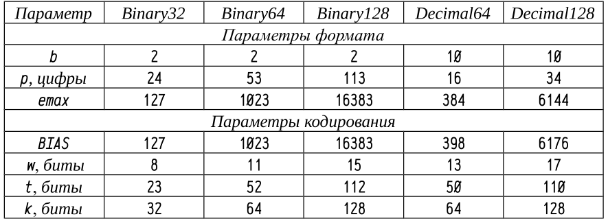
В следующией таблице представлены диапазоны изменения и точность стандартных 32 и 64-х разрядных форматов вещественных чисел с плавающей запятой.

Здесь «Точноть, Эпсилон» — наименьшее число, для которого истинно выражение:
1 + EPSILON != 1Данная величина «Эпсилон», характеризует относительную точность операций сложения и вычитания: если прибавляемая к x или вычитаемая из x величина меньше, чем epsilon*x, то результат останется равен x. На практике, в ряде случаев, при использовании в аддитивных операциях величин, приближающихся по порядку к epsilon*x, начинают сказываться погрешности округления меньшего слагаемого. О таких ситуациях и пойдет речь в данной работе.
Рассмотрим представление вещественного числа для типа данных float(Binary32).

В данном примере:
- Число V = 0,1562510
- Знак S = 0, т.е. +
- Порядок (E — BIAS) = 011111002 — 011111112 = 12410 — 12710 = -310
- Мантисса M = 1,010000000000000000000002
Таким образом, число V = 1,012*210-310 = 1012*210-510 = 510*210-510 = 0,1562510
Заметим, что при выполнении операций с вещественными числами часто результат не будет помещаться в N-разрядные матиссы, т.е. будет происходить округление. Округление в одной вычислительной операции не превывает порядок EPSILON/2, но когда нам требуется делать много операций, то для повышения точности вычисления результата нам надо научиться находить, насколько именно результат каждой конкретной операции округлён.
Более подробно про округления и нарушение аксиоматики рассказано в файле makarov_float.pdf (ссылка на материал внизу).
Способы нахождения погрешностей округления у чисел с плавающей запятой
Данную проблему исследовали многие специалисты, наиболее известными из них являются: Дэвид Голдберг, Уильям Кэхен, Джонатан Ричард Шевчук.
Ниже мы рассмотрим алгоримы нахождения погрешностей округления, приведенные в работе Шевчука, на примере двух функций:
- TwoSum — функция нахождения погрешности округления при сложении.
- TwoProduct — функция нахождения погрешности округления при умножении.
Для правильного понимания указанных алгоритмов мы будем опираться на теоремы, которые рассмотрены в работе Шевчука. Теоремы приводим без доказательств.
Говоря, что число a является p-битовым числом, имеется ввиду, что длина матиссы числа a представляется p битами.
TwoSum
Теорема: пусть числа a и b являются p-битовыми числами с плавающей запятой, где p >= 3, тогда следуя данному алгоритму мы получим 2 числа: x и y, для которых выполняется условие: a + b = x + y. Причем x является апроксиммацией суммы a и b, а y является погрешностью округления вычисления числа x.

TwoProduct
В действительности, алогритм находжения погрешности огругления при умножении двух вещественных чисел состоит из 2-х функций: Split — вспомогательной функции и функции TwoProduct, где мы находим погрешность.
Рассмотрим алгоритм функции Split.
Split
Теорема: число a — p-битовое число с плавающей запятой, где p >= 3. Выберем точку разрыва s, где p/2 <= s <= p-1. Следуя алгоритму, получим (p — s)-битное число — число a_hi и (s-1)-битное число — a_lo, где |a_hi| >= |a_low| и a = a_hi + a_low.

Теперь перейдем к анализу функции TwoProduct.
TwoProduct
Теорема: пусть числа a и b являются p-битовыми числами с плавающей запятой, где p >= 6. Тогда, выполняя данный алгоритм, мы получим 2 числа: x и y, для которых выполняется условие: a*b = x + y. Причем x является апроксиммацией произведения чисел a и b, а число y является погрешностью округления вычисления числа x.

Видно, что конечный результат представляется парой N-битовых вещественных чисел: результат + погрешность. Причем второе должно иметь порядок не более EPSILON по отношению к первому.
Пример компесации погрешностей округления у чисел с плавающей запятой
Теперь перейдем к практическим расчетам, которые построены на алгоритмах Шевчука. Найдем погрешности округления при сложении и умножении чисел с плавающей запятой и проанализируем, как накапливается погрешность.
Погрешность округления суммы
Приведем пример простейшей программы суммирования:
#include <stdio.h>
#include <math.h>

int main() {
    float val = 2.7892;
    printf("%0.7g n", val);
    val = val/10000000000.0;
    float result = 0.0;
    for (long long i = 0; i < 10000000000; i++) {
        result += val;
    }
    printf("%0.7g n", result);
    return 0;
}
В результате работы программы, мы должны получить два одинаковых числа: 2,7892 и 2,7892. Но в консоль было выведено: 2,7892 и 0,0078125. Отсюда видно, что погрешность накопилась очень большая.
Теперь попробуем сделать то же самое, но, используя алгоритм Шевчука, будем накапливать погрешность в отдельную переменную, а затем скомпенсируем результат путем прибавления ошибки к главной переменной суммы.
#include <stdio.h>
#include <math.h>

float TwoSum(float a, float b, float& error) {
    float x = a + b;
    float b_virt = x - a;
    float a_virt = x - b_virt;
    float b_roundoff = b - b_virt;
    float a_roudnoff = a - a_virt;
    float y = a_roudnoff + b_roundoff;
    error += y;
    return x;
}

int main() {
    float val = 2.7892;
    printf("%0.7g n", val);
    val = val/10000000000.0;
    float result = 0.0;
    float error = 0.0;
    for (long long i = 0; i < 10000000000; i++) {
        result = TwoSum(result, val, error);
    }
    result += error;
    printf("%0.7g n", result);
    return 0;
}
В итоге мы получаем 2 числа: 2,7892 и 0,015625. Результат улучшился, но погрешность все равно дает о себе знать. В данном примере не была учтена погрешость, возникающая в операции сложения, в функции TwoSum():
error += y;
Будем компенсировать результат на каждой итерации цикла и перезаписывать ошибку в переменную, которая накапливает погрешность округления в операции суммирования. Для этого модифицируем функцию TwoSum(): добавим переменную isNull типа bool которая указывает на то, стоит ли нам накапливать погрешность или же стоит ее перезаписать.
В итоге, result будет представляться 2 переменными: result — главная переменная, error1 — погрешность операции result += val.
Код будет выглядеть следующим образом:
#include <stdio.h>
#include <math.h>

float TwoSum(float a, float b, float& error, bool isNull) {
    float x = a + b;
    float b_virt = x - a;
    float a_virt = x - b_virt;
    float b_roundoff = b - b_virt;
    float a_roudnoff = a - a_virt;
    float y = a_roudnoff + b_roundoff;
    if (isNull) {
        error = y;
    } else {
        error += y;
    }
    return x;
}

int main() {
    float val = 2.7892;
    printf("%0.7g n", val);
    val = val/10000000000.0;
    float result = 0.0;
    float error1 = 0.0;
    for (long long i = 0; i < 10000000000; i++) {
        result = TwoSum(result, val, error1, false);
        result = TwoSum(error1, result, error1, true);
    }
    printf("%0.7g n", result);
    return 0;
}
Программа выведет числа: 2,7892 и 2,789195.
Заметим, что здесь не была учтена погрешность округления, возникающая в операции умножения:
val = val*(1/10000000000.0);
Учтем эту погрешность путем добавления функций учета погрешностей умножения, которые разработал Д.Р. Шевчук. При этом переменная val будет представлена двумя переменными:
val_real = val + errorMult
Таким образом, result будет представляться 3 переменными: result — главная переменная, error1 — погрешность операции result += val, error2 — погрешность операции result += errorMult.
Так же мы будем складывать переменные error1 и error2, а погрешность от этой операции записывать в error2.
В итоге, код:
#include <stdio.h>
#include <math.h>

float TwoSum(float a, float b, float& error, bool isNull) {
//isNull отвечает за то, стоит ли нам накопить возникающую погрешность
// или же стоит перепизаписать ее
    float x = a + b;
    float b_virt = x - a;
    float a_virt = x - b_virt;
    float b_roundoff = b - b_virt;
    float a_roudnoff = a - a_virt;
    float y = a_roudnoff + b_roundoff;
    if (isNull) {
        error = y;
    } else {
        error += y;
    }
    return x;
}

void Split(float a, int s, float& a_hi, float& a_lo) {
    float c = (pow(2, s) + 1)*a;
    float a_big = c - a;
    a_hi = c - a_big;
    a_lo = a - a_hi;
}

float TwoProduct(float a, float b, float& err) {
    float x = a*b;
    float a_hi, a_low, b_hi, b_low;
    Split(a, 12, a_hi, a_low);
    Split(b, 12, b_hi, b_low);
    float err1, err2, err3;
    err1 = x - (a_hi*b_hi);
    err2 = err1 - (a_low*b_hi);
    err3 = err2 - (a_hi*b_low);
    err += ((a_low * b_low) - err3);
    return x;
}

int main() {
    float val = 2.7892;
    printf("%0.7g n", val);
    float errorMult = 0;//погрешность умножения
    val = TwoProduct(val, 1.0/10000000000.0, errorMult);
    float result = 0.0;
    float error1 = 0.0;
    float error2 = 0.0;
    for (long long i = 0; i < 10000000000; i++) {
        result = TwoSum(result, val, error1, false);
        result = TwoSum(result, errorMult, error2, false);
        error1 = TwoSum(error2, error1, error2, true);
        result = TwoSum(error1, result, error1, true);
    }
    printf("%0.7g n", result);
    return 0;
}
В консоль были выведены следующие числа: 2,7892 и 2,789195.
Это говорит о том, что погрешность округления умножения достаточно мала, чтоб проявиться даже на 10 миллиардах итераций. Данный результат является максимально приближенным к исходному числу, если учитывать погрешности в операциях сложения и умножения. Для получение более точного результата можно ввести дополнительные переменные, учитывающие погрешности. Скажем, добавить переменную, учитывающую погрешность в операции накопления основной погрешности в функции TwoSum(). Тогда эта погрешность будет иметь порядок EPSILON2, по отношению к главному результату (первая погрешность будет иметь порядок EPSILON).
Погрешность округления умножения
Посчитаем число 1.0012101 в цикле, т.е. сделаем следующие:
#include <stdio.h>
#include <math.h>

int main() {
    float val = 1.0012;
    float result = 1.0012;
    for (long long i = 0; i < 100; i++) {
        result *= val;
    }
    printf("%0.15g n", result);
    return 0;
}
Заметим, что точный результат, с точностью до пятнадцатого знака после запятой, равен 1.128768638496750. Мы получим: 1.12876391410828. Как видно, погрешность оказалось достаточно большой.
Выведем переменную val, приведя ее к типу данных double, и посмотрим, что в нее на самом деле записалось:
printf("%0.15g n", (double)val);
Мы получим число 1.00119996070862. Это говорит о том, что в программировании даже самая точная константа не является ни надежной, ни константой. Поэтому, наш реальный точный результат будет равен 1.128764164435784, с точностью до пятнадцатого знака после запятой.
Теперь попробуем улучшить полученный ранее результат. Для этого введем компенсацию результата вычислений, путем учета погрешности округления в операции умножения. Так же будем пытаться прибавлять накопившуюся погрешность к переменной result на каждом шаге.
Код:
#include <stdio.h>
#include <math.h>

float TwoSum(float a, float b, float& error, bool isNull) {
//isNull отвечает за то, стоит ли нам накопить возникающую погрешность
// или же стоит перепизаписать ее
    float x = a + b;
    float b_virt = x - a;
    float a_virt = x - b_virt;
    float b_roundoff = b - b_virt;
    float a_roudnoff = a - a_virt;
    float y = a_roudnoff + b_roundoff;
    if (isNull) {
        error = y;
    } else {
        error += y;
    }
    return x;
}

void Split(float a, int s, float& a_hi, float& a_lo) {
    float c = (pow(2, s) + 1)*a;
    float a_big = c - a;
    a_hi = c - a_big;
    a_lo = a - a_hi;
}

float TwoProduct(float a, float b, float& err) {
    float x = a*b;
    float a_hi, a_low, b_hi, b_low;
    Split(a, 12, a_hi, a_low);
    Split(b, 12, b_hi, b_low);
    float err1, err2, err3;
    err1 = x - (a_hi*b_hi);
    err2 = err1 - (a_low*b_hi);
    err3 = err2 - (a_hi*b_low);
    err += ((a_low * b_low) - err3);
    return x;
}

int main() {
    float val = 1.0012;
    float result = 1.0012;
    float errorMain = 0.0;
    for (long long i = 0; i < 100; i++) {
        result = TwoProduct(result, val, errorMain);
        result = TwoSum(errorMain, result, errorMain, true);
    }
    printf("%0.15g n", result);
    return 0;
}
Программа выводит следующее число: 1.12876415252686. Мы получили погрешность 1.0e-008, что меньше чем EPSILON/2 для типа данных float. Таким образом, данный результат можно считать достаточно хорошим.
Итоги
1) В данной работе было рассмотрено представление чисел с плавающей запятой в формате стандарта IEEE 754-2008.
2) Был показан способ нахождения погрешностей округления в операциях сложения и умножения у чисел с плавающей запятой.
3) Были рассмотрены простые примеры компенсации погрешностей округления у чисел с плавающей запятой.
Работу выполнил Виктор Фадеев.
Консультировал Макаров А.В.
P.S. Спасибо за найденные ошибки пользователям:
xeioex, Albom.
Использованная литература
- Работы Макарова Андрея Владимировича на тему «Представление вещественных чисел». В файле makarov_float .pdf показано, как возникают погрешности округления у чисел с плавающей запятой.
- Википедия. Число одинарной точности.
- Adaptive Precision Floating-Point Arithmetic
and Fast Robust Geometric Predicates
Jonathan Richard Shewchuk
Ошибки округления , [1] также называется ошибка округления , [2] представляют собой разность между результатом полученного по заданному алгоритму с использованием точного арифметическим и результат получает тем же самый алгоритм с использованием конечной точности, округленная арифметики. [3] Ошибки округления возникают из-за неточности в представлении действительных чисел и выполняемых с ними арифметических операций. Это форма ошибки квантования . [4] При использовании приближенных уравнений или алгоритмов, особенно при использовании конечного числа цифр для представления действительных чисел (которые теоретически имеют бесконечное количество цифр), одна из целейчисленный анализ предназначен для оценки ошибок вычислений. [5] Ошибки вычислений, также называемые числовыми ошибками , включают как ошибки усечения, так и ошибки округления.
Когда выполняется последовательность вычислений с вводом, включающим любую ошибку округления, ошибки могут накапливаться, иногда доминируя в вычислении. В плохо обусловленных проблемах может накапливаться значительная ошибка. [6]
Короче говоря, есть два основных аспекта ошибок округления, связанных с численными расчетами: [7]
- Цифровые компьютеры имеют ограничения по величине и точности их способности представлять числа.
- Некоторые численные операции очень чувствительны к ошибкам округления. Это может быть связано как с математическими соображениями, так и с тем, как компьютеры выполняют арифметические операции.
Ошибка представления
Ошибка, возникающая при попытке представить число с помощью конечной строки цифр, является формой ошибки округления, называемой ошибкой представления . [8] Вот несколько примеров ошибок представления в десятичных представлениях:
| Обозначение |
Представление |
Приближение |
Ошибка |
|---|---|---|---|
| 1/7 | 0. 142 857 | 0,142 857 | 0,000 000 142 857 |
| пер 2 | 0,693 147 180 559 945 309 41 … | 0,693 147 | 0,000 000 180 559 945 309 41 … |
| журнал 10 2 | 0,301 029 995 663 981 195 21 … | 0,3010 | 0,000 029 995 663 981 195 21 … |
| 3 √ 2 | 1,259 921 049 894 873 164 76 … | 1,25992 | 0,000 001 049 894 873 164 76 … |
| √ 2 | 1,414 213 562 373 095 048 80 … | 1,41421 | 0,000 003 562 373 095 048 80 … |
| е | 2,718 281 828 459 045 235 36 … | 2,718 281 828 459 045 | 0,000 000 000 000 000 235 36 … |
| π | 3,141 592 653 589 793 238 46 … | 3,141 592 653 589 793 | 0,000 000 000 000 000 238 46 … |
Увеличение числа цифр, разрешенных в представлении, снижает величину возможных ошибок округления, но любое представление, ограниченное конечным числом цифр, все равно вызовет некоторую степень ошибки округления для несчетного количества действительных чисел. Дополнительные цифры, используемые на промежуточных этапах вычислений, называются защитными цифрами . [9]
Многократное округление может привести к накоплению ошибок. [10] Например, если 9,945309 округляется до двух десятичных знаков (9,95), а затем снова округляется до одного десятичного знака (10,0), общая ошибка составляет 0,054691. Округление 9,945309 до одного десятичного знака (9,9) за один шаг приводит к меньшей ошибке (0,045309). Обычно это происходит при выполнении арифметических операций (см. « Потеря значимости» ).
Система счисления с плавающей точкой
По сравнению с системой счисления с фиксированной запятой, система счисления с плавающей запятой более эффективна при представлении действительных чисел, поэтому она широко используется в современных компьютерах. Пока реальные цифры бесконечны и непрерывны, система счисления с плавающей запятой конечно и дискретно. Таким образом, ошибка представления, которая приводит к ошибке округления, возникает в системе счисления с плавающей запятой.
Обозначение системы счисления с плавающей запятой
Система счисления с плавающей запятой характеризуется целые числа:
- : основание или основание
- : точность
- : диапазон экспоненты, где это нижняя граница и это верхняя граница
- Любой имеет следующий вид:
- куда целое число такое, что для , а также целое число такое, что .
Нормализованная система с плавающей запятой
- Система счисления с плавающей запятой нормализуется, если первая цифра всегда отличен от нуля, если только число не равно нулю. [3] Поскольку мантиссамантисса ненулевого числа в нормированной системе удовлетворяет . Таким образом, нормализованная форма ненулевого числа с плавающей запятой IEEE : куда . В двоичном формате первая цифра всегдапоэтому он не записывается и называется неявным битом. Это дает дополнительный бит точности, так что ошибка округления, вызванная ошибкой представления, уменьшается.
- Поскольку система счисления с плавающей запятой является конечным и дискретным, он не может представлять все действительные числа, что означает, что бесконечные действительные числа могут быть аппроксимированы только некоторыми конечными числами с помощью правил округления . Приближение заданного действительного числа с плавающей запятой к можно обозначить.
- Общее количество нормализованных чисел с плавающей запятой равно
-
- , куда
- считает выбор знака, положительный или отрицательный
- считает выбор первой цифры
- считает оставшуюся мантиссу
- считает выбор показателей
- считает тот случай, когда число .
- , куда
Стандарт IEEE
В стандарте IEEE база двоичная, т.е., и используется нормализация. Стандарт IEEE хранит знак, показатель степени и мантиссу в отдельных полях слова с плавающей запятой, каждое из которых имеет фиксированную ширину (количество бит). Два наиболее часто используемых уровня точности для чисел с плавающей запятой — это одинарная точность и двойная точность.
| Точность |
Знак (биты) |
Экспонента (биты) |
Мантисса (биты) |
|---|---|---|---|
| Одинокий | 1 | 8 | 23 |
| Двойной | 1 | 11 | 52 |
Машинный эпсилон
Машинный эпсилон может использоваться для измерения уровня ошибки округления в системе счисления с плавающей запятой. Вот два разных определения. [3]
- Машинный эпсилон, обозначаемый , — максимально возможная абсолютная относительная ошибка представления ненулевого действительного числа в системе счисления с плавающей запятой.
- Машинный эпсилон, обозначаемый , это наименьшее число такой, что . Таким образом, в любое время .
Ошибка округления при разных правилах округления
Существует два распространенных правила округления: округление за отрезком и округление до ближайшего. Стандарт IEEE использует округление до ближайшего.
- По очереди : Основание- расширение усекается после цифра.
- Это правило округления смещено, потому что оно всегда приближает результат к нулю.
- Округление до ближайшего : устанавливается равным ближайшему числу с плавающей запятой к . При равенстве используется число с плавающей запятой, последняя сохраненная цифра которого четная.
- Для стандарта IEEE, где базовый является , это означает, что когда есть ничья, она округляется так, чтобы последняя цифра была равна .
- Это правило округления более точное, но более затратное с точки зрения вычислений.
- Округление таким образом, чтобы последняя сохраненная цифра была даже при равенстве, гарантирует, что она не округляется систематически в большую или меньшую сторону. Это сделано для того, чтобы избежать возможности нежелательного медленного отклонения в длинных вычислениях просто из-за смещения округления.
- В следующем примере показан уровень ошибки округления в соответствии с двумя правилами округления. [3] Правило округления, округление до ближайшего, в целом приводит к меньшей ошибке округления.
| Икс |
По очереди |
Ошибка округления |
Округление до ближайшего |
Ошибка округления |
|---|---|---|---|---|
| 1,649 | 1.6 | 0,049 | 1.6 | 0,049 |
| 1,650 | 1.6 | 0,050 | 1,7 | 0,050 |
| 1,651 | 1.6 | 0,051 | 1,7 | -0,049 |
| 1,699 | 1.6 | 0,099 | 1,7 | -0,001 |
| 1,749 | 1,7 | 0,049 | 1,7 | 0,049 |
| 1,750 | 1,7 | 0,050 | 1,8 | -0,050 |
Расчет ошибки округления в стандарте IEEE
Предположим, что используется округление до ближайшего и двойная точность IEEE.
- Пример: десятичное число может быть преобразован в
Поскольку бит справа от двоичной точки — это и за ним следуют другие ненулевые биты, правило округления до ближайшего требует округления, то есть добавления немного к немного. Таким образом, нормализованное представление с плавающей запятой в стандарте IEEE является
- .
- Теперь ошибку округления можно вычислить при представлении с участием .
Это представление получается путем отбрасывания бесконечного хвоста
из правого хвоста, а затем добавил на этапе округления.
- потом .
- Таким образом, ошибка округления равна .
Измерение ошибки округления с помощью машинного эпсилона
Машина эпсилон может использоваться для измерения уровня ошибки округления при использовании двух вышеупомянутых правил округления. Ниже приведены формулы и соответствующие доказательства. [3] Здесь используется первое определение машинного эпсилон.
Теорема
- По очереди:
- Округление до ближайшего:
Доказательство
Позволять куда , и разреши быть представлением с плавающей запятой . Поскольку используется последовательное нарезание,
* Чтобы определить максимум этой величины, необходимо найти максимум числителя и минимум знаменателя. С (нормализованная система), минимальное значение знаменателя равно . Числитель ограничен сверху. Таким образом,. Следовательно,для порезки. Доказательство для округления до ближайшего аналогично.
- Обратите внимание, что первое определение машинного эпсилон не совсем эквивалентно второму определению при использовании правила округления до ближайшего, но оно эквивалентно для последовательного перехода.
Ошибка округления, вызванная арифметикой с плавающей запятой
Даже если некоторые числа могут быть представлены точно числами с плавающей запятой и такие числа называются машинными числами , выполнение арифметических операций с плавающей запятой может привести к ошибке округления в окончательном результате.
Дополнение
Машинное сложение состоит из выравнивания десятичных знаков двух добавляемых чисел, их сложения и последующего сохранения результата как числа с плавающей запятой. Само сложение может быть выполнено с более высокой точностью, но результат должен быть округлен до указанной точности, что может привести к ошибке округления. [3]
Например, добавив к в IEEE двойной точности следующим образом:
- Это сохранено как поскольку в стандарте IEEE используется округление до ближайшего. Следовательно, равно в IEEE двойной точности и ошибка округления .
Из этого примера видно, что при сложении большого числа и малого числа может возникнуть ошибка округления, поскольку сдвиг десятичных знаков в мантиссах для согласования показателей степени может вызвать потерю некоторых цифр.
Умножение
В общем, продукт -цифровые мантиссы содержат до цифр, поэтому результат может не соответствовать мантиссе. [3] Таким образом, в результат будет включена ошибка округления.
- Например, рассмотрим нормализованную систему счисления с плавающей запятой с основанием и цифры мантиссы не более . потом а также . Обратите внимание, что но так как там самое большее цифры мантиссы. Ошибка округления будет.
Подразделение
В общем, частное -цифровые мантиссы могут содержать более -цифры. [3] Таким образом, в результат будет включена ошибка округления.
- Например, если приведенная выше нормализованная система счисления с плавающей запятой все еще используется, то но . Итак, хвост отрезан.
Вычитающая отмена
Вычитание двух почти равных чисел называется вычитанием . [3]
- Когда начальные цифры отменяются, результат может быть слишком маленьким для точного представления, и он будет представлен просто как .
- Например, пусть и здесь используется второе определение машинного эпсилон. Какое решение?
Известно, что а также почти равные числа, и . Однако в системе счисления с плавающей запятой. Несмотря на то что достаточно большой, чтобы быть представленным, оба экземпляра были округлены, давая .
- Например, пусть и здесь используется второе определение машинного эпсилон. Какое решение?
- Даже с несколько большим , в типичных случаях результат по-прежнему существенно ненадежен. Нет особой веры в точность значения, потому что наибольшая неопределенность в любом числе с плавающей запятой — это цифры в крайнем правом углу.
- Например, . Результат ясно представима, но в это мало веры.
Накопление ошибки округления
Ошибки могут увеличиваться или накапливаться, когда последовательность вычислений применяется к начальному входу с ошибкой округления из-за неточного представления.
Нестабильные алгоритмы
Алгоритм или численный процесс называется стабильным, если небольшие изменения на входе вызывают только небольшие изменения на выходе, и называется нестабильным, если производятся большие изменения на выходе. [11]
Последовательность вычислений обычно происходит при запуске какого-либо алгоритма. Количество ошибок в результате зависит от стабильности алгоритма . Ошибка округления будет увеличиваться нестабильными алгоритмами.
Например, для с участием данный. Легко показать, что. Предполагать это наше начальное значение и имеет небольшую ошибку представления , что означает, что начальный вход в этот алгоритм вместо того . Затем алгоритм выполняет следующую последовательность вычислений.
Ошибка округления увеличивается в последующих вычислениях, поэтому этот алгоритм нестабилен.
Плохо обусловленные проблемы
Даже если используется стабильный алгоритм, решение проблемы может быть неточным из-за накопления ошибок округления, когда сама проблема плохо обусловлена .
Число обусловленности проблемы — это отношение относительного изменения решения к относительному изменению входных данных. [3] Проблема хорошо обусловлена, если небольшие относительные изменения входных данных приводят к небольшим относительным изменениям в решении. В противном случае проблема плохо обусловлена . [3] Другими словами, проблема является плохо обусловленной, если ее число условий «намного больше», чем.
Число обусловленности вводится как мера ошибок округления, которые могут возникнуть при решении плохо обусловленных задач. [7]
Пример из реального мира: отказ ракеты «Патриот» из-за увеличения ошибки округления

Американская ракета Пэтриот
25 февраля 1991 года, во время войны в Персидском заливе, американская ракетная батарея «Пэтриот» в Дхаране, Саудовская Аравия, не смогла перехватить приближающуюся иракскую ракету «Скад». Скад врезался в казармы американской армии и убил 28 солдат. Отчет тогдашней Главной бухгалтерииозаглавленный «Противоракетная оборона Patriot: проблема программного обеспечения, приведшая к отказу системы в Дахране, Саудовская Аравия», сообщает о причине сбоя: неточный расчет времени с момента загрузки из-за компьютерных арифметических ошибок. В частности, время в десятых долях секунды, измеренное внутренними часами системы, было умножено на 10, чтобы получить время в секундах. Этот расчет был выполнен с использованием 24-битного регистра с фиксированной запятой. В частности, значение 1/10, которое имеет неограниченное двоичное расширение, было прервано на 24 бита после точки счисления. Небольшая ошибка прерывания, умноженная на большое число, дающее время в десятых долях секунды, привела к значительной ошибке. Действительно, батарея Patriot проработала около 100 часов,и простой расчет показывает, что результирующая временная ошибка из-за увеличенной ошибки прерывания составила около 0,34 секунды. (Число 1/10 равно. Другими словами, двоичное разложение 1/10 равно. Теперь 24-битный регистр в Патриоте хранится вместо вводя ошибку двоичный, или около десятичный. Умножая на количество десятых долей секунды в часов дает ). Скад едет примерно1676 метров в секунду, то есть за это время проходит более полукилометра. Этого было достаточно, чтобы приближающийся Скад находился за пределами «ворот дальности», которые отслеживал Патриот. По иронии судьбы, тот факт, что вычисление плохого времени было улучшено в некоторых частях кода, но не во всех, способствовал возникновению проблемы, поскольку это означало, что неточности не отменялись. [12]
См. Также
- Точность (арифметика)
- Усечение
- Округление
- Потеря значимости
- Плавающая запятая
- Алгоритм суммирования Кахана
- Машина эпсилон
- Полином Уилкинсона
Ссылки
- ↑ Butt, Rizwan (2009), Введение в численный анализ с использованием MATLAB , Jones & Bartlett Learning, стр. 11–18, ISBN 978-0-76377376-2
- ^ Ueberhuber, Christoph W. (1997), Численный 1: Методы, программное обеспечение и анализ ., М., С. 139-146, ISBN 978-3-54062058-7
- ^ Б с д е е г ч я J K Форрестер, Дик (2018). Math / Comp241 Численные методы (конспекты лекций) . Колледж Дикинсона .
- ^ Аксой, Пелин; ДеНардис, Лаура (2007), Информационные технологии в теории , Cengage Learning, стр. 134, ISBN 978-1-42390140-2
- ^ Ральстон, Энтони; Рабиновиц, Филип (2012), Первый курс численного анализа , Dover Books on Mathematics (2-е изд.), Courier Dover Publications, стр. 2–4, ISBN 978-0-48614029-2
- ^ Чапман, Стивен (2012), Программирование MATLAB с приложениями для инженеров , Cengage Learning, стр. 454, ISBN 978-1-28540279-6
- ^ a b Чапра, Стивен (2012). Прикладные численные методы с MATLAB для инженеров и ученых (3-е изд.). ISBN компании McGraw-Hill Companies, Inc. 9780073401102.
- ^ Laplante, Филип А. (2000). Словарь компьютерных наук, инженерии и технологий . CRC Press . п. 420. ISBN 978-0-84932691-2.
- ^ Хайэм, Николас Джон (2002). Точность и устойчивость численных алгоритмов (2-е изд.). Общество промышленной и прикладной математики (SIAM). С. 43–44. ISBN 978-0-89871521-7.
- Перейти ↑ Volkov, EA (1990). Численные методы . Тейлор и Фрэнсис . п. 24. ISBN 978-1-56032011-1.
- ^ Коллинз, Чарльз (2005). «Состояние и стабильность» (PDF) . Департамент математики Университета Теннесси . Проверено 28 октября 2018 .
- ^ Арнольд, Дуглас. «Неудача ракеты» Патриот » . Проверено 29 октября 2018 .
Дальнейшее чтение
- Мэтт Паркер (2021). Humble Pi: Когда математика идет не так в реальном мире . Книги Риверхеда. ISBN 978-0593084694.
Внешние ссылки
- Ошибка округления в MathWorld.
- Гольдберг, Дэвид (март 1991). «Что должен знать каждый компьютерный ученый об арифметике с плавающей запятой» (PDF) . ACM Computing Surveys . 23 (1): 5–48. DOI : 10.1145 / 103162.103163 . Проверено 20 января 2016 .( [1] , [2] )
- 20 известных программных катастроф
Что такое ошибка округления?
Ошибка округления или ошибка округления – это математический просчет или ошибка квантования, вызванная изменением числа на целое или на число с меньшим количеством десятичных знаков. По сути, это разница между результатом математического алгоритма, использующего точную арифметику, и того же алгоритма, использующего несколько менее точную округленную версию того же числа или чисел. Значимость ошибки округления зависит от обстоятельств.
Хотя в большинстве случаев ошибка округления достаточно несущественна, чтобы ее игнорировать, она может иметь кумулятивный эффект в современной компьютеризированной финансовой среде, и в этом случае ее, возможно, придется исправить. Ошибка округления может быть особенно проблематичной, когда округленный ввод используется в серии вычислений, что приводит к увеличению ошибки, а иногда и к перевесу вычислений.
Термин «ошибка округления» также иногда используется для обозначения суммы, несущественной для очень большой компании.
Как работает ошибка округления
В финансовых отчетах многих компаний регулярно содержится предупреждение о том, что «цифры могут не совпадать из-за округления». В таких случаях очевидная ошибка вызвана только особенностями финансовой таблицы и не требует исправления.
Пример ошибки округления
Например, рассмотрим ситуацию, когда финансовое учреждение по ошибке округляет процентные ставки по ипотечным кредитам в конкретном месяце, в результате чего с его клиентов взимаются процентные ставки в размере 4% и 5% вместо 3,60% и 4,70% соответственно. В этом случае ошибка округления может затронуть десятки тысяч клиентов, а величина ошибки приведет к тому, что учреждение понесет сотни тысяч долларов расходов на исправление транзакций и исправление ошибки.
Бурный рост больших данных и связанных с ними передовых приложений для анализа данных только увеличил вероятность ошибок округления. Часто ошибка округления возникает случайно; это по своей природе непредсказуемо или иным образом трудно контролировать – отсюда и множество проблем, связанных с «чистыми данными» из больших данных. В других случаях ошибка округления возникает, когда исследователь по незнанию округляет переменную до нескольких десятичных знаков.
Классическая ошибка округления
Классический пример ошибки округления включает историю Эдварда Лоренца. Примерно в 1960 году профессор Массачусетского технологического института Лоренц ввел числа в раннюю компьютерную программу, моделирующую погодные условия. Лоренц изменил одно значение с.506127 на.506. К его удивлению, это крошечное изменение радикально изменило всю схему, созданную его программой, что повлияло на точность моделирования погодных условий за более чем два месяца.
Неожиданный результат привел Лоренца к глубокому пониманию того, как работает природа: небольшие изменения могут иметь большие последствия. Идея стала известна как «эффект бабочки» после того, как Лоренц предположил, что взмах крыльев бабочки может в конечном итоге вызвать торнадо. А эффект бабочки, также известный как «чувствительная зависимость от начальных условий», имеет важное следствие: прогнозирование будущего может быть почти невозможным. Сегодня более элегантная форма эффекта бабочки известна как теория хаоса. Дальнейшие расширения этих эффектов признаны в исследовании фракталов и «случайности» финансовых рынков Бенуа Мандельброта.
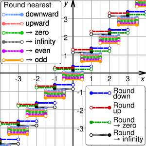
Graphs of the result, y, of rounding x using different methods. For clarity, the graphs are shown displaced from integer y values. In the SVG file, hover over a method to highlight it and, in SMIL-enabled browsers, click to select or deselect it.
Rounding means replacing a number with an approximate value that has a shorter, simpler, or more explicit representation. For example, replacing $23.4476 with $23.45, the fraction 312/937 with 1/3, or the expression √2 with 1.414.
Rounding is often done to obtain a value that is easier to report and communicate than the original. Rounding can also be important to avoid misleadingly precise reporting of a computed number, measurement, or estimate; for example, a quantity that was computed as 123,456 but is known to be accurate only to within a few hundred units is usually better stated as «about 123,500».
On the other hand, rounding of exact numbers will introduce some round-off error in the reported result. Rounding is almost unavoidable when reporting many computations – especially when dividing two numbers in integer or fixed-point arithmetic; when computing mathematical functions such as square roots, logarithms, and sines; or when using a floating-point representation with a fixed number of significant digits. In a sequence of calculations, these rounding errors generally accumulate, and in certain ill-conditioned cases they may make the result meaningless.
Accurate rounding of transcendental mathematical functions is difficult because the number of extra digits that need to be calculated to resolve whether to round up or down cannot be known in advance. This problem is known as «the table-maker’s dilemma».
Rounding has many similarities to the quantization that occurs when physical quantities must be encoded by numbers or digital signals.
A wavy equals sign (≈: approximately equal to) is sometimes used to indicate rounding of exact numbers, e.g., 9.98 ≈ 10. This sign was introduced by Alfred George Greenhill in 1892.[1]
Ideal characteristics of rounding methods include:
- Rounding should be done by a function. This way, when the same input is rounded in different instances, the output is unchanged.
- Calculations done with rounding should be close to those done without rounding.
- As a result of (1) and (2), the output from rounding should be close to its input, often as close as possible by some metric.
- To be considered rounding, the range will be a subset of the domain, in general discrete. A classical range is the integers, Z.
- Rounding should preserve symmetries that already exist between the domain and range. With finite precision (or a discrete domain), this translates to removing bias.
- A rounding method should have utility in computer science or human arithmetic where finite precision is used, and speed is a consideration.
Because it is not usually possible for a method to satisfy all ideal characteristics, many different rounding methods exist.
As a general rule, rounding is idempotent;[2] i.e., once a number has been rounded, rounding it again will not change its value. Rounding functions are also monotonic; i.e., rounding a larger number gives a larger or equal result than rounding a smaller number[clarification needed]. In the general case of a discrete range, they are piecewise constant functions.
Types of rounding[edit]
Typical rounding problems include:
| Rounding problem | Example input | Result | Rounding criterion |
|---|---|---|---|
| Approximating an irrational number by a fraction | π | 22 / 7 | 1-digit-denominator |
| Approximating a rational number by another fraction with smaller numerator and denominator | 399 / 941 | 3 / 7 | 1-digit-denominator |
| Approximating a fraction, which have periodic decimal expansion, by a finite decimal fraction | 5 / 3 | 1.6667 | 4 decimal places |
| Approximating a fractional decimal number by one with fewer digits | 2.1784 | 2.18 | 2 decimal places |
| Approximating a decimal integer by an integer with more trailing zeros | 23,217 | 23,200 | 3 significant figures |
| Approximating a large decimal integer using scientific notation | 300,999,999 | 3.01 × 10⁸ | 3 significant figures |
| Approximating a value by a multiple of a specified amount | 48.2 | 45 | Multiple of 15 |
| Rounding each one of a finite set of real numbers (mostly fractions) to an integer (sometimes the second-nearest integer) so that the sum of the rounded numbers equals the rounded sum of the numbers (needed e.g. [1] for the apportionment of seats, implemented e.g. by the largest remainder method, see Mathematics of apportionment, and [2] for distributing the total VAT of an invoice to its items) | {3/12, 4/12, 5/12} | {0, 0, 1} | Sum of rounded elements equals rounded sum of elements |
Rounding to integer[edit]
The most basic form of rounding is to replace an arbitrary number by an integer. All the following rounding modes are concrete implementations of an abstract single-argument «round()» procedure. These are true functions (with the exception of those that use randomness).
Directed rounding to an integer[edit]
These four methods are called directed rounding, as the displacements from the original number x to the rounded value y are all directed toward or away from the same limiting value (0, +∞, or −∞). Directed rounding is used in interval arithmetic and is often required in financial calculations.
If x is positive, round-down is the same as round-toward-zero, and round-up is the same as round-away-from-zero. If x is negative, round-down is the same as round-away-from-zero, and round-up is the same as round-toward-zero. In any case, if x is an integer, y is just x.
Where many calculations are done in sequence, the choice of rounding method can have a very significant effect on the result. A famous instance involved a new index set up by the Vancouver Stock Exchange in 1982. It was initially set at 1000.000 (three decimal places of accuracy), and after 22 months had fallen to about 520 — whereas stock prices had generally increased in the period. The problem was caused by the index being recalculated thousands of times daily, and always being rounded down to 3 decimal places, in such a way that the rounding errors accumulated. Recalculating with better rounding gave an index value of 1098.892 at the end of the same period.[3]
For the examples below, sgn(x) refers to the sign function applied to the original number, x.
Rounding down[edit]
- round down (or take the floor, or round toward negative infinity): y is the largest integer that does not exceed x.

For example, 23.7 gets rounded to 23, and −23.2 gets rounded to −24.
Rounding up[edit]
- round up (or take the ceiling, or round toward positive infinity): y is the smallest integer that is not less than x.

For example, 23.2 gets rounded to 24, and −23.7 gets rounded to −23.
Rounding toward zero[edit]
- round toward zero (or truncate, or round away from infinity): y is the integer that is closest to x such that it is between 0 and x (included); i.e. y is the integer part of x, without its fraction digits.

For example, 23.7 gets rounded to 23, and −23.7 gets rounded to −23.
Rounding away from zero[edit]
- round away from zero (or round toward infinity): y is the integer that is closest to 0 (or equivalently, to x) such that x is between 0 and y (included).

For example, 23.2 gets rounded to 24, and −23.2 gets rounded to −24.
Rounding to the nearest integer[edit]
Rounding a number x to the nearest integer requires some tie-breaking rule for those cases when x is exactly half-way between two integers — that is, when the fraction part of x is exactly 0.5.
If it were not for the 0.5 fractional parts, the round-off errors introduced by the round to nearest method would be symmetric: for every fraction that gets rounded down (such as 0.268), there is a complementary fraction (namely, 0.732) that gets rounded up by the same amount.
When rounding a large set of fixed-point numbers with uniformly distributed fractional parts, the rounding errors by all values, with the omission of those having 0.5 fractional part, would statistically compensate each other. This means that the expected (average) value of the rounded numbers is equal to the expected value of the original numbers when numbers with fractional part 0.5 from the set are removed.
In practice, floating-point numbers are typically used, which have even more computational nuances because they are not equally spaced.
Rounding half up[edit]
The following tie-breaking rule, called round half up (or round half toward positive infinity), is widely used in many disciplines.[citation needed] That is, half-way values of x are always rounded up.
- If the fractional part of x is exactly 0.5, then y = x + 0.5

For example, 23.5 gets rounded to 24, and −23.5 gets rounded to −23.
However, some programming languages (such as Java, Python) define their half up as round half away from zero here.[4][5]
This method only requires checking one digit to determine rounding direction in two’s complement and similar representations.
Rounding half down[edit]
One may also use round half down (or round half toward negative infinity) as opposed to the more common round half up.
- If the fractional part of x is exactly 0.5, then y = x − 0.5

For example, 23.5 gets rounded to 23, and −23.5 gets rounded to −24.
However, some programming languages (such as Java, Python) define their half down as round half toward zero here.[4][5]
Rounding half toward zero[edit]
One may also round half toward zero (or round half away from infinity) as opposed to the conventional round half away from zero.
- If the fractional part of x is exactly 0.5, then y = x − 0.5 if x is positive, and y = x + 0.5 if x is negative.

For example, 23.5 gets rounded to 23, and −23.5 gets rounded to −23.
This method treats positive and negative values symmetrically, and therefore is free of overall positive/negative bias if the original numbers are positive or negative with equal probability. It does, however, still have bias toward zero.
Rounding half away from zero[edit]
The other tie-breaking method commonly taught and used is the round half away from zero (or round half toward infinity), namely:
- If the fractional part of x is exactly 0.5, then y = x + 0.5 if x is positive, and y = x − 0.5 if x is negative.

For example, 23.5 gets rounded to 24, and −23.5 gets rounded to −24.
This can be more efficient on binary computers because only the first omitted bit needs to be considered to determine if it rounds up (on a 1) or down (on a 0). This is one method used when rounding to significant figures due to its simplicity.
This method, also known as commercial rounding,[citation needed] treats positive and negative values symmetrically, and therefore is free of overall positive/negative bias if the original numbers are positive or negative with equal probability. It does, however, still have bias away from zero.
It is often used for currency conversions and price roundings (when the amount is first converted into the smallest significant subdivision of the currency, such as cents of a euro) as it is easy to explain by just considering the first fractional digit, independently of supplementary precision digits or sign of the amount (for strict equivalence between the paying and recipient of the amount).
Rounding half to even[edit]
A tie-breaking rule without positive/negative bias and without bias toward/away from zero is round half to even. By this convention, if the fractional part of x is 0.5, then y is the even integer nearest to x. Thus, for example, +23.5 becomes +24, as does +24.5; however, −23.5 becomes −24, as does −24.5. This function minimizes the expected error when summing over rounded figures, even when the inputs are mostly positive or mostly negative, provided they are neither mostly even nor mostly odd.
This variant of the round-to-nearest method is also called convergent rounding, statistician’s rounding, Dutch rounding, Gaussian rounding, odd–even rounding,[6] or bankers’ rounding.
This is the default rounding mode used in IEEE 754 operations for results in binary floating-point formats, and the more sophisticated mode[clarification needed] used when rounding to significant figures.
By eliminating bias, repeated addition or subtraction of independent numbers, as in a one-dimensional random walk, will give a rounded result with an error that tends to grow in proportion to the square root of the number of operations rather than linearly.
However, this rule distorts the distribution by increasing the probability of evens relative to odds. Typically this is less important[citation needed] than the biases that are eliminated by this method.
Rounding half to odd[edit]
A similar tie-breaking rule to round half to even is round half to odd. In this approach, if the fractional part of x is 0.5, then y is the odd integer nearest to x. Thus, for example, +23.5 becomes +23, as does +22.5; while −23.5 becomes −23, as does −22.5.
This method is also free from positive/negative bias and bias toward/away from zero, provided the numbers to be rounded are neither mostly even nor mostly odd. It also shares the round half to even property of distorting the original distribution, as it increases the probability of odds relative to evens.
This variant is almost never used in computations, except in situations where one wants to avoid increasing the scale of floating-point numbers, which have a limited exponent range. With round half to even, a non-infinite number would round to infinity, and a small denormal value would round to a normal non-zero value. Effectively, this mode prefers preserving the existing scale of tie numbers, avoiding out-of-range results when possible for numeral systems of even radix (such as binary and decimal).[clarification needed (see talk)]
Rounding to prepare for shorter precision[edit]
This rounding mode (RPSP in this chapter) is used to avoid getting wrong result with double (including multiple) rounding. With this rounding mode, one can avoid wrong result after double rounding, if all roundings except the final one are done using RPSP, and only final rounding uses the externally requested mode.
With decimal arithmetic, if there is a choice between numbers with the smallest significant digit 0 or 1, 4 or 5, 5 or 6, 9 or 0, then the digit different from 0 or 5 shall be selected; otherwise, choice is arbitrary. IBM defines [7] that, in the latter case, a digit with the smaller magnitude shall be selected. RPSP can be applied with the step between two consequent roundings as small as a single digit (for example, rounding to 1/10 can be applied after rounding to 1/100).
For example, when rounding to integer,
- 20.0 is rounded to 20;
- 20.01, 20.1, 20.9, 20.99, 21, 21.01, 21.9, 21.99 are rounded to 21;
- 22.0, 22.1, 22.9, 22.99 are rounded to 22;
- 24.0, 24.1, 24.9, 24.99 are rounded to 24;
- 25.0 is rounded to 25;
- 25.01, 25.1 are rounded to 26.
In the example from «Double rounding» section, rounding 9.46 to one decimal gives 9.4, which rounding to integer in turn gives 9.
With binary arithmetic, the rounding is made as «round to odd» (not to be mixed with «round half to odd».) For example, when rounding to 1/4:
- x == 2.0 => result is 2
- 2.0 < x < 2.5 => result is 2.25
- x == 2.5 => result is 2.5
- 2.5 < x < 3.0 => result is 2.75
- x == 3.0 => result is 3.0
For correct results, RPSP shall be applied with the step of at least 2 binary digits, otherwise, wrong result may appear. For example,
- 3.125 RPSP to 1/4 => result is 3.25
- 3.25 RPSP to 1/2 => result is 3.5
- 3.5 round-half-to-even to 1 => result is 4 (wrong)
If the step is 2 bits or more, RPSP gives 3.25 which, in turn, round-half-to-even to integer results in 3.
RPSP is implemented in hardware in IBM zSeries and pSeries.
Randomized rounding to an integer[edit]
Alternating tie-breaking[edit]
One method, more obscure than most, is to alternate direction when rounding a number with 0.5 fractional part. All others are rounded to the closest integer.
- Whenever the fractional part is 0.5, alternate rounding up or down: for the first occurrence of a 0.5 fractional part, round up, for the second occurrence, round down, and so on. Alternatively, the first 0.5 fractional part rounding can be determined by a random seed. «Up» and «down» can be any two rounding methods that oppose each other — toward and away from positive infinity or toward and away from zero.
If occurrences of 0.5 fractional parts occur significantly more than a restart of the occurrence «counting», then it is effectively bias free. With guaranteed zero bias, it is useful if the numbers are to be summed or averaged.
Random tie-breaking[edit]
- If the fractional part of x is 0.5, choose y randomly between x + 0.5 and x − 0.5, with equal probability. All others are rounded to the closest integer.
Like round-half-to-even and round-half-to-odd, this rule is essentially free of overall bias, but it is also fair among even and odd y values. An advantage over alternate tie-breaking is that the last direction of rounding on the 0.5 fractional part does not have to be «remembered».
Stochastic rounding[edit]
Rounding as follows to one of the closest integer toward negative infinity and the closest integer toward positive infinity, with a probability dependent on the proximity is called stochastic rounding and will give an unbiased result on average.[8]

For example, 1.6 would be rounded to 1 with probability 0.4 and to 2 with probability 0.6.
Stochastic rounding can be accurate in a way that a rounding function can never be. For example, suppose one started with 0 and added 0.3 to that one hundred times while rounding the running total between every addition. The result would be 0 with regular rounding, but with stochastic rounding, the expected result would be 30, which is the same value obtained without rounding. This can be useful in machine learning where the training may use low precision arithmetic iteratively.[8] Stochastic rounding is also a way to achieve 1-dimensional dithering.
Comparison of approaches for rounding to an integer[edit]
| Value | Functional methods | Randomized methods | |||||||||||||||
|---|---|---|---|---|---|---|---|---|---|---|---|---|---|---|---|---|---|
| Directed rounding | Round to nearest | Round to prepare for shorter precision | Alternating tie-break | Random tie-break | Stochastic | ||||||||||||
| Down (toward −∞) |
Up (toward +∞) |
Toward 0 | Away From 0 | Half Down (toward −∞) |
Half Up (toward +∞) |
Half Toward 0 | Half Away From 0 | Half to Even | Half to Odd | Average | SD | Average | SD | Average | SD | ||
| +1.8 | +1 | +2 | +1 | +2 | +2 | +2 | +2 | +2 | +2 | +2 | +1 | +2 | 0 | +2 | 0 | +1.8 | 0.04 |
| +1.5 | +1 | +1 | +1 | +1.505 | 0 | +1.5 | 0.05 | +1.5 | 0.05 | ||||||||
| +1.2 | +1 | +1 | +1 | +1 | 0 | +1 | 0 | +1.2 | 0.04 | ||||||||
| +0.8 | 0 | +1 | 0 | +1 | +0.8 | 0.04 | |||||||||||
| +0.5 | 0 | 0 | 0 | +0.505 | 0 | +0.5 | 0.05 | +0.5 | 0.05 | ||||||||
| +0.2 | 0 | 0 | 0 | 0 | 0 | 0 | 0 | +0.2 | 0.04 | ||||||||
| −0.2 | −1 | 0 | −1 | −1 | −0.2 | 0.04 | |||||||||||
| −0.5 | −1 | −1 | −1 | −0.495 | 0 | −0.5 | 0.05 | −0.5 | 0.05 | ||||||||
| −0.8 | −1 | −1 | −1 | −1 | 0 | −1 | 0 | −0.8 | 0.04 | ||||||||
| −1.2 | −2 | −1 | −1 | −2 | −1.2 | 0.04 | |||||||||||
| −1.5 | −2 | −2 | −2 | −1.495 | 0 | −1.5 | 0.05 | −1.5 | 0.05 | ||||||||
| −1.8 | −2 | −2 | −2 | −2 | 0 | −2 | 0 | −1.8 | 0.04 |
Rounding to other values[edit]
Rounding to a specified multiple[edit]
The most common type of rounding is to round to an integer; or, more generally, to an integer multiple of some increment — such as rounding to whole tenths of seconds, hundredths of a dollar, to whole multiples of 1/2 or 1/8 inch, to whole dozens or thousands, etc.
In general, rounding a number x to a multiple of some specified positive value m entails the following steps:

For example, rounding x = 2.1784 dollars to whole cents (i.e., to a multiple of 0.01) entails computing 2.1784 / 0.01 = 217.84, then rounding that to 218, and finally computing 218 × 0.01 = 2.18.
When rounding to a predetermined number of significant digits, the increment m depends on the magnitude of the number to be rounded (or of the rounded result).
The increment m is normally a finite fraction in whatever numeral system is used to represent the numbers. For display to humans, that usually means the decimal numeral system (that is, m is an integer times a power of 10, like 1/1000 or 25/100). For intermediate values stored in digital computers, it often means the binary numeral system (m is an integer times a power of 2).
The abstract single-argument «round()» function that returns an integer from an arbitrary real value has at least a dozen distinct concrete definitions presented in the rounding to integer section. The abstract two-argument «roundToMultiple()» function is formally defined here, but in many cases it is used with the implicit value m = 1 for the increment and then reduces to the equivalent abstract single-argument function, with also the same dozen distinct concrete definitions.
Logarithmic rounding[edit]
Rounding to a specified power[edit]
Rounding to a specified power is very different from rounding to a specified multiple; for example, it is common in computing to need to round a number to a whole power of 2. The steps, in general, to round a positive number x to a power of some positive number b other than 1, are:

Many of the caveats applicable to rounding to a multiple are applicable to rounding to a power.
Scaled rounding[edit]
This type of rounding, which is also named rounding to a logarithmic scale, is a variant of rounding to a specified power. Rounding on a logarithmic scale is accomplished by taking the log of the amount and doing normal rounding to the nearest value on the log scale.
For example, resistors are supplied with preferred numbers on a logarithmic scale. In particular, for resistors with a 10% accuracy, they are supplied with nominal values 100, 120, 150, 180, 220, etc. rounded to multiples of 10 (E12 series). If a calculation indicates a resistor of 165 ohms is required then log(150) = 2.176, log(165) = 2.217 and log(180) = 2.255. The logarithm of 165 is closer to the logarithm of 180 therefore a 180 ohm resistor would be the first choice if there are no other considerations.
Whether a value x ∈ (a, b) rounds to a or b depends upon whether the squared value x2 is greater than or less than the product ab. The value 165 rounds to 180 in the resistors example because 1652 = 27225 is greater than 150 × 180 = 27000.
Floating-point rounding[edit]
In floating-point arithmetic, rounding aims to turn a given value x into a value y with a specified number of significant digits. In other words, y should be a multiple of a number m that depends on the magnitude of x. The number m is a power of the base (usually 2 or 10) of the floating-point representation.
Apart from this detail, all the variants of rounding discussed above apply to the rounding of floating-point numbers as well. The algorithm for such rounding is presented in the Scaled rounding section above, but with a constant scaling factor s = 1, and an integer base b > 1.
Where the rounded result would overflow the result for a directed rounding is either the appropriate signed infinity when «rounding away from zero», or the highest representable positive finite number (or the lowest representable negative finite number if x is negative), when «rounding toward zero». The result of an overflow for the usual case of round to nearest is always the appropriate infinity.
Rounding to a simple fraction[edit]
In some contexts it is desirable to round a given number x to a «neat» fraction — that is, the nearest fraction y = m/n whose numerator m and denominator n do not exceed a given maximum. This problem is fairly distinct from that of rounding a value to a fixed number of decimal or binary digits, or to a multiple of a given unit m. This problem is related to Farey sequences, the Stern–Brocot tree, and continued fractions.
Rounding to an available value[edit]
Finished lumber, writing paper, capacitors, and many other products are usually sold in only a few standard sizes.
Many design procedures describe how to calculate an approximate value, and then «round» to some standard size using phrases such as «round down to nearest standard value», «round up to nearest standard value», or «round to nearest standard value».[9][10]
When a set of preferred values is equally spaced on a logarithmic scale, choosing the closest preferred value to any given value can be seen as a form of scaled rounding. Such rounded values can be directly calculated.[11]
Rounding in other contexts[edit]
Dithering and error diffusion[edit]
When digitizing continuous signals, such as sound waves, the overall effect of a number of measurements is more important than the accuracy of each individual measurement. In these circumstances, dithering, and a related technique, error diffusion, are normally used. A related technique called pulse-width modulation is used to achieve analog type output from an inertial device by rapidly pulsing the power with a variable duty cycle.
Error diffusion tries to ensure the error, on average, is minimized. When dealing with a gentle slope from one to zero, the output would be zero for the first few terms until the sum of the error and the current value becomes greater than 0.5, in which case a 1 is output and the difference subtracted from the error so far. Floyd–Steinberg dithering is a popular error diffusion procedure when digitizing images.
As a one-dimensional example, suppose the numbers 0.9677, 0.9204, 0.7451, and 0.3091 occur in order and each is to be rounded to a multiple of 0.01. In this case the cumulative sums, 0.9677, 1.8881 = 0.9677 + 0.9204, 2.6332 = 0.9677 + 0.9204 + 0.7451, and 2.9423 = 0.9677 + 0.9204 + 0.7451 + 0.3091, are each rounded to a multiple of 0.01: 0.97, 1.89, 2.63, and 2.94. The first of these and the differences of adjacent values give the desired rounded values: 0.97, 0.92 = 1.89 − 0.97, 0.74 = 2.63 − 1.89, and 0.31 = 2.94 − 2.63.
Monte Carlo arithmetic[edit]
Monte Carlo arithmetic is a technique in Monte Carlo methods where the rounding is randomly up or down. Stochastic rounding can be used for Monte Carlo arithmetic, but in general, just rounding up or down with equal probability is more often used. Repeated runs will give a random distribution of results which can indicate the stability of the computation.[12]
Exact computation with rounded arithmetic[edit]
It is possible to use rounded arithmetic to evaluate the exact value of a function with integer domain and range. For example, if an integer n is known to be a perfect square, its square root can be computed by converting n to a floating-point value z, computing the approximate square root x of z with floating point, and then rounding x to the nearest integer y. If n is not too big, the floating-point round-off error in x will be less than 0.5, so the rounded value y will be the exact square root of n. This is essentially why slide rules could be used for exact arithmetic.
Double rounding[edit]
Rounding a number twice in succession to different levels of precision, with the latter precision being coarser, is not guaranteed to give the same result as rounding once to the final precision except in the case of directed rounding.[nb 1] For instance rounding 9.46 to one decimal gives 9.5, and then 10 when rounding to integer using rounding half to even, but would give 9 when rounded to integer directly. Borman and Chatfield[13] discuss the implications of double rounding when comparing data rounded to one decimal place to specification limits expressed using integers.
In Martinez v. Allstate and Sendejo v. Farmers, litigated between 1995 and 1997, the insurance companies argued that double rounding premiums was permissible and in fact required. The US courts ruled against the insurance companies and ordered them to adopt rules to ensure single rounding.[14]
Some computer languages and the IEEE 754-2008 standard dictate that in straightforward calculations the result should not be rounded twice. This has been a particular problem with Java as it is designed to be run identically on different machines, special programming tricks have had to be used to achieve this with x87 floating point.[15][16] The Java language was changed to allow different results where the difference does not matter and require a strictfp qualifier to be used when the results have to conform accurately; strict floating point has been restored in Java 17.[17]
In some algorithms, an intermediate result is computed in a larger precision, then must be rounded to the final precision. Double rounding can be avoided by choosing an adequate rounding for the intermediate computation. This consists in avoiding to round to midpoints for the final rounding (except when the midpoint is exact). In binary arithmetic, the idea is to round the result toward zero, and set the least significant bit to 1 if the rounded result is inexact; this rounding is called sticky rounding.[18] Equivalently, it consists in returning the intermediate result when it is exactly representable, and the nearest floating-point number with an odd significand otherwise; this is why it is also known as rounding to odd.[19][20] A concrete implementation of this approach, for binary and decimal arithmetic, is implemented as Rounding to prepare for shorter precision.
Table-maker’s dilemma[edit]
William M. Kahan coined the term «The Table-Maker’s Dilemma» for the unknown cost of rounding transcendental functions:
Nobody knows how much it would cost to compute yw correctly rounded for every two floating-point arguments at which it does not over/underflow. Instead, reputable math libraries compute elementary transcendental functions mostly within slightly more than half an ulp and almost always well within one ulp. Why can’t yw be rounded within half an ulp like SQRT? Because nobody knows how much computation it would cost… No general way exists to predict how many extra digits will have to be carried to compute a transcendental expression and round it correctly to some preassigned number of digits. Even the fact (if true) that a finite number of extra digits will ultimately suffice may be a deep theorem.[21]
The IEEE 754 floating-point standard guarantees that add, subtract, multiply, divide, fused multiply–add, square root, and floating-point remainder will give the correctly rounded result of the infinite-precision operation. No such guarantee was given in the 1985 standard for more complex functions and they are typically only accurate to within the last bit at best. However, the 2008 standard guarantees that conforming implementations will give correctly rounded results which respect the active rounding mode; implementation of the functions, however, is optional.
Using the Gelfond–Schneider theorem and Lindemann–Weierstrass theorem, many of the standard elementary functions can be proved to return transcendental results, except on some well-known arguments; therefore, from a theoretical point of view, it is always possible to correctly round such functions. However, for an implementation of such a function, determining a limit for a given precision on how accurate results need to be computed, before a correctly rounded result can be guaranteed, may demand a lot of computation time or may be out of reach.[22] In practice, when this limit is not known (or only a very large bound is known), some decision has to be made in the implementation (see below); but according to a probabilistic model, correct rounding can be satisfied with a very high probability when using an intermediate accuracy of up to twice the number of digits of the target format plus some small constant (after taking special cases into account).
Some programming packages offer correct rounding. The GNU MPFR package gives correctly rounded arbitrary precision results. Some other libraries implement elementary functions with correct rounding in double precision:
- IBM’s ml4j, which stands for Mathematical Library for Java, written by Abraham Ziv and Moshe Olshansky in 1999, correctly rounded to nearest only.[23][24] This library was claimed to be portable, but only binaries for PowerPC/AIX, SPARC/Solaris and x86/Windows NT were provided. According to its documentation, this library uses a first step with an accuracy a bit larger than double precision, a second step based on double-double arithmetic, and a third step with a 768-bit precision based on arrays of IEEE 754 double-precision floating-point numbers.
- IBM’s Accurate portable mathematical library (abbreviated as APMathLib or just MathLib),[25][26] also called libultim,[27] in rounding to nearest only. This library uses up to 768 bits of working precision. It was included in the GNU C Library in 2001,[28] but the «slow paths» (providing correct rounding) were removed from 2018 to 2021.
- Sun Microsystems’s libmcr, in the 4 rounding modes.[29] For the difficult cases, this library also uses multiple precision, and the number of words is increased by 2 each time the Table-maker’s dilemma occurs (with undefined behavior in the very unlikely event that some limit of the machine is reached).
- CRlibm, written in the old Arénaire team (LIP, ENS Lyon). It supports the 4 rounding modes and is proved, using the knowledge of the hardest-to-round cases.[30][31]
- The CORE-MATH project provides some correctly rounded functions in the 4 rounding modes, using the knowledge of the hardest-to-round cases.[32][33]
There exist computable numbers for which a rounded value can never be determined no matter how many digits are calculated. Specific instances cannot be given but this follows from the undecidability of the halting problem. For instance, if Goldbach’s conjecture is true but unprovable, then the result of rounding the following value up to the next integer cannot be determined: either 1+10−n where n is the first even number greater than 4 which is not the sum of two primes, or 1 if there is no such number. The rounded result is 2 if such a number n exists and 1 otherwise. The value before rounding can however be approximated to any given precision even if the conjecture is unprovable.
Interaction with string searches[edit]
Rounding can adversely affect a string search for a number. For example, π rounded to four digits is «3.1416» but a simple search for this string will not discover «3.14159» or any other value of π rounded to more than four digits. In contrast, truncation does not suffer from this problem; for example, a simple string search for «3.1415», which is π truncated to four digits, will discover values of π truncated to more than four digits.
History[edit]
The concept of rounding is very old, perhaps older than the concept of division itself. Some ancient clay tablets found in Mesopotamia contain tables with rounded values of reciprocals and square roots in base 60.[34]
Rounded approximations to π, the length of the year, and the length of the month are also ancient—see base 60 examples.
The round-to-even method has served as the ASTM (E-29) standard since 1940. The origin of the terms unbiased rounding and statistician’s rounding are fairly self-explanatory. In the 1906 fourth edition of Probability and Theory of Errors[35] Robert Simpson Woodward called this «the computer’s rule» indicating that it was then in common use by human computers who calculated mathematical tables. Churchill Eisenhart indicated the practice was already «well established» in data analysis by the 1940s.[36]
The origin of the term bankers’ rounding remains more obscure. If this rounding method was ever a standard in banking, the evidence has proved extremely difficult to find. To the contrary, section 2 of the European Commission report The Introduction of the Euro and the Rounding of Currency Amounts[37] suggests that there had previously been no standard approach to rounding in banking; and it specifies that «half-way» amounts should be rounded up.
Until the 1980s, the rounding method used in floating-point computer arithmetic was usually fixed by the hardware, poorly documented, inconsistent, and different for each brand and model of computer. This situation changed after the IEEE 754 floating-point standard was adopted by most computer manufacturers. The standard allows the user to choose among several rounding modes, and in each case specifies precisely how the results should be rounded. These features made numerical computations more predictable and machine-independent, and made possible the efficient and consistent implementation of interval arithmetic.
Currently, much research tends to round to multiples of 5 or 2. For example, Jörg Baten used age heaping in many studies, to evaluate the numeracy level of ancient populations. He came up with the ABCC Index, which enables the comparison of the numeracy among regions possible without any historical sources where the population literacy was measured.[38]
Rounding functions in programming languages[edit]
Most programming languages provide functions or special syntax to round fractional numbers in various ways. The earliest numeric languages, such as FORTRAN and C, would provide only one method, usually truncation (toward zero). This default method could be implied in certain contexts, such as when assigning a fractional number to an integer variable, or using a fractional number as an index of an array. Other kinds of rounding had to be programmed explicitly; for example, rounding a positive number to the nearest integer could be implemented by adding 0.5 and truncating.
In the last decades, however, the syntax and the standard libraries of most languages have commonly provided at least the four basic rounding functions (up, down, to nearest, and toward zero). The tie-breaking method can vary depending on the language and version or might be selectable by the programmer. Several languages follow the lead of the IEEE 754 floating-point standard, and define these functions as taking a double-precision float argument and returning the result of the same type, which then may be converted to an integer if necessary. This approach may avoid spurious overflows because floating-point types have a larger range than integer types. Some languages, such as PHP, provide functions that round a value to a specified number of decimal digits (e.g., from 4321.5678 to 4321.57 or 4300). In addition, many languages provide a printf or similar string formatting function, which allows one to convert a fractional number to a string, rounded to a user-specified number of decimal places (the precision). On the other hand, truncation (round to zero) is still the default rounding method used by many languages, especially for the division of two integer values.
In contrast, CSS and SVG do not define any specific maximum precision for numbers and measurements, which they treat and expose in their DOM and in their IDL interface as strings as if they had infinite precision, and do not discriminate between integers and floating-point values; however, the implementations of these languages will typically convert these numbers into IEEE 754 double-precision floating-point values before exposing the computed digits with a limited precision (notably within standard JavaScript or ECMAScript[39] interface bindings).
Other rounding standards[edit]
Some disciplines or institutions have issued standards or directives for rounding.
US weather observations[edit]
In a guideline issued in mid-1966,[40] the U.S. Office of the Federal Coordinator for Meteorology determined that weather data should be rounded to the nearest round number, with the «round half up» tie-breaking rule. For example, 1.5 rounded to integer should become 2, and −1.5 should become −1. Prior to that date, the tie-breaking rule was «round half away from zero».
Negative zero in meteorology[edit]
Some meteorologists may write «−0» to indicate a temperature between 0.0 and −0.5 degrees (exclusive) that was rounded to an integer. This notation is used when the negative sign is considered important, no matter how small is the magnitude; for example, when rounding temperatures in the Celsius scale, where below zero indicates freezing.[citation needed]
See also[edit]
- Cash rounding, dealing with the absence of extremely low-value coins
- Data binning, a similar operation
- Gal’s accurate tables
- Interval arithmetic
- ISO/IEC 80000
- Kahan summation algorithm
- Party-list proportional representation, an application of rounding to integers that has been thoroughly investigated
- Signed-digit representation
- Truncation
Notes[edit]
- ^ A case where double rounding always leads to the same value as directly rounding to the final precision is when the radix is odd.
References[edit]
- ^ Isaiah Lankham, Bruno Nachtergaele, Anne Schilling: Linear Algebra as an Introduction to Abstract Mathematics. World Scientific, Singapur 2016, ISBN 978-981-4730-35-8, p. 186.
- ^ Kulisch, Ulrich W. (July 1977). «Mathematical foundation of computer arithmetic». IEEE Transactions on Computers. C-26 (7): 610–621. doi:10.1109/TC.1977.1674893. S2CID 35883481.
- ^ Higham, Nicholas John (2002). Accuracy and stability of numerical algorithms. p. 54. ISBN 978-0-89871-521-7.
- ^ a b «java.math.RoundingMode». Oracle.
- ^ a b «decimal — Decimal fixed point and floating point arithmetic». Python Software Foundation.
- ^ Engineering Drafting Standards Manual (NASA), X-673-64-1F, p90
- ^ IBM z/Architecture Principles of Operation
- ^ a b Gupta, Suyog; Angrawl, Ankur; Gopalakrishnan, Kailash; Narayanan, Pritish (2016-02-09). «Deep Learning with Limited Numerical Precision». p. 3. arXiv:1502.02551 [cs.LG].
- ^ «Zener Diode Voltage Regulators» (PDF). Archived (PDF) from the original on 2011-07-13. Retrieved 2010-11-24.
- ^ «Build a Mirror Tester»
- ^ Bruce Trump, Christine Schneider.
«Excel Formula Calculates Standard 1%-Resistor Values». Electronic Design, 2002-01-21. [1] - ^ Parker, D. Stott; Eggert, Paul R.; Pierce, Brad (2000-03-28). «Monte Carlo Arithmetic: a framework for the statistical analysis of roundoff errors». IEEE Computation in Science and Engineering.
- ^ Borman, Phil; Chatfield, Marion (2015-11-10). «Avoid the perils of using rounded data». Journal of Pharmaceutical and Biomedical Analysis. 115: 506–507. doi:10.1016/j.jpba.2015.07.021. PMID 26299526.
- ^ Deborah R. Hensler (2000). Class Action Dilemmas: Pursuing Public Goals for Private Gain. RAND. pp. 255–293. ISBN 0-8330-2601-1.
- ^ Samuel A. Figueroa (July 1995). «When is double rounding innocuous?». ACM SIGNUM Newsletter. ACM. 30 (3): 21–25. doi:10.1145/221332.221334. S2CID 14829295.
- ^ Roger Golliver (October 1998). «Efficiently producing default orthogonal IEEE double results using extended IEEE hardware» (PDF). Intel.
- ^ Darcy, Joseph D. «JEP 306: Restore Always-Strict Floating-Point Semantics». Retrieved 2021-09-12.
- ^ Moore, J. Strother; Lynch, Tom; Kaufmann, Matt (1996). «A mechanically checked proof of the correctness of the kernel of the AMD5K86 floating-point division algorithm» (PDF). IEEE Transactions on Computers. 47. CiteSeerX 10.1.1.43.3309. doi:10.1109/12.713311. Retrieved 2016-08-02.
- ^ Boldo, Sylvie; Melquiond, Guillaume (2008). «Emulation of a FMA and correctly-rounded sums: proved algorithms using rounding to odd» (PDF). IEEE Transactions on Computers. 57 (4): 462–471. doi:10.1109/TC.2007.70819. S2CID 1850330. Retrieved 2016-08-02.
- ^ «21718 – real.c rounding not perfect». gcc.gnu.org.
- ^ Kahan, William Morton. «A Logarithm Too Clever by Half». Retrieved 2008-11-14.
- ^ Muller, Jean-Michel; Brisebarre, Nicolas; de Dinechin, Florent; Jeannerod, Claude-Pierre; Lefèvre, Vincent; Melquiond, Guillaume; Revol, Nathalie; Stehlé, Damien; Torres, Serge (2010). «Chapter 12: Solving the Table Maker’s Dilemma». Handbook of Floating-Point Arithmetic (1 ed.). Birkhäuser. doi:10.1007/978-0-8176-4705-6. ISBN 978-0-8176-4704-9. LCCN 2009939668.
- ^ «NA Digest Sunday, April 18, 1999 Volume 99 : Issue 16». 1999-04-18. Retrieved 2022-08-29.
- ^ «Math Library for Java». Archived from the original on 1999-05-08.
- ^ «Accurate Portable Mathematical Library». Archived from the original on 2005-02-07.
- ^ mathlib on GitHub.
- ^ «libultim – ultimate correctly-rounded elementary-function library». Archived from the original on 2021-03-01.
- ^ «Git — glibc.git/commit». Sourceware.org. Retrieved 2022-07-18.
- ^ «libmcr – correctly-rounded elementary-function library».
- ^ «CRlibm – Correctly Rounded mathematical library». Archived from the original on 2016-10-27.
- ^ crlibm on GitHub
- ^ «The CORE-MATH project». Retrieved 2022-08-30.
- ^ Sibidanov, Alexei; Zimmermann, Paul; Glondu, Stéphane (2022). The CORE-MATH Project. 29th IEEE Symposium on Computer Arithmetic (ARITH 2022). Retrieved 2022-08-30.
- ^ Duncan J. Melville. «YBC 7289 clay tablet». 2006
- ^ Probability and theory of errors. historical.library.cornell.edu. Mathematical monographs, no. 7. J. Wiley & Son. 1906.
- ^ Churchill Eisenhart (1947). «Effects of Rounding or Grouping Data». In Eisenhart; Hastay; Wallis (eds.). Selected Techniques of Statistical Analysis for Scientific and Industrial Research, and Production and Management Engineering. New York: McGraw-Hill. pp. 187–223. Retrieved 2014-01-30.
- ^ «The Introduction of the Euro and the Rounding of Currency Amounts» (PDF). Archived (PDF) from the original on 2010-10-09. Retrieved 2011-08-19.
- ^ Baten, Jörg (2009). «Quantifying Quantitative Literacy: Age Heaping and the History of Human Capital» (PDF). Journal of Economic History. 69 (3): 783–808. doi:10.1017/S0022050709001120. hdl:10230/481. S2CID 35494384.
- ^ «ECMA-262 ECMAScript Language Specification» (PDF). ecma-international.org.
- ^ OFCM, 2005: Federal Meteorological Handbook No. 1 Archived 1999-04-20 at the Wayback Machine, Washington, DC., 104 pp.
External links[edit]
- Weisstein, Eric W. «Rounding». MathWorld.
- An introduction to different rounding algorithms that is accessible to a general audience but especially useful to those studying computer science and electronics.
- How To Implement Custom Rounding Procedures by Microsoft (broken)
Graphs of the result, y, of rounding x using different methods. For clarity, the graphs are shown displaced from integer y values. In the SVG file, hover over a method to highlight it and, in SMIL-enabled browsers, click to select or deselect it.
Rounding means replacing a number with an approximate value that has a shorter, simpler, or more explicit representation. For example, replacing $23.4476 with $23.45, the fraction 312/937 with 1/3, or the expression √2 with 1.414.
Rounding is often done to obtain a value that is easier to report and communicate than the original. Rounding can also be important to avoid misleadingly precise reporting of a computed number, measurement, or estimate; for example, a quantity that was computed as 123,456 but is known to be accurate only to within a few hundred units is usually better stated as «about 123,500».
On the other hand, rounding of exact numbers will introduce some round-off error in the reported result. Rounding is almost unavoidable when reporting many computations – especially when dividing two numbers in integer or fixed-point arithmetic; when computing mathematical functions such as square roots, logarithms, and sines; or when using a floating-point representation with a fixed number of significant digits. In a sequence of calculations, these rounding errors generally accumulate, and in certain ill-conditioned cases they may make the result meaningless.
Accurate rounding of transcendental mathematical functions is difficult because the number of extra digits that need to be calculated to resolve whether to round up or down cannot be known in advance. This problem is known as «the table-maker’s dilemma».
Rounding has many similarities to the quantization that occurs when physical quantities must be encoded by numbers or digital signals.
A wavy equals sign (≈: approximately equal to) is sometimes used to indicate rounding of exact numbers, e.g., 9.98 ≈ 10. This sign was introduced by Alfred George Greenhill in 1892.[1]
Ideal characteristics of rounding methods include:
- Rounding should be done by a function. This way, when the same input is rounded in different instances, the output is unchanged.
- Calculations done with rounding should be close to those done without rounding.
- As a result of (1) and (2), the output from rounding should be close to its input, often as close as possible by some metric.
- To be considered rounding, the range will be a subset of the domain, in general discrete. A classical range is the integers, Z.
- Rounding should preserve symmetries that already exist between the domain and range. With finite precision (or a discrete domain), this translates to removing bias.
- A rounding method should have utility in computer science or human arithmetic where finite precision is used, and speed is a consideration.
Because it is not usually possible for a method to satisfy all ideal characteristics, many different rounding methods exist.
As a general rule, rounding is idempotent;[2] i.e., once a number has been rounded, rounding it again will not change its value. Rounding functions are also monotonic; i.e., rounding a larger number gives a larger or equal result than rounding a smaller number[clarification needed]. In the general case of a discrete range, they are piecewise constant functions.
Types of rounding[edit]
Typical rounding problems include:
| Rounding problem | Example input | Result | Rounding criterion |
|---|---|---|---|
| Approximating an irrational number by a fraction | π | 22 / 7 | 1-digit-denominator |
| Approximating a rational number by another fraction with smaller numerator and denominator | 399 / 941 | 3 / 7 | 1-digit-denominator |
| Approximating a fraction, which have periodic decimal expansion, by a finite decimal fraction | 5 / 3 | 1.6667 | 4 decimal places |
| Approximating a fractional decimal number by one with fewer digits | 2.1784 | 2.18 | 2 decimal places |
| Approximating a decimal integer by an integer with more trailing zeros | 23,217 | 23,200 | 3 significant figures |
| Approximating a large decimal integer using scientific notation | 300,999,999 | 3.01 × 10⁸ | 3 significant figures |
| Approximating a value by a multiple of a specified amount | 48.2 | 45 | Multiple of 15 |
| Rounding each one of a finite set of real numbers (mostly fractions) to an integer (sometimes the second-nearest integer) so that the sum of the rounded numbers equals the rounded sum of the numbers (needed e.g. [1] for the apportionment of seats, implemented e.g. by the largest remainder method, see Mathematics of apportionment, and [2] for distributing the total VAT of an invoice to its items) | {3/12, 4/12, 5/12} | {0, 0, 1} | Sum of rounded elements equals rounded sum of elements |
Rounding to integer[edit]
The most basic form of rounding is to replace an arbitrary number by an integer. All the following rounding modes are concrete implementations of an abstract single-argument «round()» procedure. These are true functions (with the exception of those that use randomness).
Directed rounding to an integer[edit]
These four methods are called directed rounding, as the displacements from the original number x to the rounded value y are all directed toward or away from the same limiting value (0, +∞, or −∞). Directed rounding is used in interval arithmetic and is often required in financial calculations.
If x is positive, round-down is the same as round-toward-zero, and round-up is the same as round-away-from-zero. If x is negative, round-down is the same as round-away-from-zero, and round-up is the same as round-toward-zero. In any case, if x is an integer, y is just x.
Where many calculations are done in sequence, the choice of rounding method can have a very significant effect on the result. A famous instance involved a new index set up by the Vancouver Stock Exchange in 1982. It was initially set at 1000.000 (three decimal places of accuracy), and after 22 months had fallen to about 520 — whereas stock prices had generally increased in the period. The problem was caused by the index being recalculated thousands of times daily, and always being rounded down to 3 decimal places, in such a way that the rounding errors accumulated. Recalculating with better rounding gave an index value of 1098.892 at the end of the same period.[3]
For the examples below, sgn(x) refers to the sign function applied to the original number, x.
Rounding down[edit]
- round down (or take the floor, or round toward negative infinity): y is the largest integer that does not exceed x.
For example, 23.7 gets rounded to 23, and −23.2 gets rounded to −24.
Rounding up[edit]
- round up (or take the ceiling, or round toward positive infinity): y is the smallest integer that is not less than x.
For example, 23.2 gets rounded to 24, and −23.7 gets rounded to −23.
Rounding toward zero[edit]
- round toward zero (or truncate, or round away from infinity): y is the integer that is closest to x such that it is between 0 and x (included); i.e. y is the integer part of x, without its fraction digits.
For example, 23.7 gets rounded to 23, and −23.7 gets rounded to −23.
Rounding away from zero[edit]
- round away from zero (or round toward infinity): y is the integer that is closest to 0 (or equivalently, to x) such that x is between 0 and y (included).
For example, 23.2 gets rounded to 24, and −23.2 gets rounded to −24.
Rounding to the nearest integer[edit]
Rounding a number x to the nearest integer requires some tie-breaking rule for those cases when x is exactly half-way between two integers — that is, when the fraction part of x is exactly 0.5.
If it were not for the 0.5 fractional parts, the round-off errors introduced by the round to nearest method would be symmetric: for every fraction that gets rounded down (such as 0.268), there is a complementary fraction (namely, 0.732) that gets rounded up by the same amount.
When rounding a large set of fixed-point numbers with uniformly distributed fractional parts, the rounding errors by all values, with the omission of those having 0.5 fractional part, would statistically compensate each other. This means that the expected (average) value of the rounded numbers is equal to the expected value of the original numbers when numbers with fractional part 0.5 from the set are removed.
In practice, floating-point numbers are typically used, which have even more computational nuances because they are not equally spaced.
Rounding half up[edit]
The following tie-breaking rule, called round half up (or round half toward positive infinity), is widely used in many disciplines.[citation needed] That is, half-way values of x are always rounded up.
- If the fractional part of x is exactly 0.5, then y = x + 0.5
For example, 23.5 gets rounded to 24, and −23.5 gets rounded to −23.
However, some programming languages (such as Java, Python) define their half up as round half away from zero here.[4][5]
This method only requires checking one digit to determine rounding direction in two’s complement and similar representations.
Rounding half down[edit]
One may also use round half down (or round half toward negative infinity) as opposed to the more common round half up.
- If the fractional part of x is exactly 0.5, then y = x − 0.5
For example, 23.5 gets rounded to 23, and −23.5 gets rounded to −24.
However, some programming languages (such as Java, Python) define their half down as round half toward zero here.[4][5]
Rounding half toward zero[edit]
One may also round half toward zero (or round half away from infinity) as opposed to the conventional round half away from zero.
- If the fractional part of x is exactly 0.5, then y = x − 0.5 if x is positive, and y = x + 0.5 if x is negative.
For example, 23.5 gets rounded to 23, and −23.5 gets rounded to −23.
This method treats positive and negative values symmetrically, and therefore is free of overall positive/negative bias if the original numbers are positive or negative with equal probability. It does, however, still have bias toward zero.
Rounding half away from zero[edit]
The other tie-breaking method commonly taught and used is the round half away from zero (or round half toward infinity), namely:
- If the fractional part of x is exactly 0.5, then y = x + 0.5 if x is positive, and y = x − 0.5 if x is negative.
For example, 23.5 gets rounded to 24, and −23.5 gets rounded to −24.
This can be more efficient on binary computers because only the first omitted bit needs to be considered to determine if it rounds up (on a 1) or down (on a 0). This is one method used when rounding to significant figures due to its simplicity.
This method, also known as commercial rounding,[citation needed] treats positive and negative values symmetrically, and therefore is free of overall positive/negative bias if the original numbers are positive or negative with equal probability. It does, however, still have bias away from zero.
It is often used for currency conversions and price roundings (when the amount is first converted into the smallest significant subdivision of the currency, such as cents of a euro) as it is easy to explain by just considering the first fractional digit, independently of supplementary precision digits or sign of the amount (for strict equivalence between the paying and recipient of the amount).
Rounding half to even[edit]
A tie-breaking rule without positive/negative bias and without bias toward/away from zero is round half to even. By this convention, if the fractional part of x is 0.5, then y is the even integer nearest to x. Thus, for example, +23.5 becomes +24, as does +24.5; however, −23.5 becomes −24, as does −24.5. This function minimizes the expected error when summing over rounded figures, even when the inputs are mostly positive or mostly negative, provided they are neither mostly even nor mostly odd.
This variant of the round-to-nearest method is also called convergent rounding, statistician’s rounding, Dutch rounding, Gaussian rounding, odd–even rounding,[6] or bankers’ rounding.
This is the default rounding mode used in IEEE 754 operations for results in binary floating-point formats, and the more sophisticated mode[clarification needed] used when rounding to significant figures.
By eliminating bias, repeated addition or subtraction of independent numbers, as in a one-dimensional random walk, will give a rounded result with an error that tends to grow in proportion to the square root of the number of operations rather than linearly.
However, this rule distorts the distribution by increasing the probability of evens relative to odds. Typically this is less important[citation needed] than the biases that are eliminated by this method.
Rounding half to odd[edit]
A similar tie-breaking rule to round half to even is round half to odd. In this approach, if the fractional part of x is 0.5, then y is the odd integer nearest to x. Thus, for example, +23.5 becomes +23, as does +22.5; while −23.5 becomes −23, as does −22.5.
This method is also free from positive/negative bias and bias toward/away from zero, provided the numbers to be rounded are neither mostly even nor mostly odd. It also shares the round half to even property of distorting the original distribution, as it increases the probability of odds relative to evens.
This variant is almost never used in computations, except in situations where one wants to avoid increasing the scale of floating-point numbers, which have a limited exponent range. With round half to even, a non-infinite number would round to infinity, and a small denormal value would round to a normal non-zero value. Effectively, this mode prefers preserving the existing scale of tie numbers, avoiding out-of-range results when possible for numeral systems of even radix (such as binary and decimal).[clarification needed (see talk)]
Rounding to prepare for shorter precision[edit]
This rounding mode (RPSP in this chapter) is used to avoid getting wrong result with double (including multiple) rounding. With this rounding mode, one can avoid wrong result after double rounding, if all roundings except the final one are done using RPSP, and only final rounding uses the externally requested mode.
With decimal arithmetic, if there is a choice between numbers with the smallest significant digit 0 or 1, 4 or 5, 5 or 6, 9 or 0, then the digit different from 0 or 5 shall be selected; otherwise, choice is arbitrary. IBM defines [7] that, in the latter case, a digit with the smaller magnitude shall be selected. RPSP can be applied with the step between two consequent roundings as small as a single digit (for example, rounding to 1/10 can be applied after rounding to 1/100).
For example, when rounding to integer,
- 20.0 is rounded to 20;
- 20.01, 20.1, 20.9, 20.99, 21, 21.01, 21.9, 21.99 are rounded to 21;
- 22.0, 22.1, 22.9, 22.99 are rounded to 22;
- 24.0, 24.1, 24.9, 24.99 are rounded to 24;
- 25.0 is rounded to 25;
- 25.01, 25.1 are rounded to 26.
In the example from «Double rounding» section, rounding 9.46 to one decimal gives 9.4, which rounding to integer in turn gives 9.
With binary arithmetic, the rounding is made as «round to odd» (not to be mixed with «round half to odd».) For example, when rounding to 1/4:
- x == 2.0 => result is 2
- 2.0 < x < 2.5 => result is 2.25
- x == 2.5 => result is 2.5
- 2.5 < x < 3.0 => result is 2.75
- x == 3.0 => result is 3.0
For correct results, RPSP shall be applied with the step of at least 2 binary digits, otherwise, wrong result may appear. For example,
- 3.125 RPSP to 1/4 => result is 3.25
- 3.25 RPSP to 1/2 => result is 3.5
- 3.5 round-half-to-even to 1 => result is 4 (wrong)
If the step is 2 bits or more, RPSP gives 3.25 which, in turn, round-half-to-even to integer results in 3.
RPSP is implemented in hardware in IBM zSeries and pSeries.
Randomized rounding to an integer[edit]
Alternating tie-breaking[edit]
One method, more obscure than most, is to alternate direction when rounding a number with 0.5 fractional part. All others are rounded to the closest integer.
- Whenever the fractional part is 0.5, alternate rounding up or down: for the first occurrence of a 0.5 fractional part, round up, for the second occurrence, round down, and so on. Alternatively, the first 0.5 fractional part rounding can be determined by a random seed. «Up» and «down» can be any two rounding methods that oppose each other — toward and away from positive infinity or toward and away from zero.
If occurrences of 0.5 fractional parts occur significantly more than a restart of the occurrence «counting», then it is effectively bias free. With guaranteed zero bias, it is useful if the numbers are to be summed or averaged.
Random tie-breaking[edit]
- If the fractional part of x is 0.5, choose y randomly between x + 0.5 and x − 0.5, with equal probability. All others are rounded to the closest integer.
Like round-half-to-even and round-half-to-odd, this rule is essentially free of overall bias, but it is also fair among even and odd y values. An advantage over alternate tie-breaking is that the last direction of rounding on the 0.5 fractional part does not have to be «remembered».
Stochastic rounding[edit]
Rounding as follows to one of the closest integer toward negative infinity and the closest integer toward positive infinity, with a probability dependent on the proximity is called stochastic rounding and will give an unbiased result on average.[8]
For example, 1.6 would be rounded to 1 with probability 0.4 and to 2 with probability 0.6.
Stochastic rounding can be accurate in a way that a rounding function can never be. For example, suppose one started with 0 and added 0.3 to that one hundred times while rounding the running total between every addition. The result would be 0 with regular rounding, but with stochastic rounding, the expected result would be 30, which is the same value obtained without rounding. This can be useful in machine learning where the training may use low precision arithmetic iteratively.[8] Stochastic rounding is also a way to achieve 1-dimensional dithering.
Comparison of approaches for rounding to an integer[edit]
| Value | Functional methods | Randomized methods | |||||||||||||||
|---|---|---|---|---|---|---|---|---|---|---|---|---|---|---|---|---|---|
| Directed rounding | Round to nearest | Round to prepare for shorter precision | Alternating tie-break | Random tie-break | Stochastic | ||||||||||||
| Down (toward −∞) |
Up (toward +∞) |
Toward 0 | Away From 0 | Half Down (toward −∞) |
Half Up (toward +∞) |
Half Toward 0 | Half Away From 0 | Half to Even | Half to Odd | Average | SD | Average | SD | Average | SD | ||
| +1.8 | +1 | +2 | +1 | +2 | +2 | +2 | +2 | +2 | +2 | +2 | +1 | +2 | 0 | +2 | 0 | +1.8 | 0.04 |
| +1.5 | +1 | +1 | +1 | +1.505 | 0 | +1.5 | 0.05 | +1.5 | 0.05 | ||||||||
| +1.2 | +1 | +1 | +1 | +1 | 0 | +1 | 0 | +1.2 | 0.04 | ||||||||
| +0.8 | 0 | +1 | 0 | +1 | +0.8 | 0.04 | |||||||||||
| +0.5 | 0 | 0 | 0 | +0.505 | 0 | +0.5 | 0.05 | +0.5 | 0.05 | ||||||||
| +0.2 | 0 | 0 | 0 | 0 | 0 | 0 | 0 | +0.2 | 0.04 | ||||||||
| −0.2 | −1 | 0 | −1 | −1 | −0.2 | 0.04 | |||||||||||
| −0.5 | −1 | −1 | −1 | −0.495 | 0 | −0.5 | 0.05 | −0.5 | 0.05 | ||||||||
| −0.8 | −1 | −1 | −1 | −1 | 0 | −1 | 0 | −0.8 | 0.04 | ||||||||
| −1.2 | −2 | −1 | −1 | −2 | −1.2 | 0.04 | |||||||||||
| −1.5 | −2 | −2 | −2 | −1.495 | 0 | −1.5 | 0.05 | −1.5 | 0.05 | ||||||||
| −1.8 | −2 | −2 | −2 | −2 | 0 | −2 | 0 | −1.8 | 0.04 |
Rounding to other values[edit]
Rounding to a specified multiple[edit]
The most common type of rounding is to round to an integer; or, more generally, to an integer multiple of some increment — such as rounding to whole tenths of seconds, hundredths of a dollar, to whole multiples of 1/2 or 1/8 inch, to whole dozens or thousands, etc.
In general, rounding a number x to a multiple of some specified positive value m entails the following steps:
For example, rounding x = 2.1784 dollars to whole cents (i.e., to a multiple of 0.01) entails computing 2.1784 / 0.01 = 217.84, then rounding that to 218, and finally computing 218 × 0.01 = 2.18.
When rounding to a predetermined number of significant digits, the increment m depends on the magnitude of the number to be rounded (or of the rounded result).
The increment m is normally a finite fraction in whatever numeral system is used to represent the numbers. For display to humans, that usually means the decimal numeral system (that is, m is an integer times a power of 10, like 1/1000 or 25/100). For intermediate values stored in digital computers, it often means the binary numeral system (m is an integer times a power of 2).
The abstract single-argument «round()» function that returns an integer from an arbitrary real value has at least a dozen distinct concrete definitions presented in the rounding to integer section. The abstract two-argument «roundToMultiple()» function is formally defined here, but in many cases it is used with the implicit value m = 1 for the increment and then reduces to the equivalent abstract single-argument function, with also the same dozen distinct concrete definitions.
Logarithmic rounding[edit]
Rounding to a specified power[edit]
Rounding to a specified power is very different from rounding to a specified multiple; for example, it is common in computing to need to round a number to a whole power of 2. The steps, in general, to round a positive number x to a power of some positive number b other than 1, are:
Many of the caveats applicable to rounding to a multiple are applicable to rounding to a power.
Scaled rounding[edit]
This type of rounding, which is also named rounding to a logarithmic scale, is a variant of rounding to a specified power. Rounding on a logarithmic scale is accomplished by taking the log of the amount and doing normal rounding to the nearest value on the log scale.
For example, resistors are supplied with preferred numbers on a logarithmic scale. In particular, for resistors with a 10% accuracy, they are supplied with nominal values 100, 120, 150, 180, 220, etc. rounded to multiples of 10 (E12 series). If a calculation indicates a resistor of 165 ohms is required then log(150) = 2.176, log(165) = 2.217 and log(180) = 2.255. The logarithm of 165 is closer to the logarithm of 180 therefore a 180 ohm resistor would be the first choice if there are no other considerations.
Whether a value x ∈ (a, b) rounds to a or b depends upon whether the squared value x2 is greater than or less than the product ab. The value 165 rounds to 180 in the resistors example because 1652 = 27225 is greater than 150 × 180 = 27000.
Floating-point rounding[edit]
In floating-point arithmetic, rounding aims to turn a given value x into a value y with a specified number of significant digits. In other words, y should be a multiple of a number m that depends on the magnitude of x. The number m is a power of the base (usually 2 or 10) of the floating-point representation.
Apart from this detail, all the variants of rounding discussed above apply to the rounding of floating-point numbers as well. The algorithm for such rounding is presented in the Scaled rounding section above, but with a constant scaling factor s = 1, and an integer base b > 1.
Where the rounded result would overflow the result for a directed rounding is either the appropriate signed infinity when «rounding away from zero», or the highest representable positive finite number (or the lowest representable negative finite number if x is negative), when «rounding toward zero». The result of an overflow for the usual case of round to nearest is always the appropriate infinity.
Rounding to a simple fraction[edit]
In some contexts it is desirable to round a given number x to a «neat» fraction — that is, the nearest fraction y = m/n whose numerator m and denominator n do not exceed a given maximum. This problem is fairly distinct from that of rounding a value to a fixed number of decimal or binary digits, or to a multiple of a given unit m. This problem is related to Farey sequences, the Stern–Brocot tree, and continued fractions.
Rounding to an available value[edit]
Finished lumber, writing paper, capacitors, and many other products are usually sold in only a few standard sizes.
Many design procedures describe how to calculate an approximate value, and then «round» to some standard size using phrases such as «round down to nearest standard value», «round up to nearest standard value», or «round to nearest standard value».[9][10]
When a set of preferred values is equally spaced on a logarithmic scale, choosing the closest preferred value to any given value can be seen as a form of scaled rounding. Such rounded values can be directly calculated.[11]
Rounding in other contexts[edit]
Dithering and error diffusion[edit]
When digitizing continuous signals, such as sound waves, the overall effect of a number of measurements is more important than the accuracy of each individual measurement. In these circumstances, dithering, and a related technique, error diffusion, are normally used. A related technique called pulse-width modulation is used to achieve analog type output from an inertial device by rapidly pulsing the power with a variable duty cycle.
Error diffusion tries to ensure the error, on average, is minimized. When dealing with a gentle slope from one to zero, the output would be zero for the first few terms until the sum of the error and the current value becomes greater than 0.5, in which case a 1 is output and the difference subtracted from the error so far. Floyd–Steinberg dithering is a popular error diffusion procedure when digitizing images.
As a one-dimensional example, suppose the numbers 0.9677, 0.9204, 0.7451, and 0.3091 occur in order and each is to be rounded to a multiple of 0.01. In this case the cumulative sums, 0.9677, 1.8881 = 0.9677 + 0.9204, 2.6332 = 0.9677 + 0.9204 + 0.7451, and 2.9423 = 0.9677 + 0.9204 + 0.7451 + 0.3091, are each rounded to a multiple of 0.01: 0.97, 1.89, 2.63, and 2.94. The first of these and the differences of adjacent values give the desired rounded values: 0.97, 0.92 = 1.89 − 0.97, 0.74 = 2.63 − 1.89, and 0.31 = 2.94 − 2.63.
Monte Carlo arithmetic[edit]
Monte Carlo arithmetic is a technique in Monte Carlo methods where the rounding is randomly up or down. Stochastic rounding can be used for Monte Carlo arithmetic, but in general, just rounding up or down with equal probability is more often used. Repeated runs will give a random distribution of results which can indicate the stability of the computation.[12]
Exact computation with rounded arithmetic[edit]
It is possible to use rounded arithmetic to evaluate the exact value of a function with integer domain and range. For example, if an integer n is known to be a perfect square, its square root can be computed by converting n to a floating-point value z, computing the approximate square root x of z with floating point, and then rounding x to the nearest integer y. If n is not too big, the floating-point round-off error in x will be less than 0.5, so the rounded value y will be the exact square root of n. This is essentially why slide rules could be used for exact arithmetic.
Double rounding[edit]
Rounding a number twice in succession to different levels of precision, with the latter precision being coarser, is not guaranteed to give the same result as rounding once to the final precision except in the case of directed rounding.[nb 1] For instance rounding 9.46 to one decimal gives 9.5, and then 10 when rounding to integer using rounding half to even, but would give 9 when rounded to integer directly. Borman and Chatfield[13] discuss the implications of double rounding when comparing data rounded to one decimal place to specification limits expressed using integers.
In Martinez v. Allstate and Sendejo v. Farmers, litigated between 1995 and 1997, the insurance companies argued that double rounding premiums was permissible and in fact required. The US courts ruled against the insurance companies and ordered them to adopt rules to ensure single rounding.[14]
Some computer languages and the IEEE 754-2008 standard dictate that in straightforward calculations the result should not be rounded twice. This has been a particular problem with Java as it is designed to be run identically on different machines, special programming tricks have had to be used to achieve this with x87 floating point.[15][16] The Java language was changed to allow different results where the difference does not matter and require a strictfp qualifier to be used when the results have to conform accurately; strict floating point has been restored in Java 17.[17]
In some algorithms, an intermediate result is computed in a larger precision, then must be rounded to the final precision. Double rounding can be avoided by choosing an adequate rounding for the intermediate computation. This consists in avoiding to round to midpoints for the final rounding (except when the midpoint is exact). In binary arithmetic, the idea is to round the result toward zero, and set the least significant bit to 1 if the rounded result is inexact; this rounding is called sticky rounding.[18] Equivalently, it consists in returning the intermediate result when it is exactly representable, and the nearest floating-point number with an odd significand otherwise; this is why it is also known as rounding to odd.[19][20] A concrete implementation of this approach, for binary and decimal arithmetic, is implemented as Rounding to prepare for shorter precision.
Table-maker’s dilemma[edit]
William M. Kahan coined the term «The Table-Maker’s Dilemma» for the unknown cost of rounding transcendental functions:
Nobody knows how much it would cost to compute yw correctly rounded for every two floating-point arguments at which it does not over/underflow. Instead, reputable math libraries compute elementary transcendental functions mostly within slightly more than half an ulp and almost always well within one ulp. Why can’t yw be rounded within half an ulp like SQRT? Because nobody knows how much computation it would cost… No general way exists to predict how many extra digits will have to be carried to compute a transcendental expression and round it correctly to some preassigned number of digits. Even the fact (if true) that a finite number of extra digits will ultimately suffice may be a deep theorem.[21]
The IEEE 754 floating-point standard guarantees that add, subtract, multiply, divide, fused multiply–add, square root, and floating-point remainder will give the correctly rounded result of the infinite-precision operation. No such guarantee was given in the 1985 standard for more complex functions and they are typically only accurate to within the last bit at best. However, the 2008 standard guarantees that conforming implementations will give correctly rounded results which respect the active rounding mode; implementation of the functions, however, is optional.
Using the Gelfond–Schneider theorem and Lindemann–Weierstrass theorem, many of the standard elementary functions can be proved to return transcendental results, except on some well-known arguments; therefore, from a theoretical point of view, it is always possible to correctly round such functions. However, for an implementation of such a function, determining a limit for a given precision on how accurate results need to be computed, before a correctly rounded result can be guaranteed, may demand a lot of computation time or may be out of reach.[22] In practice, when this limit is not known (or only a very large bound is known), some decision has to be made in the implementation (see below); but according to a probabilistic model, correct rounding can be satisfied with a very high probability when using an intermediate accuracy of up to twice the number of digits of the target format plus some small constant (after taking special cases into account).
Some programming packages offer correct rounding. The GNU MPFR package gives correctly rounded arbitrary precision results. Some other libraries implement elementary functions with correct rounding in double precision:
- IBM’s ml4j, which stands for Mathematical Library for Java, written by Abraham Ziv and Moshe Olshansky in 1999, correctly rounded to nearest only.[23][24] This library was claimed to be portable, but only binaries for PowerPC/AIX, SPARC/Solaris and x86/Windows NT were provided. According to its documentation, this library uses a first step with an accuracy a bit larger than double precision, a second step based on double-double arithmetic, and a third step with a 768-bit precision based on arrays of IEEE 754 double-precision floating-point numbers.
- IBM’s Accurate portable mathematical library (abbreviated as APMathLib or just MathLib),[25][26] also called libultim,[27] in rounding to nearest only. This library uses up to 768 bits of working precision. It was included in the GNU C Library in 2001,[28] but the «slow paths» (providing correct rounding) were removed from 2018 to 2021.
- Sun Microsystems’s libmcr, in the 4 rounding modes.[29] For the difficult cases, this library also uses multiple precision, and the number of words is increased by 2 each time the Table-maker’s dilemma occurs (with undefined behavior in the very unlikely event that some limit of the machine is reached).
- CRlibm, written in the old Arénaire team (LIP, ENS Lyon). It supports the 4 rounding modes and is proved, using the knowledge of the hardest-to-round cases.[30][31]
- The CORE-MATH project provides some correctly rounded functions in the 4 rounding modes, using the knowledge of the hardest-to-round cases.[32][33]
There exist computable numbers for which a rounded value can never be determined no matter how many digits are calculated. Specific instances cannot be given but this follows from the undecidability of the halting problem. For instance, if Goldbach’s conjecture is true but unprovable, then the result of rounding the following value up to the next integer cannot be determined: either 1+10−n where n is the first even number greater than 4 which is not the sum of two primes, or 1 if there is no such number. The rounded result is 2 if such a number n exists and 1 otherwise. The value before rounding can however be approximated to any given precision even if the conjecture is unprovable.
Interaction with string searches[edit]
Rounding can adversely affect a string search for a number. For example, π rounded to four digits is «3.1416» but a simple search for this string will not discover «3.14159» or any other value of π rounded to more than four digits. In contrast, truncation does not suffer from this problem; for example, a simple string search for «3.1415», which is π truncated to four digits, will discover values of π truncated to more than four digits.
History[edit]
The concept of rounding is very old, perhaps older than the concept of division itself. Some ancient clay tablets found in Mesopotamia contain tables with rounded values of reciprocals and square roots in base 60.[34]
Rounded approximations to π, the length of the year, and the length of the month are also ancient—see base 60 examples.
The round-to-even method has served as the ASTM (E-29) standard since 1940. The origin of the terms unbiased rounding and statistician’s rounding are fairly self-explanatory. In the 1906 fourth edition of Probability and Theory of Errors[35] Robert Simpson Woodward called this «the computer’s rule» indicating that it was then in common use by human computers who calculated mathematical tables. Churchill Eisenhart indicated the practice was already «well established» in data analysis by the 1940s.[36]
The origin of the term bankers’ rounding remains more obscure. If this rounding method was ever a standard in banking, the evidence has proved extremely difficult to find. To the contrary, section 2 of the European Commission report The Introduction of the Euro and the Rounding of Currency Amounts[37] suggests that there had previously been no standard approach to rounding in banking; and it specifies that «half-way» amounts should be rounded up.
Until the 1980s, the rounding method used in floating-point computer arithmetic was usually fixed by the hardware, poorly documented, inconsistent, and different for each brand and model of computer. This situation changed after the IEEE 754 floating-point standard was adopted by most computer manufacturers. The standard allows the user to choose among several rounding modes, and in each case specifies precisely how the results should be rounded. These features made numerical computations more predictable and machine-independent, and made possible the efficient and consistent implementation of interval arithmetic.
Currently, much research tends to round to multiples of 5 or 2. For example, Jörg Baten used age heaping in many studies, to evaluate the numeracy level of ancient populations. He came up with the ABCC Index, which enables the comparison of the numeracy among regions possible without any historical sources where the population literacy was measured.[38]
Rounding functions in programming languages[edit]
Most programming languages provide functions or special syntax to round fractional numbers in various ways. The earliest numeric languages, such as FORTRAN and C, would provide only one method, usually truncation (toward zero). This default method could be implied in certain contexts, such as when assigning a fractional number to an integer variable, or using a fractional number as an index of an array. Other kinds of rounding had to be programmed explicitly; for example, rounding a positive number to the nearest integer could be implemented by adding 0.5 and truncating.
In the last decades, however, the syntax and the standard libraries of most languages have commonly provided at least the four basic rounding functions (up, down, to nearest, and toward zero). The tie-breaking method can vary depending on the language and version or might be selectable by the programmer. Several languages follow the lead of the IEEE 754 floating-point standard, and define these functions as taking a double-precision float argument and returning the result of the same type, which then may be converted to an integer if necessary. This approach may avoid spurious overflows because floating-point types have a larger range than integer types. Some languages, such as PHP, provide functions that round a value to a specified number of decimal digits (e.g., from 4321.5678 to 4321.57 or 4300). In addition, many languages provide a printf or similar string formatting function, which allows one to convert a fractional number to a string, rounded to a user-specified number of decimal places (the precision). On the other hand, truncation (round to zero) is still the default rounding method used by many languages, especially for the division of two integer values.
In contrast, CSS and SVG do not define any specific maximum precision for numbers and measurements, which they treat and expose in their DOM and in their IDL interface as strings as if they had infinite precision, and do not discriminate between integers and floating-point values; however, the implementations of these languages will typically convert these numbers into IEEE 754 double-precision floating-point values before exposing the computed digits with a limited precision (notably within standard JavaScript or ECMAScript[39] interface bindings).
Other rounding standards[edit]
Some disciplines or institutions have issued standards or directives for rounding.
US weather observations[edit]
In a guideline issued in mid-1966,[40] the U.S. Office of the Federal Coordinator for Meteorology determined that weather data should be rounded to the nearest round number, with the «round half up» tie-breaking rule. For example, 1.5 rounded to integer should become 2, and −1.5 should become −1. Prior to that date, the tie-breaking rule was «round half away from zero».
Negative zero in meteorology[edit]
Some meteorologists may write «−0» to indicate a temperature between 0.0 and −0.5 degrees (exclusive) that was rounded to an integer. This notation is used when the negative sign is considered important, no matter how small is the magnitude; for example, when rounding temperatures in the Celsius scale, where below zero indicates freezing.[citation needed]
See also[edit]
- Cash rounding, dealing with the absence of extremely low-value coins
- Data binning, a similar operation
- Gal’s accurate tables
- Interval arithmetic
- ISO/IEC 80000
- Kahan summation algorithm
- Party-list proportional representation, an application of rounding to integers that has been thoroughly investigated
- Signed-digit representation
- Truncation
Notes[edit]
- ^ A case where double rounding always leads to the same value as directly rounding to the final precision is when the radix is odd.
References[edit]
- ^ Isaiah Lankham, Bruno Nachtergaele, Anne Schilling: Linear Algebra as an Introduction to Abstract Mathematics. World Scientific, Singapur 2016, ISBN 978-981-4730-35-8, p. 186.
- ^ Kulisch, Ulrich W. (July 1977). «Mathematical foundation of computer arithmetic». IEEE Transactions on Computers. C-26 (7): 610–621. doi:10.1109/TC.1977.1674893. S2CID 35883481.
- ^ Higham, Nicholas John (2002). Accuracy and stability of numerical algorithms. p. 54. ISBN 978-0-89871-521-7.
- ^ a b «java.math.RoundingMode». Oracle.
- ^ a b «decimal — Decimal fixed point and floating point arithmetic». Python Software Foundation.
- ^ Engineering Drafting Standards Manual (NASA), X-673-64-1F, p90
- ^ IBM z/Architecture Principles of Operation
- ^ a b Gupta, Suyog; Angrawl, Ankur; Gopalakrishnan, Kailash; Narayanan, Pritish (2016-02-09). «Deep Learning with Limited Numerical Precision». p. 3. arXiv:1502.02551 [cs.LG].
- ^ «Zener Diode Voltage Regulators» (PDF). Archived (PDF) from the original on 2011-07-13. Retrieved 2010-11-24.
- ^ «Build a Mirror Tester»
- ^ Bruce Trump, Christine Schneider.
«Excel Formula Calculates Standard 1%-Resistor Values». Electronic Design, 2002-01-21. [1] - ^ Parker, D. Stott; Eggert, Paul R.; Pierce, Brad (2000-03-28). «Monte Carlo Arithmetic: a framework for the statistical analysis of roundoff errors». IEEE Computation in Science and Engineering.
- ^ Borman, Phil; Chatfield, Marion (2015-11-10). «Avoid the perils of using rounded data». Journal of Pharmaceutical and Biomedical Analysis. 115: 506–507. doi:10.1016/j.jpba.2015.07.021. PMID 26299526.
- ^ Deborah R. Hensler (2000). Class Action Dilemmas: Pursuing Public Goals for Private Gain. RAND. pp. 255–293. ISBN 0-8330-2601-1.
- ^ Samuel A. Figueroa (July 1995). «When is double rounding innocuous?». ACM SIGNUM Newsletter. ACM. 30 (3): 21–25. doi:10.1145/221332.221334. S2CID 14829295.
- ^ Roger Golliver (October 1998). «Efficiently producing default orthogonal IEEE double results using extended IEEE hardware» (PDF). Intel.
- ^ Darcy, Joseph D. «JEP 306: Restore Always-Strict Floating-Point Semantics». Retrieved 2021-09-12.
- ^ Moore, J. Strother; Lynch, Tom; Kaufmann, Matt (1996). «A mechanically checked proof of the correctness of the kernel of the AMD5K86 floating-point division algorithm» (PDF). IEEE Transactions on Computers. 47. CiteSeerX 10.1.1.43.3309. doi:10.1109/12.713311. Retrieved 2016-08-02.
- ^ Boldo, Sylvie; Melquiond, Guillaume (2008). «Emulation of a FMA and correctly-rounded sums: proved algorithms using rounding to odd» (PDF). IEEE Transactions on Computers. 57 (4): 462–471. doi:10.1109/TC.2007.70819. S2CID 1850330. Retrieved 2016-08-02.
- ^ «21718 – real.c rounding not perfect». gcc.gnu.org.
- ^ Kahan, William Morton. «A Logarithm Too Clever by Half». Retrieved 2008-11-14.
- ^ Muller, Jean-Michel; Brisebarre, Nicolas; de Dinechin, Florent; Jeannerod, Claude-Pierre; Lefèvre, Vincent; Melquiond, Guillaume; Revol, Nathalie; Stehlé, Damien; Torres, Serge (2010). «Chapter 12: Solving the Table Maker’s Dilemma». Handbook of Floating-Point Arithmetic (1 ed.). Birkhäuser. doi:10.1007/978-0-8176-4705-6. ISBN 978-0-8176-4704-9. LCCN 2009939668.
- ^ «NA Digest Sunday, April 18, 1999 Volume 99 : Issue 16». 1999-04-18. Retrieved 2022-08-29.
- ^ «Math Library for Java». Archived from the original on 1999-05-08.
- ^ «Accurate Portable Mathematical Library». Archived from the original on 2005-02-07.
- ^ mathlib on GitHub.
- ^ «libultim – ultimate correctly-rounded elementary-function library». Archived from the original on 2021-03-01.
- ^ «Git — glibc.git/commit». Sourceware.org. Retrieved 2022-07-18.
- ^ «libmcr – correctly-rounded elementary-function library».
- ^ «CRlibm – Correctly Rounded mathematical library». Archived from the original on 2016-10-27.
- ^ crlibm on GitHub
- ^ «The CORE-MATH project». Retrieved 2022-08-30.
- ^ Sibidanov, Alexei; Zimmermann, Paul; Glondu, Stéphane (2022). The CORE-MATH Project. 29th IEEE Symposium on Computer Arithmetic (ARITH 2022). Retrieved 2022-08-30.
- ^ Duncan J. Melville. «YBC 7289 clay tablet». 2006
- ^ Probability and theory of errors. historical.library.cornell.edu. Mathematical monographs, no. 7. J. Wiley & Son. 1906.
- ^ Churchill Eisenhart (1947). «Effects of Rounding or Grouping Data». In Eisenhart; Hastay; Wallis (eds.). Selected Techniques of Statistical Analysis for Scientific and Industrial Research, and Production and Management Engineering. New York: McGraw-Hill. pp. 187–223. Retrieved 2014-01-30.
- ^ «The Introduction of the Euro and the Rounding of Currency Amounts» (PDF). Archived (PDF) from the original on 2010-10-09. Retrieved 2011-08-19.
- ^ Baten, Jörg (2009). «Quantifying Quantitative Literacy: Age Heaping and the History of Human Capital» (PDF). Journal of Economic History. 69 (3): 783–808. doi:10.1017/S0022050709001120. hdl:10230/481. S2CID 35494384.
- ^ «ECMA-262 ECMAScript Language Specification» (PDF). ecma-international.org.
- ^ OFCM, 2005: Federal Meteorological Handbook No. 1 Archived 1999-04-20 at the Wayback Machine, Washington, DC., 104 pp.
External links[edit]
- Weisstein, Eric W. «Rounding». MathWorld.
- An introduction to different rounding algorithms that is accessible to a general audience but especially useful to those studying computer science and electronics.
- How To Implement Custom Rounding Procedures by Microsoft (broken)
Точка округления
-
Точка округления (круговая точка, омбилическая точка или омбилика) ― точка на гладкой регулярной поверхности в евклидовом пространстве, в которой нормальные кривизны по всем направлениям равны.
Название «омбилика» происходит от латинского «umbilicus» ― «пуп».
Источник: Википедия
Связанные понятия
Отношение инцидентности — это бинарное отношение между двумя различными типами объектов. Это включает понятия, которые можно выразить такими фразами как «точка лежит на прямой» или «прямая принадлежит плоскости». Наиболее существенное отношение инцидентности — между точкой P и прямой l, которое записывается как P I l. Если P I l, пара (P, l) называется флагом. В разговорном языке существует много выражений, описывающих отношение инцидентности (например, прямая проходит через точку, точка лежит на…
Подробнее: Инцидентность (геометрия)
Как и для криволинейных интегралов, существуют два рода поверхностных интегралов.
Подробнее: Поверхностные интегралы
Конечная геометрия — это любая геометрическая система, имеющая конечное количество точек. Например, евклидова геометрия не является конечной, так как евклидова прямая содержит неограниченное число точек, а точнее говоря, содержит ровно столько точек, сколько существует вещественных чисел. Конечная геометрия может иметь любое конечное число измерений.
Пове́рхность в геометрии и топологии — двумерное топологическое многообразие. Наиболее известными примерами поверхностей являются границы геометрических тел в обычном трёхмерном евклидовом пространстве. С другой стороны, существуют поверхности (например, бутылка Клейна), которые нельзя вложить в трёхмерное евклидово пространство без привлечения сингулярности или самопересечения.
Теорема о четырёх вершинах утверждает, что функция кривизны простой замкнутой гладкой плоской кривой имеет по меньшей мере четыре локальных экстремума (в частности, по меньшей мере два локальных максимума и по меньшей мере два локальных минимума). Название теоремы отражает соглашение называть экстремальные точки функции кривизны вершинами.
Особая точка кривой — точка, в окрестности которой не существует гладкой параметризации. Точное определение зависит от типа изучаемой кривой.
В математике монодро́ми́ей называется явление, состоящее в преобразовании некоторого объекта при обнесении его вдоль нетривиального замкнутого пути.
Подробнее: Монодромия
В математике индекс точки или порядок точки относительно замкнутой кривой на плоскости — это целое число, представляющее число полных оборотов, которое делает кривая вокруг заданной точки против часовой стрелки. Иногда говорят о порядке кривой относительно точки. Индекс зависит от ориентации кривой и принимает отрицательное значение, если обход кривой происходит по часовой стрелке.
В евклидовой геометрии пересечение двух прямых может быть пустым множеством, точкой или прямой. Различение этих случаев и поиск точки пересечения используется, например, в компьютерной графике, при планировании движения и для обнаружения столкновений.
Теорема Крамера об алгебраических кривых даёт необходимое и достаточное условия, при которых число точек на вещественной плоскости, принадлежащие алгебраической кривой, однозначно определяют кривую в невырожденных случаях. Это число равно…
Плоскость Фано — конечная проективная плоскость порядка 2, имеющая наименьшее возможное число точек и прямых (7 точек и 7 прямых), с тремя точками на каждой прямой и с тремя прямыми, проходящими через каждую точку. Названа по имени итальянского математика Джино Фано.
Интеграл — одно из важнейших понятий математического анализа, которое возникает при решении задач о нахождении площади под кривой, пройденного пути при неравномерном движении, массы неоднородного тела, и тому подобных, а также в задаче о восстановлении функции по её производной (неопределённый интеграл). Упрощённо интеграл можно представить как аналог суммы для бесконечного числа бесконечно малых слагаемых. В зависимости от пространства, на котором задана подынтегральная функция, интеграл может быть…
Алгебраическая поверхность — это алгебраическое многообразие размерности два. В случае геометрии над полем комплексных чисел алгебраическая поверхность имеет комплексную размерность два (как комплексное многообразие, если оно неособо), а потому имеет размерность четыре как гладкое многообразие.
Нормальная форма Чибрарио — нормальная форма дифференциального уравнения, не разрешённого относительно производной, в окрестности простейшей особой точки. Название предложено В. И. Арнольдом в честь итальянского математика Марии Чибрарио, установившей эту нормальную форму для одного класса уравнений.
Касательное пространство Зарисского — конструкция в алгебраической геометрии, позволяющая построить касательное пространство в точке алгебраического многообразия. Эта конструкция использует не методы дифференциальной геометрии, а только методы общей, и, в более конкретных ситуациях, линейной алгебры.
Задача со счастливым концом — утверждение о том, что любое множество из пяти точек на плоскости в общем положении имеет подмножество из четырёх точек, которые являются вершинами выпуклого четырёхугольника.
Кривизна́ — собирательное название ряда характеристик (скалярных, векторных, тензорных), описывающих отклонение того или иного геометрического «объекта» (кривой, поверхности, риманова пространства и т. д.) от соответствующих «плоских» объектов (прямая, плоскость, евклидово пространство и т. д.).
Преде́льная то́чка множества в общей топологии — это такая точка, любая проколотая окрестность которой пересекается с этим множеством.
Крива́я или ли́ния — геометрическое понятие, определяемое в разных разделах математики различно.
Проективная пло́скость — двумерное проективное пространство. Важным частным случаем является вещественная проективная плоскость.
В вычислительной геометрии известна задача об определении принадлежности точки многоугольнику. На плоскости даны многоугольник и точка. Требуется решить вопрос о принадлежности точки многоугольнику.
Подробнее: Задача о принадлежности точки многоугольнику
Разду́тие (называемое Тюриным сигма-процессом, а Маниным моноидальным преобразованием) — операция в алгебраической геометрии. В простейшем случае оно, грубо говоря, оно состоит в замене точки на множество всех прямых, проходящих через неё.
Седловая точка в математическом анализе — такая точка из области определения функции, которая является стационарной для данной функции, однако не является её локальным экстремумом. В такой точке, если рассматривается функция двух переменных, образованная графиком функции поверхность обычно напоминает по форме седло или горный перевал — выпуклая в одном направлении и вогнутая в другом. На карте высот седловая точка может быть в общем случае обнаружена в месте пересечения изолиний. Например, два холма…
Ко́мпле́ксный ана́лиз, тео́рия фу́нкций ко́мпле́ксного переме́нного (или ко́мпле́ксной переме́нной; сокращенно — ТФКП) — раздел математического анализа, в котором рассматриваются и изучаются функции комплексного аргумента.
Точка перегиба — точка плоской кривой, в которой её ориентированная кривизна меняет знак. Если кривая является графиком функции, то в этой точке выпуклая часть функции отделяется от вогнутой (то есть вторая производная функции меняет знак).
Проективная геометрия — раздел геометрии, изучающий проективные плоскости и пространства.
Задача Шепарда — вопрос выпуклой геометрии о сравнении объёмов двух симметричных выпуклых тел при условии, что в любом направлении площадь проекции первого не превосходит площади проекции второго.
Основное свойство проективной плоскости — «симметрия» ролей, которые играют точки и прямые в определениях и теоремах, и двойственность является формализацией этой концепции. Имеются два подхода к этой двойственности: один, использующий язык (см. «принцип двойственности» ниже), и другой, более функциональный подход. Они полностью эквивалентны и оба служат исходной точкой для аксиоматических версий геометрии. В функциональном подходе имеется соответствие между геометриями, которое называется двойственностью…
Подробнее: Двойственное преобразование
Трёхме́рное простра́нство — геометрическая модель материального мира, в котором мы находимся. Это пространство называется трёхмерным, так как оно имеет три однородных измерения — длину, ширину и высоту, то есть трёхмерное пространство описывается тремя единичными ортогональными векторами.
Простая поверхность — поверхность, которую можно представить как кусок плоскости, подвергнутый непрерывным деформациям (растяжениям, сжатиям и изгибаниям). Более точно, простой поверхностью называется образ гомеоморфного отображения (то есть взаимно однозначного и взаимно непрерывного отображения) внутренности единичного квадрата. Этому определению можно дать аналитическое выражение.
Метризуемое пространство — топологическое пространство, гомеоморфное некоторому метрическому пространству. Иначе говоря, пространство, топология которого порождается некоторой метрикой.
Кривая Урысона (далее кривая) — наиболее общее (но не чрезмерно) определение кривой, введённое Павлом Урысоном в 1921 году.
Геометрия Лобачевского (или гиперболическая геометрия) — одна из неевклидовых геометрий, геометрическая теория, основанная на тех же основных посылках, что и обычная евклидова геометрия, за исключением аксиомы о параллельных прямых, которая заменяется её отрицанием.
Пучок — структура, используемая для установления отношений между локальными и глобальными данными.
Теорема Сарда — одна из теорем математического анализа, имеющих важные приложения в теории катастроф и теории динамических систем.Названа в честь американского математика Артура Сарда.
Теорема об упаковке кругов (известная также как теорема Кёбе — Андреева — Тёрстона) описывает возможные варианты касания окружностей, не имеющих общих внутренних точек. Граф пересечений (иногда называемый графом касаний) упаковки кругов — это граф, вершины которого соответствуют кругам, а рёбра — точкам касания. Если упаковка кругов осуществляется на плоскости (или, что эквивалентно, на сфере), то их граф пересечений называется графом монет. Графы монет всегда связны, просты и планарны. Теорема упаковки…
Конфигурация прямых (или разбиение плоскости прямыми) — это разбиение плоскости, образованное набором прямых.
Центра́льное многообра́зие особой точки автономного обыкновенного дифференциального уравнения — инвариантное многообразие в фазовом пространстве, проходящее через особую точку и касающееся инвариантного центрального подпространства линеаризации дифференциального уравнения. Важный объект изучения теории дифференциальных уравнений и динамических систем. В некотором смысле, вся нетривиальная динамика системы в окрестности особой точки сосредоточена на центральном многообразии.
Дифференциальная геометрия кривых — раздел дифференциальной геометрии, который занимается исследованием гладких пространственных и плоских кривых в евклидовом пространстве аналитическими методами.
Единичный круг — круг радиуса 1 на евклидовой плоскости (рассматриваемый обычно на комплексной плоскости); «идиоматическая» область в комплексном анализе.
Почти многоугольник — это геометрия инцидентности, предложенная Эрнестом Е. Шультом и Артуром Янушкой в 1980. Шульт и Янушка показали связь между так называемыми тетраэдрально замкнутыми системами прямых в евклидовых пространствах и классом геометрий точка/прямая, которые они назвали почти многоугольниками. Эти структуры обобщают нотацию обобщённых многоугольников, поскольку любой обобщённый 2n-угольник является почти 2n-угольником определённого вида. Почти многоугольники интенсивно изучались, а…
Симметрия встречается не только в геометрии, но и в других областях математики. Симметрия является видом инвариантности, свойством неизменности при некоторых преобразованиях.
Теорема Бендиксона утверждает, что если дивергенция векторного поля на плоскости (или двумерном многообразии) знакопостоянна и отлична от нуля в некоторой односвязной области, то отсутствуют замкнутые фазовые кривые этого поля, целиком лежащие в этой области. В частности, признак позволяет показать, что в области отсутствуют предельные циклы.
Теорема Брауэра о неподвижной точке — важная теорема о неподвижной точке, применимая к непрерывным отображениям в конечномерных пространствах, являющаяся основной для некоторых более общих теорем.
Индекс особой точки векторного поля — математическое понятие, относящееся к дифференциальной топологии, дифференциальной геометрии, теории динамических систем и теории дифференциальных уравнений. Является топологической характеристикой изолированной особой точки векторного поля и определяется как степень гауссова отображения в данной точке.
Материал из Википедии
(перенаправлено с «Округления точка»)
Перейти к: навигация, поиск
Точка округления (круговая точка, омбилическая точка или омбилика) ― точка на гладкой регулярной поверхности в евклидовом пространстве, в которой нормальные кривизны по всем направлениям равны.
Название «омбилика» происходит от латинского «umbilicus» ― «пуп».
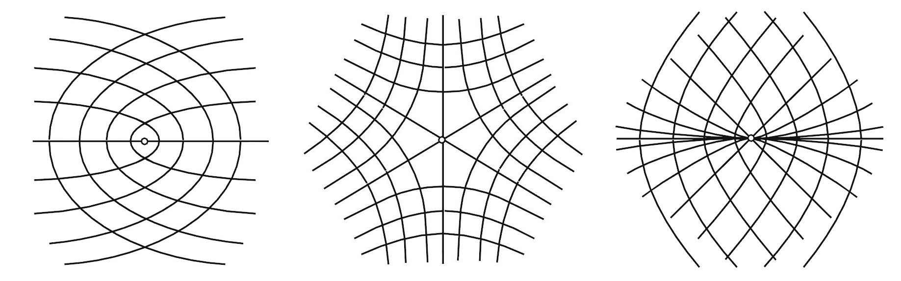
Омбилические точки и сеть линий кривизны поверхности вокруг них. В случае общего положения существуют три топологические различные типа особенности, часто называемые «лимон», «звезда» и «монстар»[1]
Свойства[править]
В точке округления:
- главные кривизны поверхности совпадают.
- Первая квадратичная форма и вторая квадратичная форма поверхности пропорциональны.
- любое касательное направление является главным направлением.
- Соприкасающийся параболоид является параболоидом вращения.
- Индикатриса Дюпена является окружностью.
- Сеть линий кривизны (т.е. линий, касающихся в каждой точке одного из главных направлений поверхности), имеет особенность[1].
- Любая точка округления является либо эллиптической точкой поверхности (если главные кривизны не равны нулю, и следовательно, гауссова кривизна поверхности в данной точке положительная), либо так называемой плоской омбиликой (если главные кривизны равны нулю, и следовательно, гауссова кривизна и средняя кривизна поверхности в данной точке равны нулю). В первом случае в малой окрестности точки округления поверхность похожа на сферу, а во втором — на плоскость.
Примеры[править]
Ошибка создания миниатюры:
Омбилики на трёхосном эллипсоиде
В евклидовом пространстве с метрикой  :
:
- Сфера целиком состоит из эллиптических точек округления.
- Трёхосный эллипсоид (с попарно различными осями) имеет ровно четыре точки округления, все они эллиптическии и относятся к типу «лимон».
- Плоскость целиком состоит из плоских омбилик.
- Обезьянье седло имеет изолированную плоскую омбилику в начале координат.
Гипотеза Каратеодори[править]
Каратеодори высказал гипотезу, что на любой достаточно гладкой замкнутой выпуклой поверхности M в трёхмерном евклидовом пространстве существуют как минимум две омбилические точки. Эта гипотеза была впоследствии доказана при дополнительном предположении, что поверхность M аналитическая[2][3].
Обобщение[править]
Пусть  ― гладкое многообразие произвольной размерности
  в евклидовом пространстве большей размерности. Тогда в каждой точке
  определены
  собственных значений
  пары первой и второй квадратичных форм, заданных на касательном расслоении
  .
.
Точка называется омбиликой, если в ней набор содержит хотя бы два совпадающих числа. Множество омбилик точек имеет коразмерность 2, т.е. задается на двумя независимыми уравнениями.[4] Так, омбилические точки на поверхности общего положения изолированы ( ), а на трёхмерном многообразии общего положения они образуют кривую (
 ).
).
Литература[править]
- Рашевский П.К. Курс дифференциальной геометрии, — Любое издание.
- Фиников С.П. Курс дифференциальной геометрии, — Любое издание.
- Фиников С.П. Теория поверхностей, — Любое издание.
- Porteous I.R. Geometric Differentiation for the intelligence of curves and surfaces — Cambridge University Press, Cambridge, 1994.
- Struik D. J. Lectures on Classical Differential Geometry, — Addison Wesley Publ. Co., 1950. Reprinted by Dover Publ., Inc., 1988.
Примечания[править]
- ↑ 1,0 1,1 Ремизов А.О. Многомерная конструкция Пуанкаре и особенности поднятых полей для неявных дифференциальных уравнений, ― СМФН, 19 (2006), 131–170.
- ↑ Zbl 1056.53003
- ↑ Иванов В. В. Аналитическая гипотеза Каратеодори, ― Сиб. матем. журн., 43:2 (2002), 314–405.
- ↑ Арнольд В.И. Математические методы классической механики, ― Любое издание. (Добавление 10. Кратности собственных частот и эллипсоиды, зависящие от параметров).
Операция округления
постоянно используется в различных
расчетах. При ручных вычислениях обычно
используется симметричное округление.
Правила симметричного округления
изучаются в школе. Существует ещё и
простое отсечение, когда лишние разряды
просто отбрасываются. Такой способ
используется в вычислительной технике.
При округлении
приближенных значений величин получаются
новые приближенные значения, погрешность
которых, как правило, больше погрешности
исходных неокругленных приближенных
значений.
Пусть, например,
известно точное значение величины
![]() =1,234567
=1,234567
и приближенное ее значение![]() =1,234678.
=1,234678.
Округлим![]() ,
,
оставив четыре знака после запятой. В
результате получается новое приближенное
значение![]() =1,2347.
=1,2347.
Абсолютные погрешности![]() и
и![]() равны соответственно:
равны соответственно:![]() =0,000111
=0,000111
и![]() =0,000133.
=0,000133.
Погрешность округленного приближенного
значения величины оказалась больше
погрешности ее неокругленного значения.
Если округлим еще одну цифру, то получим
еще одно приближенное значение![]() =1,235,
=1,235,
погрешность которого будет еще больше![]() =0,000433.
=0,000433.
Чем больше знаковмы
округляем, тем, как правило, больше
абсолютная погрешность.
В некоторых частных
случаях округление может приводить к
уменьшению абсолютной погрешности.
Пусть, например,
![]() =1,234
=1,234
и![]() =1,2342.
=1,2342.
Округлим приближенное значение на одну
цифру и получим округленное приближенное
значение![]() =1,234,
=1,234,
совпадающее с точным. Подобное повышение
точности при округлении возможно, но
возникает редко.
Рассмотрим вопрос
об оценке погрешности округления. Пусть
имеется числовая величина x,
![]()
точное значение,
![]() –
–
некоторое приближенное значение этой
величины, а![]()
результат округления этого приближенного
значения. Назовем величину
![]() погрешностью
погрешностью
округления
и обозначим ее
![]() .
.
Тогда погрешность округленного
приближенного значения
![]() .
.
Следовательно,
![]() .
.
(1.4.1)
Эта формула
позволяет учитывать погрешности
округления.
На практике часто
возникает вопрос о том, как следует
округлять приближенное значение, чтобы
погрешность округленного приближенного
значения была не на многобольше
погрешности неокругленного приближенного
значения величины. Для ответа на этого
вопрос рассмотрим следующий пример.
Пример
1
Пусть точное
значение величины
![]() =1,2345678,
=1,2345678,
а приближенное
![]() =1,2345789.
=1,2345789.
Округлим приближенное
значение четырьмя способами и получим
четыре разных округленных приближенных
значения:
![]() =1,234579,
=1,234579,![]() =1,23458,
=1,23458,![]() =1,2346,
=1,2346,![]() =1,235.
=1,235.
Их погрешности равны соответственно
0,0000112; 0,0000122; 0,0000322; 0,0004322. Погрешность
неокругленного приближенного значения
величины равна 0,0000111. Сравнивая эти
погрешности, можно заметить, что первые
три способа округления не сильно
увеличивают погрешность, а четвертый
способ увеличил погрешность в 40 раз.
Подчеркнем в записи
![]() верные цифры в широком смысле слова:
верные цифры в широком смысле слова:![]() =1,2345789,
=1,2345789,
и сопоставим полученные данные с верными
цифрами в записи неокругленного
приближенного значения. Оказывается,
если при
округлении сохранены все верные цифры,
то погрешность растет не на много,
а если
округляется хотя бы одна верная цифра,
то погрешность вырастает в десятки раз.
Результатом
обобщения многих подобных примеров
является правило, позволяющее округлять
и записывать окончательные результаты
вычислений или измерений. Будем считать,
что известными являются приближенное
значение
![]() и оценка погрешности
и оценка погрешности![]() величиныx.
величиныx.
Соседние файлы в папке ВМ_УЧЕБНИК
- #
- #
- #
- #
- #
- #
- #
- #
- #