In linear algebra, a rotation matrix is a transformation matrix that is used to perform a rotation in Euclidean space. For example, using the convention below, the matrix

rotates points in the xy plane counterclockwise through an angle θ about the origin of a two-dimensional Cartesian coordinate system. To perform the rotation on a plane point with standard coordinates v = (x, y), it should be written as a column vector, and multiplied by the matrix R:

If x and y are the endpoint coordinates of a vector, where x is cosine and y is sine, then the above equations become the trigonometric summation angle formulae. Indeed, a rotation matrix can be seen as the trigonometric summation angle formulae in matrix form. One way to understand this is say we have a vector at an angle 30° from the x axis, and we wish to rotate that angle by a further 45°. We simply need to compute the vector endpoint coordinates at 75°.
The examples in this article apply to active rotations of vectors counterclockwise in a right-handed coordinate system (y counterclockwise from x) by pre-multiplication (R on the left). If any one of these is changed (such as rotating axes instead of vectors, a passive transformation), then the inverse of the example matrix should be used, which coincides with its transpose.
Since matrix multiplication has no effect on the zero vector (the coordinates of the origin), rotation matrices describe rotations about the origin. Rotation matrices provide an algebraic description of such rotations, and are used extensively for computations in geometry, physics, and computer graphics. In some literature, the term rotation is generalized to include improper rotations, characterized by orthogonal matrices with a determinant of −1 (instead of +1). These combine proper rotations with reflections (which invert orientation). In other cases, where reflections are not being considered, the label proper may be dropped. The latter convention is followed in this article.
Rotation matrices are square matrices, with real entries. More specifically, they can be characterized as orthogonal matrices with determinant 1; that is, a square matrix R is a rotation matrix if and only if RT = R−1 and det R = 1. The set of all orthogonal matrices of size n with determinant +1 is a representation of a group known as the special orthogonal group SO(n), one example of which is the rotation group SO(3). The set of all orthogonal matrices of size n with determinant +1 or −1 is a representation of the (general) orthogonal group O(n).
In two dimensions[edit]

A counterclockwise rotation of a vector through angle θ. The vector is initially aligned with the x-axis.
In two dimensions, the standard rotation matrix has the following form:

This rotates column vectors by means of the following matrix multiplication,

Thus, the new coordinates (x′, y′) of a point (x, y) after rotation are

Examples[edit]
For example, when the vector

is rotated by an angle θ, its new coordinates are

and when the vector

is rotated by an angle θ, its new coordinates are

Direction[edit]
The direction of vector rotation is counterclockwise if θ is positive (e.g. 90°), and clockwise if θ is negative (e.g. −90°). Thus the clockwise rotation matrix is found as

The two-dimensional case is the only non-trivial (i.e. not one-dimensional) case where the rotation matrices group is commutative, so that it does not matter in which order multiple rotations are performed. An alternative convention uses rotating axes,[1] and the above matrices also represent a rotation of the axes clockwise through an angle θ.
Non-standard orientation of the coordinate system[edit]

A rotation through angle θ with non-standard axes.
If a standard right-handed Cartesian coordinate system is used, with the x-axis to the right and the y-axis up, the rotation R(θ) is counterclockwise. If a left-handed Cartesian coordinate system is used, with x directed to the right but y directed down, R(θ) is clockwise. Such non-standard orientations are rarely used in mathematics but are common in 2D computer graphics, which often have the origin in the top left corner and the y-axis down the screen or page.[2]
See below for other alternative conventions which may change the sense of the rotation produced by a rotation matrix.
Common rotations[edit]
Particularly useful are the matrices
![{displaystyle {begin{bmatrix}0&-1\[3pt]1&0\end{bmatrix}},quad {begin{bmatrix}-1&0\[3pt]0&-1\end{bmatrix}},quad {begin{bmatrix}0&1\[3pt]-1&0\end{bmatrix}}}](https://wikimedia.org/api/rest_v1/media/math/render/svg/049475f6bbfd9cfe4f0db0e7f063301e7acb774b)
for 90°, 180°, and 270° counter-clockwise rotations.
A 180° rotation (middle) followed by a positive 90° rotation (left) is equivalent to a single negative 90° (positive 270°) rotation (right). Each of these figures depicts the result of a rotation relative to an upright starting position (bottom left) and includes the matrix representation of the permutation applied by the rotation (center right), as well as other related diagrams. See «Permutation notation» on Wikiversity for details.
Relationship with complex plane[edit]
Since

the matrices of the shape

form a ring isomorphic to the field of the complex numbers  . Under this isomorphism, the rotation matrices correspond to circle of the unit complex numbers, the complex numbers of modulus 1.
If one identifies  with through the linear isomorphism
  the action of a matrix of the above form on vectors of corresponds to the multiplication by the complex number x + iy, and rotations correspond to multiplication by complex numbers of modulus 1.
As every rotation matrix can be written

the above correspondence associates such a matrix with the complex number

(this last equality is Euler’s formula).
In three dimensions[edit]
A positive 90° rotation around the y-axis (left) after one around the z-axis (middle) gives a 120° rotation around the main diagonal (right).
In the top left corner are the rotation matrices, in the bottom right corner are the corresponding permutations of the cube with the origin in its center.
Basic rotations[edit]
A basic rotation (also called elemental rotation) is a rotation about one of the axes of a coordinate system. The following three basic rotation matrices rotate vectors by an angle θ about the x-, y-, or z-axis, in three dimensions, using the right-hand rule—which codifies their alternating signs. Notice that the right-hand rule only works when multiplying  . (The same matrices can also represent a clockwise rotation of the axes.[nb 1])
![{displaystyle {begin{alignedat}{1}R_{x}(theta )&={begin{bmatrix}1&0&0\0&cos theta &-sin theta \[3pt]0&sin theta &cos theta \[3pt]end{bmatrix}}\[6pt]R_{y}(theta )&={begin{bmatrix}cos theta &0&sin theta \[3pt]0&1&0\[3pt]-sin theta &0&cos theta \end{bmatrix}}\[6pt]R_{z}(theta )&={begin{bmatrix}cos theta &-sin theta &0\[3pt]sin theta &cos theta &0\[3pt]0&0&1\end{bmatrix}}end{alignedat}}}](https://wikimedia.org/api/rest_v1/media/math/render/svg/a6821937d5031de282a190f75312353c970aa2df)
For column vectors, each of these basic vector rotations appears counterclockwise when the axis about which they occur points toward the observer, the coordinate system is right-handed, and the angle θ is positive. Rz, for instance, would rotate toward the y-axis a vector aligned with the x-axis, as can easily be checked by operating with Rz on the vector (1,0,0):

This is similar to the rotation produced by the above-mentioned two-dimensional rotation matrix. See below for alternative conventions which may apparently or actually invert the sense of the rotation produced by these matrices.
General rotations[edit]
Other rotation matrices can be obtained from these three using matrix multiplication. For example, the product

represents a rotation whose yaw, pitch, and roll angles are α, β and γ, respectively. More formally, it is an intrinsic rotation whose Tait–Bryan angles are α, β, γ, about axes z, y, x, respectively.
Similarly, the product

represents an extrinsic rotation whose (improper) Euler angles are α, β, γ, about axes x, y, z.
These matrices produce the desired effect only if they are used to premultiply column vectors, and (since in general matrix multiplication is not commutative) only if they are applied in the specified order (see Ambiguities for more details). The order of rotation operations is from right to left; the matrix adjacent to the column vector is the first to be applied, and then the one to the left.[3]
Conversion from rotation matrix to axis–angle[edit]
Every rotation in three dimensions is defined by its axis (a vector along this axis is unchanged by the rotation), and its angle — the amount of rotation about that axis (Euler rotation theorem).
There are several methods to compute the axis and angle from a rotation matrix (see also axis–angle representation). Here, we only describe the method based on the computation of the eigenvectors and eigenvalues of the rotation matrix. It is also possible to use the trace of the rotation matrix.
Determining the axis[edit]
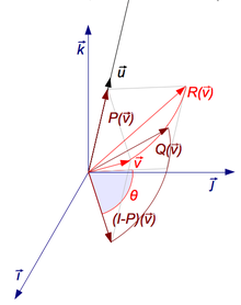
A rotation R around axis u can be decomposed using 3 endomorphisms P, (I − P), and Q (click to enlarge).
Given a 3 × 3 rotation matrix R, a vector u parallel to the rotation axis must satisfy

since the rotation of u around the rotation axis must result in u. The equation above may be solved for u which is unique up to a scalar factor unless R = I.
Further, the equation may be rewritten

which shows that u lies in the null space of R − I.
Viewed in another way, u is an eigenvector of R corresponding to the eigenvalue λ = 1. Every rotation matrix must have this eigenvalue, the other two eigenvalues being complex conjugates of each other. It follows that a general rotation matrix in three dimensions has, up to a multiplicative constant, only one real eigenvector.
One way to determine the rotation axis is by showing that:

Since (R − RT) is a skew-symmetric matrix, we can choose u such that
![{displaystyle [mathbf {u} ]_{times }=left(R-R^{mathsf {T}}right).}](https://wikimedia.org/api/rest_v1/media/math/render/svg/4f918d62cae11c81d33160177d9583d6e7efbe2d)
The matrix–vector product becomes a cross product of a vector with itself, ensuring that the result is zero:
![{displaystyle left(R-R^{mathsf {T}}right)mathbf {u} =[mathbf {u} ]_{times }mathbf {u} =mathbf {u} times mathbf {u} =0,}](https://wikimedia.org/api/rest_v1/media/math/render/svg/11848fee25bc229562a029195d181540a87e8597)
Therefore, if

then

The magnitude of u computed this way is ‖u‖ = 2 sin θ, where θ is the angle of rotation.
This does not work if R is symmetric. Above, if R − RT is zero, then all subsequent steps are invalid. In this case, it is necessary to diagonalize R and find the eigenvector corresponding to an eigenvalue of 1.
Determining the angle[edit]
To find the angle of a rotation, once the axis of the rotation is known, select a vector v perpendicular to the axis. Then the angle of the rotation is the angle between v and Rv.
A more direct method, however, is to simply calculate the trace: the sum of the diagonal elements of the rotation matrix. Care should be taken to select the right sign for the angle θ to match the chosen axis:

from which follows that the angle’s absolute value is

Rotation matrix from axis and angle[edit]
The matrix of a proper rotation R by angle θ around the axis u = (ux, uy, uz), a unit vector with u2
x + u2
y + u2
z = 1, is given by:[4]

A derivation of this matrix from first principles can be found in section 9.2 here.[5] The basic idea to derive this matrix is dividing the problem into few known simple steps.
- First rotate the given axis and the point such that the axis lies in one of the coordinate planes (xy, yz or zx)
- Then rotate the given axis and the point such that the axis is aligned with one of the two coordinate axes for that particular coordinate plane (x, y or z)
- Use one of the fundamental rotation matrices to rotate the point depending on the coordinate axis with which the rotation axis is aligned.
- Reverse rotate the axis-point pair such that it attains the final configuration as that was in step 2 (Undoing step 2)
- Reverse rotate the axis-point pair which was done in step 1 (undoing step 1)
This can be written more concisely as
![{displaystyle R=(cos theta ),I+(sin theta ),[mathbf {u} ]_{times }+(1-cos theta ),(mathbf {u} otimes mathbf {u} ),}](https://wikimedia.org/api/rest_v1/media/math/render/svg/5865faae48e2c8bca9a0780d52fec23a768e5354)
where [u]× is the cross product matrix of u; the expression u ⊗ u is the outer product, and I is the identity matrix. Alternatively, the matrix entries are:

where εjkl is the Levi-Civita symbol with ε123 = 1. This is a matrix form of Rodrigues’ rotation formula, (or the equivalent, differently parametrized Euler–Rodrigues formula) with[nb 2]
![{displaystyle mathbf {u} otimes mathbf {u} =mathbf {u} mathbf {u} ^{mathsf {T}}={begin{bmatrix}u_{x}^{2}&u_{x}u_{y}&u_{x}u_{z}\[3pt]u_{x}u_{y}&u_{y}^{2}&u_{y}u_{z}\[3pt]u_{x}u_{z}&u_{y}u_{z}&u_{z}^{2}end{bmatrix}},qquad [mathbf {u} ]_{times }={begin{bmatrix}0&-u_{z}&u_{y}\[3pt]u_{z}&0&-u_{x}\[3pt]-u_{y}&u_{x}&0end{bmatrix}}.}](https://wikimedia.org/api/rest_v1/media/math/render/svg/e3ddca93f49b042e6a14d5263002603fc0738308)
In  the rotation of a vector x around the axis u by an angle θ can be written as:

If the 3D space is right-handed and θ > 0, this rotation will be counterclockwise when u points towards the observer (Right-hand rule). Explicitly, with  a right-handed orthonormal basis,

Note the striking merely apparent differences to the equivalent Lie-algebraic formulation below.
Properties[edit]
For any n-dimensional rotation matrix R acting on 
 (The rotation is an orthogonal matrix)

It follows that:

A rotation is termed proper if det R = 1, and improper (or a roto-reflection) if det R = –1. For even dimensions n = 2k, the n eigenvalues λ of a proper rotation occur as pairs of complex conjugates which are roots of unity: λ = e±iθj for j = 1, …, k, which is real only for λ = ±1. Therefore, there may be no vectors fixed by the rotation (λ = 1), and thus no axis of rotation. Any fixed eigenvectors occur in pairs, and the axis of rotation is an even-dimensional subspace.
For odd dimensions n = 2k + 1, a proper rotation R will have an odd number of eigenvalues, with at least one λ = 1 and the axis of rotation will be an odd dimensional subspace. Proof:

Here I is the identity matrix, and we use det(RT) = det(R) = 1, as well as (−1)n = −1 since n is odd. Therefore, det(R – I) = 0, meaning there is a null vector v with (R – I)v = 0, that is Rv = v, a fixed eigenvector. There may also be pairs of fixed eigenvectors in the even-dimensional subspace orthogonal to v, so the total dimension of fixed eigenvectors is odd.
For example, in 2-space n = 2, a rotation by angle θ has eigenvalues λ = eiθ and λ = e−iθ, so there is no axis of rotation except when θ = 0, the case of the null rotation. In 3-space n = 3, the axis of a non-null proper rotation is always a unique line, and a rotation around this axis by angle θ has eigenvalues λ = 1, eiθ, e−iθ. In 4-space n = 4, the four eigenvalues are of the form e±iθ, e±iφ. The null rotation has θ = φ = 0. The case of θ = 0, φ ≠ 0 is called a simple rotation, with two unit eigenvalues forming an axis plane, and a two-dimensional rotation orthogonal to the axis plane. Otherwise, there is no axis plane. The case of θ = φ is called an isoclinic rotation, having eigenvalues e±iθ repeated twice, so every vector is rotated through an angle θ.
The trace of a rotation matrix is equal to the sum of its eigenvalues. For n = 2, a rotation by angle θ has trace 2 cos θ. For n = 3, a rotation around any axis by angle θ has trace 1 + 2 cos θ. For n = 4, and the trace is 2(cos θ + cos φ), which becomes 4 cos θ for an isoclinic rotation.
Examples[edit]
|
|


Geometry[edit]
In Euclidean geometry, a rotation is an example of an isometry, a transformation that moves points without changing the distances between them. Rotations are distinguished from other isometries by two additional properties: they leave (at least) one point fixed, and they leave «handedness» unchanged. In contrast, a translation moves every point, a reflection exchanges left- and right-handed ordering, a glide reflection does both, and an improper rotation combines a change in handedness with a normal rotation.
If a fixed point is taken as the origin of a Cartesian coordinate system, then every point can be given coordinates as a displacement from the origin. Thus one may work with the vector space of displacements instead of the points themselves. Now suppose (p1, …, pn) are the coordinates of the vector p from the origin O to point P. Choose an orthonormal basis for our coordinates; then the squared distance to P, by Pythagoras, is

which can be computed using the matrix multiplication

A geometric rotation transforms lines to lines, and preserves ratios of distances between points. From these properties it can be shown that a rotation is a linear transformation of the vectors, and thus can be written in matrix form, Qp. The fact that a rotation preserves, not just ratios, but distances themselves, is stated as

or

Because this equation holds for all vectors, p, one concludes that every rotation matrix, Q, satisfies the orthogonality condition,

Rotations preserve handedness because they cannot change the ordering of the axes, which implies the special matrix condition,

Equally important, it can be shown that any matrix satisfying these two conditions acts as a rotation.
Multiplication[edit]
The inverse of a rotation matrix is its transpose, which is also a rotation matrix:

The product of two rotation matrices is a rotation matrix:

For n > 2, multiplication of n × n rotation matrices is generally not commutative.

Noting that any identity matrix is a rotation matrix, and that matrix multiplication is associative, we may summarize all these properties by saying that the n × n rotation matrices form a group, which for n > 2 is non-abelian, called a special orthogonal group, and denoted by SO(n), SO(n,R), SOn, or SOn(R), the group of n × n rotation matrices is isomorphic to the group of rotations in an n-dimensional space. This means that multiplication of rotation matrices corresponds to composition of rotations, applied in left-to-right order of their corresponding matrices.
Ambiguities[edit]

Alias and alibi rotations
The interpretation of a rotation matrix can be subject to many ambiguities.
In most cases the effect of the ambiguity is equivalent to the effect of a rotation matrix inversion (for these orthogonal matrices equivalently matrix transpose).
- Alias or alibi (passive or active) transformation
- The coordinates of a point P may change due to either a rotation of the coordinate system CS (alias), or a rotation of the point P (alibi). In the latter case, the rotation of P also produces a rotation of the vector v representing P. In other words, either P and v are fixed while CS rotates (alias), or CS is fixed while P and v rotate (alibi). Any given rotation can be legitimately described both ways, as vectors and coordinate systems actually rotate with respect to each other, about the same axis but in opposite directions. Throughout this article, we chose the alibi approach to describe rotations. For instance,
- represents a counterclockwise rotation of a vector v by an angle θ, or a rotation of CS by the same angle but in the opposite direction (i.e. clockwise). Alibi and alias transformations are also known as active and passive transformations, respectively.
- Pre-multiplication or post-multiplication
- The same point P can be represented either by a column vector v or a row vector w. Rotation matrices can either pre-multiply column vectors (Rv), or post-multiply row vectors (wR). However, Rv produces a rotation in the opposite direction with respect to wR. Throughout this article, rotations produced on column vectors are described by means of a pre-multiplication. To obtain exactly the same rotation (i.e. the same final coordinates of point P), the equivalent row vector must be post-multiplied by the transpose of R (i.e. wRT).
- Right- or left-handed coordinates
- The matrix and the vector can be represented with respect to a right-handed or left-handed coordinate system. Throughout the article, we assumed a right-handed orientation, unless otherwise specified.
- Vectors or forms
- The vector space has a dual space of linear forms, and the matrix can act on either vectors or forms.

Decompositions[edit]
Independent planes[edit]
Consider the 3 × 3 rotation matrix

If Q acts in a certain direction, v, purely as a scaling by a factor λ, then we have

so that

Thus λ is a root of the characteristic polynomial for Q,

Two features are noteworthy. First, one of the roots (or eigenvalues) is 1, which tells us that some direction is unaffected by the matrix. For rotations in three dimensions, this is the axis of the rotation (a concept that has no meaning in any other dimension). Second, the other two roots are a pair of complex conjugates, whose product is 1 (the constant term of the quadratic), and whose sum is 2 cos θ (the negated linear term). This factorization is of interest for 3 × 3 rotation matrices because the same thing occurs for all of them. (As special cases, for a null rotation the «complex conjugates» are both 1, and for a 180° rotation they are both −1.) Furthermore, a similar factorization holds for any n × n rotation matrix. If the dimension, n, is odd, there will be a «dangling» eigenvalue of 1; and for any dimension the rest of the polynomial factors into quadratic terms like the one here (with the two special cases noted). We are guaranteed that the characteristic polynomial will have degree n and thus n eigenvalues. And since a rotation matrix commutes with its transpose, it is a normal matrix, so can be diagonalized. We conclude that every rotation matrix, when expressed in a suitable coordinate system, partitions into independent rotations of two-dimensional subspaces, at most n/2 of them.
The sum of the entries on the main diagonal of a matrix is called the trace; it does not change if we reorient the coordinate system, and always equals the sum of the eigenvalues. This has the convenient implication for 2 × 2 and 3 × 3 rotation matrices that the trace reveals the angle of rotation, θ, in the two-dimensional space (or subspace). For a 2 × 2 matrix the trace is 2 cos θ, and for a 3 × 3 matrix it is 1 + 2 cos θ. In the three-dimensional case, the subspace consists of all vectors perpendicular to the rotation axis (the invariant direction, with eigenvalue 1). Thus we can extract from any 3 × 3 rotation matrix a rotation axis and an angle, and these completely determine the rotation.
Sequential angles[edit]
The constraints on a 2 × 2 rotation matrix imply that it must have the form

with a2 + b2 = 1. Therefore, we may set a = cos θ and b = sin θ, for some angle θ. To solve for θ it is not enough to look at a alone or b alone; we must consider both together to place the angle in the correct quadrant, using a two-argument arctangent function.
Now consider the first column of a 3 × 3 rotation matrix,

Although a2 + b2 will probably not equal 1, but some value r2 < 1, we can use a slight variation of the previous computation to find a so-called Givens rotation that transforms the column to

zeroing b. This acts on the subspace spanned by the x— and y-axes. We can then repeat the process for the xz-subspace to zero c. Acting on the full matrix, these two rotations produce the schematic form

Shifting attention to the second column, a Givens rotation of the yz-subspace can now zero the z value. This brings the full matrix to the form

which is an identity matrix. Thus we have decomposed Q as

An n × n rotation matrix will have (n − 1) + (n − 2) + ⋯ + 2 + 1, or

entries below the diagonal to zero. We can zero them by extending the same idea of stepping through the columns with a series of rotations in a fixed sequence of planes. We conclude that the set of n × n rotation matrices, each of which has n2 entries, can be parameterized by 1/2n(n − 1) angles.
| xzxw | xzyw | xyxw | xyzw |
| yxyw | yxzw | yzyw | yzxw |
| zyzw | zyxw | zxzw | zxyw |
| xzxb | yzxb | xyxb | zyxb |
| yxyb | zxyb | yzyb | xzyb |
| zyzb | xyzb | zxzb | yxzb |
In three dimensions this restates in matrix form an observation made by Euler, so mathematicians call the ordered sequence of three angles Euler angles. However, the situation is somewhat more complicated than we have so far indicated. Despite the small dimension, we actually have considerable freedom in the sequence of axis pairs we use; and we also have some freedom in the choice of angles. Thus we find many different conventions employed when three-dimensional rotations are parameterized for physics, or medicine, or chemistry, or other disciplines. When we include the option of world axes or body axes, 24 different sequences are possible. And while some disciplines call any sequence Euler angles, others give different names (Cardano, Tait–Bryan, roll-pitch-yaw) to different sequences.
One reason for the large number of options is that, as noted previously, rotations in three dimensions (and higher) do not commute. If we reverse a given sequence of rotations, we get a different outcome. This also implies that we cannot compose two rotations by adding their corresponding angles. Thus Euler angles are not vectors, despite a similarity in appearance as a triplet of numbers.
Nested dimensions[edit]
A 3 × 3 rotation matrix such as

suggests a 2 × 2 rotation matrix,

is embedded in the upper left corner:
![{displaystyle Q_{3times 3}=left[{begin{matrix}Q_{2times 2}&mathbf {0} \mathbf {0} ^{mathsf {T}}&1end{matrix}}right].}](https://wikimedia.org/api/rest_v1/media/math/render/svg/6f439ce8b73f47040b70c9b64ab7fa89d91c46a6)
This is no illusion; not just one, but many, copies of n-dimensional rotations are found within (n + 1)-dimensional rotations, as subgroups. Each embedding leaves one direction fixed, which in the case of 3 × 3 matrices is the rotation axis. For example, we have
![{displaystyle {begin{aligned}Q_{mathbf {x} }(theta )&={begin{bmatrix}{color {CadetBlue}1}&{color {CadetBlue}0}&{color {CadetBlue}0}\{color {CadetBlue}0}&cos theta &-sin theta \{color {CadetBlue}0}&sin theta &cos theta end{bmatrix}},\[8px]Q_{mathbf {y} }(theta )&={begin{bmatrix}cos theta &{color {CadetBlue}0}&sin theta \{color {CadetBlue}0}&{color {CadetBlue}1}&{color {CadetBlue}0}\-sin theta &{color {CadetBlue}0}&cos theta end{bmatrix}},\[8px]Q_{mathbf {z} }(theta )&={begin{bmatrix}cos theta &-sin theta &{color {CadetBlue}0}\sin theta &cos theta &{color {CadetBlue}0}\{color {CadetBlue}0}&{color {CadetBlue}0}&{color {CadetBlue}1}end{bmatrix}},end{aligned}}}](https://wikimedia.org/api/rest_v1/media/math/render/svg/63ce9d4e595deed5ef5572d36ec99821e1b021e2)
fixing the x-axis, the y-axis, and the z-axis, respectively. The rotation axis need not be a coordinate axis; if u = (x,y,z) is a unit vector in the desired direction, then
![{displaystyle {begin{aligned}Q_{mathbf {u} }(theta )&={begin{bmatrix}0&-z&y\z&0&-x\-y&x&0end{bmatrix}}sin theta +left(I-mathbf {u} mathbf {u} ^{mathsf {T}}right)cos theta +mathbf {u} mathbf {u} ^{mathsf {T}}\[8px]&={begin{bmatrix}left(1-x^{2}right)c_{theta }+x^{2}&-zs_{theta }-xyc_{theta }+xy&ys_{theta }-xzc_{theta }+xz\zs_{theta }-xyc_{theta }+xy&left(1-y^{2}right)c_{theta }+y^{2}&-xs_{theta }-yzc_{theta }+yz\-ys_{theta }-xzc_{theta }+xz&xs_{theta }-yzc_{theta }+yz&left(1-z^{2}right)c_{theta }+z^{2}end{bmatrix}}\[8px]&={begin{bmatrix}x^{2}(1-c_{theta })+c_{theta }&xy(1-c_{theta })-zs_{theta }&xz(1-c_{theta })+ys_{theta }\xy(1-c_{theta })+zs_{theta }&y^{2}(1-c_{theta })+c_{theta }&yz(1-c_{theta })-xs_{theta }\xz(1-c_{theta })-ys_{theta }&yz(1-c_{theta })+xs_{theta }&z^{2}(1-c_{theta })+c_{theta }end{bmatrix}},end{aligned}}}](https://wikimedia.org/api/rest_v1/media/math/render/svg/87042389f5f93fc21a43beafc126d3ea5a9ee177)
where cθ = cos θ, sθ = sin θ, is a rotation by angle θ leaving axis u fixed.
A direction in (n + 1)-dimensional space will be a unit magnitude vector, which we may consider a point on a generalized sphere, Sn. Thus it is natural to describe the rotation group SO(n + 1) as combining SO(n) and Sn. A suitable formalism is the fiber bundle,

where for every direction in the base space, Sn, the fiber over it in the total space, SO(n + 1), is a copy of the fiber space, SO(n), namely the rotations that keep that direction fixed.
Thus we can build an n × n rotation matrix by starting with a 2 × 2 matrix, aiming its fixed axis on S2 (the ordinary sphere in three-dimensional space), aiming the resulting rotation on S3, and so on up through Sn−1. A point on Sn can be selected using n numbers, so we again have 1/2n(n − 1) numbers to describe any n × n rotation matrix.
In fact, we can view the sequential angle decomposition, discussed previously, as reversing this process. The composition of n − 1 Givens rotations brings the first column (and row) to (1, 0, …, 0), so that the remainder of the matrix is a rotation matrix of dimension one less, embedded so as to leave (1, 0, …, 0) fixed.
Skew parameters via Cayley’s formula[edit]
When an n × n rotation matrix Q, does not include a −1 eigenvalue, thus none of the planar rotations which it comprises are 180° rotations, then Q + I is an invertible matrix. Most rotation matrices fit this description, and for them it can be shown that (Q − I)(Q + I)−1 is a skew-symmetric matrix, A. Thus AT = −A; and since the diagonal is necessarily zero, and since the upper triangle determines the lower one, A contains 1/2n(n − 1) independent numbers.
Conveniently, I − A is invertible whenever A is skew-symmetric; thus we can recover the original matrix using the Cayley transform,

which maps any skew-symmetric matrix A to a rotation matrix. In fact, aside from the noted exceptions, we can produce any rotation matrix in this way. Although in practical applications we can hardly afford to ignore 180° rotations, the Cayley transform is still a potentially useful tool, giving a parameterization of most rotation matrices without trigonometric functions.
In three dimensions, for example, we have (Cayley 1846)
![{displaystyle {begin{aligned}&{begin{bmatrix}0&-z&y\z&0&-x\-y&x&0end{bmatrix}}mapsto \[3pt]quad {frac {1}{1+x^{2}+y^{2}+z^{2}}}&{begin{bmatrix}1+x^{2}-y^{2}-z^{2}&2xy-2z&2y+2xz\2xy+2z&1-x^{2}+y^{2}-z^{2}&2yz-2x\2xz-2y&2x+2yz&1-x^{2}-y^{2}+z^{2}end{bmatrix}}.end{aligned}}}](https://wikimedia.org/api/rest_v1/media/math/render/svg/ad82b169b68ec60349be493378761aab543c9cf8)
If we condense the skew entries into a vector, (x,y,z), then we produce a 90° rotation around the x-axis for (1, 0, 0), around the y-axis for (0, 1, 0), and around the z-axis for (0, 0, 1). The 180° rotations are just out of reach; for, in the limit as x → ∞, (x, 0, 0) does approach a 180° rotation around the x axis, and similarly for other directions.
Decomposition into shears[edit]
For the 2D case, a rotation matrix can be decomposed into three shear matrices (Paeth 1986):

This is useful, for instance, in computer graphics, since shears can be implemented with fewer multiplication instructions than rotating a bitmap directly. On modern computers, this may not matter, but it can be relevant for very old or low-end microprocessors.
A rotation can also be written as two shears and scaling (Daubechies & Sweldens 1998):

Group theory[edit]
Below follow some basic facts about the role of the collection of all rotation matrices of a fixed dimension (here mostly 3) in mathematics and particularly in physics where rotational symmetry is a requirement of every truly fundamental law (due to the assumption of isotropy of space), and where the same symmetry, when present, is a simplifying property of many problems of less fundamental nature. Examples abound in classical mechanics and quantum mechanics. Knowledge of the part of the solutions pertaining to this symmetry applies (with qualifications) to all such problems and it can be factored out of a specific problem at hand, thus reducing its complexity. A prime example – in mathematics and physics – would be the theory of spherical harmonics. Their role in the group theory of the rotation groups is that of being a representation space for the entire set of finite-dimensional irreducible representations of the rotation group SO(3). For this topic, see Rotation group SO(3) § Spherical harmonics.
The main articles listed in each subsection are referred to for more detail.
Lie group[edit]
The n × n rotation matrices for each n form a group, the special orthogonal group, SO(n). This algebraic structure is coupled with a topological structure inherited from  in such a way that the operations of multiplication and taking the inverse are analytic functions of the matrix entries. Thus SO(n) is for each n a Lie group. It is compact and connected, but not simply connected. It is also a semi-simple group, in fact a simple group with the exception SO(4).[6] The relevance of this is that all theorems and all machinery from the theory of analytic manifolds (analytic manifolds are in particular smooth manifolds) apply and the well-developed representation theory of compact semi-simple groups is ready for use.
Lie algebra[edit]
The Lie algebra so(n) of SO(n) is given by

and is the space of skew-symmetric matrices of dimension n, see classical group, where o(n) is the Lie algebra of O(n), the orthogonal group. For reference, the most common basis for so(3) is

Exponential map[edit]
Connecting the Lie algebra to the Lie group is the exponential map, which is defined using the standard matrix exponential series for eA[7] For any skew-symmetric matrix A, exp(A) is always a rotation matrix.[nb 3]
An important practical example is the 3 × 3 case. In rotation group SO(3), it is shown that one can identify every A ∈ so(3) with an Euler vector ω = θu, where u = (x, y, z) is a unit magnitude vector.
By the properties of the identification  , u is in the null space of A. Thus, u is left invariant by exp(A) and is hence a rotation axis.
According to Rodrigues’ rotation formula on matrix form, one obtains,

where

This is the matrix for a rotation around axis u by the angle θ. For full detail, see exponential map SO(3).
Baker–Campbell–Hausdorff formula[edit]
The BCH formula provides an explicit expression for Z = log(eXeY) in terms of a series expansion of nested commutators of X and Y.[8] This general expansion unfolds as[nb 4]
![{displaystyle Z=C(X,Y)=X+Y+{tfrac {1}{2}}[X,Y]+{tfrac {1}{12}}{bigl [}X,[X,Y]{bigr ]}-{tfrac {1}{12}}{bigl [}Y,[X,Y]{bigr ]}+cdots .}](https://wikimedia.org/api/rest_v1/media/math/render/svg/18d3139eecb4a3799df3f187e78c1b3f0cb2f3bf)
In the 3 × 3 case, the general infinite expansion has a compact form,[9]
![Z=alpha X+beta Y+gamma [X,Y],](https://wikimedia.org/api/rest_v1/media/math/render/svg/1cdd2c4da063f9ec30359beaacd3767b962f3875)
for suitable trigonometric function coefficients, detailed in the Baker–Campbell–Hausdorff formula for SO(3).
As a group identity, the above holds for all faithful representations, including the doublet (spinor representation), which is simpler. The same explicit formula thus follows straightforwardly through Pauli matrices; see the 2 × 2 derivation for SU(2). For the general n × n case, one might use Ref.[10]
Spin group[edit]
The Lie group of n × n rotation matrices, SO(n), is not simply connected, so Lie theory tells us it is a homomorphic image of a universal covering group. Often the covering group, which in this case is called the spin group denoted by Spin(n), is simpler and more natural to work with.[11]
In the case of planar rotations, SO(2) is topologically a circle, S1. Its universal covering group, Spin(2), is isomorphic to the real line, R, under addition. Whenever angles of arbitrary magnitude are used one is taking advantage of the convenience of the universal cover. Every 2 × 2 rotation matrix is produced by a countable infinity of angles, separated by integer multiples of 2π. Correspondingly, the fundamental group of SO(2) is isomorphic to the integers, Z.
In the case of spatial rotations, SO(3) is topologically equivalent to three-dimensional real projective space, RP3. Its universal covering group, Spin(3), is isomorphic to the 3-sphere, S3. Every 3 × 3 rotation matrix is produced by two opposite points on the sphere. Correspondingly, the fundamental group of SO(3) is isomorphic to the two-element group, Z2.
We can also describe Spin(3) as isomorphic to quaternions of unit norm under multiplication, or to certain 4 × 4 real matrices, or to 2 × 2 complex special unitary matrices, namely SU(2). The covering maps for the first and the last case are given by

and

For a detailed account of the SU(2)-covering and the quaternionic covering, see spin group SO(3).
Many features of these cases are the same for higher dimensions. The coverings are all two-to-one, with SO(n), n > 2, having fundamental group Z2. The natural setting for these groups is within a Clifford algebra. One type of action of the rotations is produced by a kind of «sandwich», denoted by qvq∗. More importantly in applications to physics, the corresponding spin representation of the Lie algebra sits inside the Clifford algebra. It can be exponentiated in the usual way to give rise to a 2-valued representation, also known as projective representation of the rotation group. This is the case with SO(3) and SU(2), where the 2-valued representation can be viewed as an «inverse» of the covering map. By properties of covering maps, the inverse can be chosen ono-to-one as a local section, but not globally.
Infinitesimal rotations[edit]
The matrices in the Lie algebra are not themselves rotations; the skew-symmetric matrices are derivatives, proportional differences of rotations. An actual «differential rotation», or infinitesimal rotation matrix has the form

where dθ is vanishingly small and A ∈ so(n), for instance with A = Lx,

The computation rules are as usual except that infinitesimals of second order are routinely dropped. With these rules, these matrices do not satisfy all the same properties as ordinary finite rotation matrices under the usual treatment of infinitesimals.[12] It turns out that the order in which infinitesimal rotations are applied is irrelevant. To see this exemplified, consult infinitesimal rotations SO(3).
Conversions[edit]
We have seen the existence of several decompositions that apply in any dimension, namely independent planes, sequential angles, and nested dimensions. In all these cases we can either decompose a matrix or construct one. We have also given special attention to 3 × 3 rotation matrices, and these warrant further attention, in both directions (Stuelpnagel 1964).
Quaternion[edit]
Given the unit quaternion q = w + xi + yj + zk, the equivalent pre-multiplied (to be used with column vectors) 3 × 3 rotation matrix is [13]

Now every quaternion component appears multiplied by two in a term of degree two, and if all such terms are zero what is left is an identity matrix. This leads to an efficient, robust conversion from any quaternion – whether unit or non-unit – to a 3 × 3 rotation matrix. Given:

we can calculate

Freed from the demand for a unit quaternion, we find that nonzero quaternions act as homogeneous coordinates for 3 × 3 rotation matrices. The Cayley transform, discussed earlier, is obtained by scaling the quaternion so that its w component is 1. For a 180° rotation around any axis, w will be zero, which explains the Cayley limitation.
The sum of the entries along the main diagonal (the trace), plus one, equals 4 − 4(x2 + y2 + z2), which is 4w2. Thus we can write the trace itself as 2w2 + 2w2 − 1; and from the previous version of the matrix we see that the diagonal entries themselves have the same form: 2x2 + 2w2 − 1, 2y2 + 2w2 − 1, and 2z2 + 2w2 − 1. So we can easily compare the magnitudes of all four quaternion components using the matrix diagonal. We can, in fact, obtain all four magnitudes using sums and square roots, and choose consistent signs using the skew-symmetric part of the off-diagonal entries:

Alternatively, use a single square root and division

This is numerically stable so long as the trace, t, is not negative; otherwise, we risk dividing by (nearly) zero. In that case, suppose Qxx is the largest diagonal entry, so x will have the largest magnitude (the other cases are derived by cyclic permutation); then the following is safe.

If the matrix contains significant error, such as accumulated numerical error, we may construct a symmetric 4 × 4 matrix,

and find the eigenvector, (x, y, z, w), of its largest magnitude eigenvalue. (If Q is truly a rotation matrix, that value will be 1.) The quaternion so obtained will correspond to the rotation matrix closest to the given matrix (Bar-Itzhack 2000) (Note: formulation of the cited article is post-multiplied, works with row vectors).
Polar decomposition[edit]
If the n × n matrix M is nonsingular, its columns are linearly independent vectors; thus the Gram–Schmidt process can adjust them to be an orthonormal basis. Stated in terms of numerical linear algebra, we convert M to an orthogonal matrix, Q, using QR decomposition. However, we often prefer a Q closest to M, which this method does not accomplish. For that, the tool we want is the polar decomposition (Fan & Hoffman 1955; Higham 1989).
To measure closeness, we may use any matrix norm invariant under orthogonal transformations. A convenient choice is the Frobenius norm, ‖Q − M‖F, squared, which is the sum of the squares of the element differences. Writing this in terms of the trace, Tr, our goal is,
- Find Q minimizing Tr( (Q − M)T(Q − M) ), subject to QTQ = I.
Though written in matrix terms, the objective function is just a quadratic polynomial. We can minimize it in the usual way, by finding where its derivative is zero. For a 3 × 3 matrix, the orthogonality constraint implies six scalar equalities that the entries of Q must satisfy. To incorporate the constraint(s), we may employ a standard technique, Lagrange multipliers, assembled as a symmetric matrix, Y. Thus our method is:
- Differentiate Tr( (Q − M)T(Q − M) + (QTQ − I)Y ) with respect to (the entries of) Q, and equate to zero.
Consider a 2 × 2 example. Including constraints, we seek to minimize

Taking the derivative with respect to Qxx, Qxy, Qyx, Qyy in turn, we assemble a matrix.

In general, we obtain the equation

so that

where Q is orthogonal and S is symmetric. To ensure a minimum, the Y matrix (and hence S) must be positive definite. Linear algebra calls QS the polar decomposition of M, with S the positive square root of S2 = MTM.

When M is non-singular, the Q and S factors of the polar decomposition are uniquely determined. However, the determinant of S is positive because S is positive definite, so Q inherits the sign of the determinant of M. That is, Q is only guaranteed to be orthogonal, not a rotation matrix. This is unavoidable; an M with negative determinant has no uniquely defined closest rotation matrix.
Axis and angle[edit]
To efficiently construct a rotation matrix Q from an angle θ and a unit axis u, we can take advantage of symmetry and skew-symmetry within the entries. If x, y, and z are the components of the unit vector representing the axis, and

then

Determining an axis and angle, like determining a quaternion, is only possible up to the sign; that is, (u, θ) and (−u, −θ) correspond to the same rotation matrix, just like q and −q. Additionally, axis–angle extraction presents additional difficulties. The angle can be restricted to be from 0° to 180°, but angles are formally ambiguous by multiples of 360°. When the angle is zero, the axis is undefined. When the angle is 180°, the matrix becomes symmetric, which has implications in extracting the axis. Near multiples of 180°, care is needed to avoid numerical problems: in extracting the angle, a two-argument arctangent with atan2(sin θ, cos θ) equal to θ avoids the insensitivity of arccos; and in computing the axis magnitude in order to force unit magnitude, a brute-force approach can lose accuracy through underflow (Moler & Morrison 1983).
A partial approach is as follows:

The x-, y-, and z-components of the axis would then be divided by r. A fully robust approach will use a different algorithm when t, the trace of the matrix Q, is negative, as with quaternion extraction. When r is zero because the angle is zero, an axis must be provided from some source other than the matrix.
Euler angles[edit]
Complexity of conversion escalates with Euler angles (used here in the broad sense). The first difficulty is to establish which of the twenty-four variations of Cartesian axis order we will use. Suppose the three angles are θ1, θ2, θ3; physics and chemistry may interpret these as

while aircraft dynamics may use

One systematic approach begins with choosing the rightmost axis. Among all permutations of (x,y,z), only two place that axis first; one is an even permutation and the other odd. Choosing parity thus establishes the middle axis. That leaves two choices for the left-most axis, either duplicating the first or not. These three choices gives us 3 × 2 × 2 = 12 variations; we double that to 24 by choosing static or rotating axes.
This is enough to construct a matrix from angles, but triples differing in many ways can give the same rotation matrix. For example, suppose we use the zyz convention above; then we have the following equivalent pairs:
-
(90°, 45°, −105°) ≡ (−270°, −315°, 255°) multiples of 360° (72°, 0°, 0°) ≡ (40°, 0°, 32°) singular alignment (45°, 60°, −30°) ≡ (−135°, −60°, 150°) bistable flip
Angles for any order can be found using a concise common routine (Herter & Lott 1993; Shoemake 1994).
The problem of singular alignment, the mathematical analog of physical gimbal lock, occurs when the middle rotation aligns the axes of the first and last rotations. It afflicts every axis order at either even or odd multiples of 90°. These singularities are not characteristic of the rotation matrix as such, and only occur with the usage of Euler angles.
The singularities are avoided when considering and manipulating the rotation matrix as orthonormal row vectors (in 3D applications often named the right-vector, up-vector and out-vector) instead of as angles. The singularities are also avoided when working with quaternions.
Vector to vector formulation[edit]
In some instances it is interesting to describe a rotation by specifying how a vector is mapped into another through the shortest path (smallest angle). In this completely describes the associated rotation matrix. In general, given x, y ∈  n, the matrix

belongs to SO(n + 1) and maps x to y.[14]
Uniform random rotation matrices[edit]
We sometimes need to generate a uniformly distributed random rotation matrix. It seems intuitively clear in two dimensions that this means the rotation angle is uniformly distributed between 0 and 2π. That intuition is correct, but does not carry over to higher dimensions. For example, if we decompose 3 × 3 rotation matrices in axis–angle form, the angle should not be uniformly distributed; the probability that (the magnitude of) the angle is at most θ should be 1/π(θ − sin θ), for 0 ≤ θ ≤ π.
Since SO(n) is a connected and locally compact Lie group, we have a simple standard criterion for uniformity, namely that the distribution be unchanged when composed with any arbitrary rotation (a Lie group «translation»). This definition corresponds to what is called Haar measure. León, Massé & Rivest (2006) show how to use the Cayley transform to generate and test matrices according to this criterion.
We can also generate a uniform distribution in any dimension using the subgroup algorithm of Diaconis & Shashahani (1987). This recursively exploits the nested dimensions group structure of SO(n), as follows. Generate a uniform angle and construct a 2 × 2 rotation matrix. To step from n to n + 1, generate a vector v uniformly distributed on the n-sphere Sn, embed the n × n matrix in the next larger size with last column (0, …, 0, 1), and rotate the larger matrix so the last column becomes v.
As usual, we have special alternatives for the 3 × 3 case. Each of these methods begins with three independent random scalars uniformly distributed on the unit interval. Arvo (1992) takes advantage of the odd dimension to change a Householder reflection to a rotation by negation, and uses that to aim the axis of a uniform planar rotation.
Another method uses unit quaternions. Multiplication of rotation matrices is homomorphic to multiplication of quaternions, and multiplication by a unit quaternion rotates the unit sphere. Since the homomorphism is a local isometry, we immediately conclude that to produce a uniform distribution on SO(3) we may use a uniform distribution on S3. In practice: create a four-element vector where each element is a sampling of a normal distribution. Normalize its length and you have a uniformly sampled random unit quaternion which represents a uniformly sampled random rotation. Note that the aforementioned only applies to rotations in dimension 3. For a generalised idea of quaternions, one should look into Rotors.
Euler angles can also be used, though not with each angle uniformly distributed (Murnaghan 1962; Miles 1965).
For the axis–angle form, the axis is uniformly distributed over the unit sphere of directions, S2, while the angle has the nonuniform distribution over [0,π] noted previously (Miles 1965).
See also[edit]
- Euler–Rodrigues formula
- Euler’s rotation theorem
- Rodrigues’ rotation formula
- Plane of rotation
- Axis–angle representation
- Rotation group SO(3)
- Rotation formalisms in three dimensions
- Rotation operator (vector space)
- Transformation matrix
- Yaw-pitch-roll system
- Kabsch algorithm
- Isometry
- Rigid transformation
- Rotations in 4-dimensional Euclidean space
- Trigonometric Identities
- Versor
[edit]
- ^ Note that if instead of rotating vectors, it is the reference frame that is being rotated, the signs on the sin θ terms will be reversed. If reference frame A is rotated anti-clockwise about the origin through an angle θ to create reference frame B, then Rx (with the signs flipped) will transform a vector described in reference frame A coordinates to reference frame B coordinates. Coordinate frame transformations in aerospace, robotics, and other fields are often performed using this interpretation of the rotation matrix.
- ^ Note that
so that, in Rodrigues’ notation, equivalently,
- ^ Note that this exponential map of skew-symmetric matrices to rotation matrices is quite different from the Cayley transform discussed earlier, differing to the third order,
Conversely, a skew-symmetric matrix A specifying a rotation matrix through the Cayley map specifies the same rotation matrix through the map exp(2 artanh A).
- ^ For a detailed derivation, see Derivative of the exponential map. Issues of convergence of this series to the right element of the Lie algebra are here swept under the carpet. Convergence is guaranteed when ‖X‖ + ‖Y‖ < log 2 and ‖Z‖ < log 2. If these conditions are not fulfilled, the series may still converge. A solution always exists since exp is onto[clarification needed] in the cases under consideration.
![{displaystyle mathbf {u} otimes mathbf {u} ={bigl (}[mathbf {u} ]_{times }{bigr )}^{2}+{mathbf {I} }}](https://wikimedia.org/api/rest_v1/media/math/render/svg/7dcf8163a3eb651f9af32eac4c5607585aadf524)
![{displaystyle mathbf {R} =mathbf {I} +(sin theta )[mathbf {u} ]_{times }+(1-cos theta ){bigl (}[mathbf {u} ]_{times }{bigr )}^{2}.}](https://wikimedia.org/api/rest_v1/media/math/render/svg/282727a43a016d243ecb74feb8a4dc864a961f17)

Notes[edit]
- ^ Swokowski, Earl (1979). Calculus with Analytic Geometry (Second ed.). Boston: Prindle, Weber, and Schmidt. ISBN 0-87150-268-2.
- ^ W3C recommendation (2003). «Scalable Vector Graphics – the initial coordinate system».
- ^ «Rotation Matrices» (PDF). Retrieved 30 November 2021.
- ^ Taylor, Camillo J.; Kriegman, David J. (1994). «Minimization on the Lie Group SO(3) and Related Manifolds» (PDF). Technical Report No. 9405. Yale University.
- ^ Cole, Ian R. (January 2015). Modelling CPV (thesis). Loughborough University. hdl:2134/18050.
- ^ Baker (2003); Fulton & Harris (1991)
- ^ (Wedderburn 1934, §8.02)
- ^ Hall 2004, Ch. 3; Varadarajan 1984, §2.15
- ^ (Engø 2001)
- ^ Curtright, T L; Fairlie, D B; Zachos, C K (2014). «A compact formula for rotations as spin matrix polynomials». SIGMA. 10: 084. arXiv:1402.3541. Bibcode:2014SIGMA..10..084C. doi:10.3842/SIGMA.2014.084. S2CID 18776942.
- ^ Baker 2003, Ch. 5; Fulton & Harris 1991, pp. 299–315
- ^ (Goldstein, Poole & Safko 2002, §4.8)
- ^ Shoemake, Ken (1 July 1985). «Animating rotation with quaternion curves». SIGGRAPH Comput. Graph. Association for Computing Machinery. 19 (3): 245–254. doi:10.1145/325334.325242. Retrieved 3 January 2023.
- ^ Cid, Jose Ángel; Tojo, F. Adrián F. (2018). «A Lipschitz condition along a transversal foliation implies local uniqueness for ODEs». Electronic Journal of Qualitative Theory of Differential Equations. 13 (13): 1–14. arXiv:1801.01724. doi:10.14232/ejqtde.2018.1.13.
References[edit]
- Arvo, James (1992), «Fast random rotation matrices», in David Kirk (ed.), Graphics Gems III, San Diego: Academic Press Professional, pp. 117–120, Bibcode:1992grge.book…..K, ISBN 978-0-12-409671-4
- Baker, Andrew (2003), Matrix Groups: An Introduction to Lie Group Theory, Springer, ISBN 978-1-85233-470-3
- Bar-Itzhack, Itzhack Y. (Nov–Dec 2000), «New method for extracting the quaternion from a rotation matrix», Journal of Guidance, Control and Dynamics, 23 (6): 1085–1087, Bibcode:2000JGCD…23.1085B, doi:10.2514/2.4654, ISSN 0731-5090
- Björck, Åke; Bowie, Clazett (June 1971), «An iterative algorithm for computing the best estimate of an orthogonal matrix», SIAM Journal on Numerical Analysis, 8 (2): 358–364, Bibcode:1971SJNA….8..358B, doi:10.1137/0708036, ISSN 0036-1429
- Cayley, Arthur (1846), «Sur quelques propriétés des déterminants gauches», Journal für die reine und angewandte Mathematik, 1846 (32): 119–123, doi:10.1515/crll.1846.32.119, ISSN 0075-4102, S2CID 199546746; reprinted as article 52 in Cayley, Arthur (1889), The collected mathematical papers of Arthur Cayley, vol. I (1841–1853), Cambridge University Press, pp. 332–336
- Diaconis, Persi; Shahshahani, Mehrdad (1987), «The subgroup algorithm for generating uniform random variables», Probability in the Engineering and Informational Sciences, 1: 15–32, doi:10.1017/S0269964800000255, ISSN 0269-9648, S2CID 122752374
- Engø, Kenth (June 2001), «On the BCH-formula in so(3)», BIT Numerical Mathematics, 41 (3): 629–632, doi:10.1023/A:1021979515229, ISSN 0006-3835, S2CID 126053191
- Fan, Ky; Hoffman, Alan J. (February 1955), «Some metric inequalities in the space of matrices», Proceedings of the American Mathematical Society, 6 (1): 111–116, doi:10.2307/2032662, ISSN 0002-9939, JSTOR 2032662
- Fulton, William; Harris, Joe (1991), Representation Theory: A First Course, Graduate Texts in Mathematics, vol. 129, New York, Berlin, Heidelberg: Springer, ISBN 978-0-387-97495-8, MR 1153249
- Goldstein, Herbert; Poole, Charles P.; Safko, John L. (2002), Classical Mechanics (third ed.), Addison Wesley, ISBN 978-0-201-65702-9
- Hall, Brian C. (2004), Lie Groups, Lie Algebras, and Representations: An Elementary Introduction, Springer, ISBN 978-0-387-40122-5 (GTM 222)
- Herter, Thomas; Lott, Klaus (September–October 1993), «Algorithms for decomposing 3-D orthogonal matrices into primitive rotations», Computers & Graphics, 17 (5): 517–527, doi:10.1016/0097-8493(93)90003-R, ISSN 0097-8493
- Higham, Nicholas J. (October 1, 1989), «Matrix nearness problems and applications», in Gover, Michael J. C.; Barnett, Stephen (eds.), Applications of Matrix Theory, Oxford University Press, pp. 1–27, ISBN 978-0-19-853625-3
- León, Carlos A.; Massé, Jean-Claude; Rivest, Louis-Paul (February 2006), «A statistical model for random rotations», Journal of Multivariate Analysis, 97 (2): 412–430, doi:10.1016/j.jmva.2005.03.009, ISSN 0047-259X
- Miles, Roger E. (December 1965), «On random rotations in R3«, Biometrika, 52 (3/4): 636–639, doi:10.2307/2333716, ISSN 0006-3444, JSTOR 2333716
- Moler, Cleve; Morrison, Donald (1983), «Replacing square roots by pythagorean sums», IBM Journal of Research and Development, 27 (6): 577–581, doi:10.1147/rd.276.0577, ISSN 0018-8646
- Murnaghan, Francis D. (1950), «The element of volume of the rotation group», Proceedings of the National Academy of Sciences, 36 (11): 670–672, Bibcode:1950PNAS…36..670M, doi:10.1073/pnas.36.11.670, ISSN 0027-8424, PMC 1063502, PMID 16589056
- Murnaghan, Francis D. (1962), The Unitary and Rotation Groups, Lectures on applied mathematics, Washington: Spartan Books
- Cayley, Arthur (1889), The collected mathematical papers of Arthur Cayley, vol. I (1841–1853), Cambridge University Press, pp. 332–336
- Paeth, Alan W. (1986), «A Fast Algorithm for General Raster Rotation» (PDF), Proceedings, Graphics Interface ’86: 77–81
- Daubechies, Ingrid; Sweldens, Wim (1998), «Factoring wavelet transforms into lifting steps» (PDF), Journal of Fourier Analysis and Applications, 4 (3): 247–269, doi:10.1007/BF02476026, S2CID 195242970
- Pique, Michael E. (1990), «Rotation Tools», in Andrew S. Glassner (ed.), Graphics Gems, San Diego: Academic Press Professional, pp. 465–469, ISBN 978-0-12-286166-6
- Press, William H.; Teukolsky, Saul A.; Vetterling, William T.; Flannery, Brian P. (2007), «Section 21.5.2. Picking a Random Rotation Matrix», Numerical Recipes: The Art of Scientific Computing (3rd ed.), New York: Cambridge University Press, ISBN 978-0-521-88068-8
- Shepperd, Stanley W. (May–June 1978), «Quaternion from rotation matrix», Journal of Guidance and Control, 1 (3): 223–224, doi:10.2514/3.55767b
- Shoemake, Ken (1994), «Euler angle conversion», in Paul Heckbert (ed.), Graphics Gems IV, San Diego: Academic Press Professional, pp. 222–229, ISBN 978-0-12-336155-4
- Stuelpnagel, John (October 1964), «On the parameterization of the three-dimensional rotation group», SIAM Review, 6 (4): 422–430, Bibcode:1964SIAMR…6..422S, doi:10.1137/1006093, ISSN 0036-1445, S2CID 13990266 (Also NASA-CR-53568.)
- Varadarajan, Veeravalli S. (1984), Lie Groups, Lie Algebras, and Their Representation, Springer, ISBN 978-0-387-90969-1 (GTM 102)
- Wedderburn, Joseph H. M. (1934), Lectures on Matrices, AMS, ISBN 978-0-8218-3204-2
External links[edit]
- «Rotation», Encyclopedia of Mathematics, EMS Press, 2001 [1994]
- Rotation matrices at Mathworld
- Math Awareness Month 2000 interactive demo (requires Java)
- Rotation Matrices at MathPages
- (in Italian) A parametrization of SOn(R) by generalized Euler Angles
- Rotation about any point
Skip to content
Чтобы найти поворот осей, зададим две системы координат, согласно рисунку
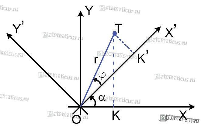
Пусть точка T в новой полярной системе координат имеет полярный радиус r и полярный угол φ. В старой полярной системе координат полярный угол точки T будет равен α+φ, а полярный радиус r будет как в новой системе координат.
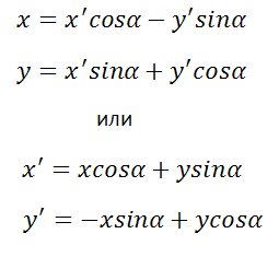
Тогда уравнения примут вид:
x = r cos(α+φ)
y = r sin(α+φ)
Применяя тригонометрические тождества суммы двух углов для синуса и косинуса , получим выражения:
x = r (cosα cosφ — sinα sinφ) = r (cosφ) cosα — (r sinφ) sinα
y = r (sinα cosφ + cosα sinφ) = r (cosφ) sinα + (r sinφ) cosα
Обозначим
X = r cosφ и Y = r sinφ
Получим уравнения поворота осей координат
x = X cosα — Y sinα
y = X sinα + Y cosα
Если обозначим следующим образом
x = OK , y = KT — старые координаты точки T
x´= OK´, y´ = KT´ — новые координаты точки T
α — угол поворота осей
тогда формулы поворота осей координат примут вид:
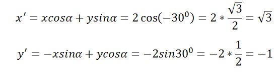
Пример
До поворота осей на угол -300 точка L имела абсциссу x=2 и ординату y=0
Требуется найти координаты точки L после поворота осей.
Решение
Подставляя в формулу, находим новые координаты осей x´, y´
![]() 12868
12868
В
аналитической геометрии часто применяется
преобразование координат, называемое
поворотом
осей. Оно
заключается в следующем: обе оси координат
поворачиваются в одну сторону на один
и тот же угол, а начало координат остается
неизменным. Примеры использования этого
преобразования будут даны в следующих
двух параграфах.
Пусть
оси координат повернуты на угол
(рис. 3.14). Угол
– это угол, на который нужно повернуть
старую ось
до ее совмещения с новой осью
![]()
;
угол
считается положительным при повороте
против часовой стрелки.
Выведем
формулы, позволяющие выразить старые
координаты
и
любой точки
через ее новые координаты
![]()
и
![]()
.
Для
этого построим радиус-вектор
![]()
точки
и обозначим через
![]()
и
![]()
углы, образованные им соответственно
с осями
и
:
точка
имеет полярные координаты
![]()
и
,
если за полярную ось принять ось
,
и координаты
и
,
если за полярную ось принять ось
.
Углы
,
и
связаны равенством
![]()
.
Выражая декартовы координаты точки
через ее полярные координаты, имеем:
![]()
(А)
![]()
(Б)
Заменяя
в формулах (А)
на
![]()
и используя формулы для синуса и косинуса
суммы двух углов, находим:
![]()
,
![]()
.
Отсюда,
используя формулы (Б), находим следующие
формулы, выражающие старые координаты
и
через
новые координаты
и
:
![]()
(3.42)
,
![]()
.
Формулы обратного
перехода, выражающие новые координаты
через старые, мы получим аналогичным
путем из формул (Б), заменяя в них угол
на
![]()
:
![]()
(3.42′)
,
![]()
.
Формулы
(3.42′)
можно получить также из соотношений
(3.42), рассматривая их как уравнения,
определяющие
и
через
и
,
и разрешая их относительно
и
.
Формулы
(3.42′)
можно было бы получить из формул (3.42)
еще и следующим путем: поменять в формулах
(3.42) местами
и
,
а также
и
и заменить
на
![]()
(так как новые оси получаются из старых
поворотом на угол
,
то и старые оси могут быть получены из
новых поворотом в обратную сторону, т.
е. на угол
).
Рекомендуем
читателю получить формулы (3.42′)
этими двумя способами.
§ 3.9. Исследование общего уравнения кривой второго порядка Наиболее общее уравнение второй степени относительно и имеет вид:
(3.49)
![]()
.
В
аналитической геометрии его называют
общим уравнением кривой второго порядка.
От уравнения:
![]()
уравнение
(3.49) отличается наличием члена с
произведением координат, т. е. коэффициент
![]()
мы считаем не равным нулю.
В
настоящем параграфе наша задача –
показать, что и уравнение (3.49), так же,
как и уравнение (3.39), может определять
только одну из изученных нами ранее
кривых – эллипс, гиперболу или параболу
(с возможными для каждого из них случаями
вырождения), найти способ по виду
уравнения (3.49) установить тип определяемой
им кривой (подобно тому, как это делалось
для уравнения (3.39) по знаку произведения
![]()
)
и научиться для каждого конкретного
уравнения (3.49) строить кривую.
Наиболее
простой способ решения этой задачи –
при помощи поворота координатных осей
на некоторый угол
преобразовать уравнение (3.49) в уравнение
вида (3.39) по отношению к новой системе
координат, поскольку уравнение (3.39) нами
уже изучено во всех подробностях.
Итак,
повернем координатные оси на некоторый
угол
.
Новые оси координат обозначим через
и
![]()
.
Тогда старые координаты будут выражаться
через новые по формулам (3.42) так:
,
.
Подставляя
эти значения
и
в уравнение (3.49), после приведения
подобных членов приведем его к виду:
(3.50)
Уравнение (3.50) имеет
ту же структуру, что и уравнение (3.49).
его можно записать в виде:
(3.50′)
![]()
где
![]()
(3.51)
(Значения
новых коэффициентов
![]()
и
![]()
,
несущественные для дальнейшего, мы не
описываем.)
Выберем
теперь угол
таким, чтобы новый коэффициент
в уравнении (3.50′)
обратился бы в нуль; это дает нам для
определения угла
уравнение:
![]()
(3.52)
,
откуда
находим:
![]()
(3.53)
.
Формула
(3.53) определяет два значения угла
,
разность между которыми равна
;
поэтому безразлично, какое из них
выбрать: переход от одного к другому
равносилен перестановке новых осей
координат
и
.
После
того, как угол
определен по формуле (3.53), уравнение
(3.50′)
приводится к виду:
(3.54)
![]()
и,
как нам известно, определяет эллипс
(окружность), гиперболу или параболу
(или вырождения этих кривых) в зависимости
от знака произведения
![]()
(см. § 3.6.).
Соседние файлы в предмете [НЕСОРТИРОВАННОЕ]
- #
- #
- #
- #
- #
- #
- #
- #
- #
- #
- #


-
Линейная алгебра
Расчёт углов поворота между двумя системами координат
Есть ортогональная трёхмерная система координат (OXYZ). Есть другая ортогональная система координат (OX`Y`Z`), повёрнутая относительно первой на неизвестные углы. Центры систем координат совпадают. В системе координат (OXYZ) мы знаем координаты вектора OX` и вектора OZ`. Необходимо найти матрицу поворота для перехода из системы координат (OXYZ) в (OX`Y`Z`). Помогайте, а то весь мозг себе сломал. Или подскажите в какую сторону копать.
-
Вопрос заданболее трёх лет назад
-
22404 просмотра
1
комментарий
-
Столкнулся с очень похожей проблемой. Вопрос автору. Так какое же решение подошло наилучшим образом?
Решения вопроса 1

ОМГ, в шоке от ответов про кватернионы ))
Если координаты в XYZ
OX’ = (x1, y1, z1)
OY’ = (x2, y2, z2)
OZ’ = (x3, y3, z3)
То матрица преобразования из XYZ в X`Y`Z`
x1, x2, x3
y1, y2, y3
z1, z2, z3
Собственно практически по определению
-
Максим
@R6MF49T2 Автор вопроса
Всё же получится матрица преобразования из X`Y`Z` в XYZ. Но по условию задачи известны координаты только осей OX’ и OZ’. Координаты OY’ не известны.
-
Максим
@R6MF49T2 Автор вопроса
Но всё равно спаибо, можно попробовать посчитать координаты третей оси, так как решение с поворотами до совмещение осей дало громадную результирующую матрицу поворота.
-
координаты 3-й оси — это векторное произведение первых двух
Пригласить эксперта
Ответы на вопрос 5

Извините, если я сейчас ошибаюсь, но у вас будет две матрицы поворота. Вокруг оси X и вокруг оси Y. Вот они:
Вокруг X:

Вокруг Y:

Ну, а найти углы поворотов это элементарно:

Ведь у вас есть координаты OX` и OY` в исходной системе.
-
Максим
@R6MF49T2 Автор вопроса
по идее если по матрице перехода пересчитать допустим ось OX то она должна совпасть с осью OX’. как это сделать без поворота вокруг оси OZ я не представляю. В моём понимании должно быть как минимум 3 поворота.
-
Поворот по двум осям задает угол поворота по третей единственным образом.
-
Максим
@R6MF49T2 Автор вопроса
Хорошо, вот только не понял углы поворота фи и пси между чем и чем? Лично мне их найти не так элементарно как вам и я не понимаю что за формулу вы дали.
-
Угол фи, это угол между векторами OX и OX`, угол пси это угол между OY и OY`. Что бы их найти нужно подставить соответствующие векторы в формулу и вычислить арккосинус от того, что получится.
-
Максим
@R6MF49T2 Автор вопроса
теперь понятно. Вот только всё же в первом сообщении вы пишете о повороте вокруг оси X и Y. А если угол фи это угол между векторами OX и OX` то вращать нам надо всё же вокруг OY’ для совмещения OX и OX`. Обозначим эту новую повёрнутую систему как OX«Y»Z». для совмещения осей OY и OY» расчитываем угол между ними и поворачиваем вокруг оси OX», она же OX’. Так?

-
Максим
@R6MF49T2 Автор вопроса
Что такое кватернион я знаю. Проблема здесь не выполнить поворот, а определить оси вращения и углы на которые нужно выполнять поворот.
-
Поворачиваем систему координат сперва так, чтобы совпал OX’ с OX, при этом OY’ переходит в, скажем, OY». Потом повернутую систему поворачиваем второй раз (вокруг OX’) чтобы OY» совпал с OY. (При первом повороте ось вращения получим как векторное произведение OX’ и OX, а угол поворота — в обоих случаях — через скалярное, формулу уже привели выше.) Оба поворота выразим кватернионами, и потом из их композиции и получим и ось, и угол.
-
Максим
@R6MF49T2 Автор вопроса
так как мы рассчитываем переход из системы OXYZ к OX’Y’Z’ то соответственно предлагаю доворачивать OXYZ до OX’Y’Z’ а не наоборот. Итак вначале по формуле
рассчитываем угол между OX и OX’ и поворочиваетм по оси OY’. при этом у нас совпадут OX’ и OX Повёрнутую систему обзовём OX«Y»Z». Теперь чтобы совместить OY’ и OY» находим между ними угол и поворачиваем вдоль оси OX», он же OX’. Так? -
Да, верно — второй поворот делать вокруг того вектора, который уже совмещен. Но чтобы совместить его первым поворотом, векторное произведение посчитать, в общем случае, всё же нужно. И использовать это векторное произведение как ось вращения для первого поворота. Разве что, по условиям задачи, OY’ — это нормаль к плоскости XOX’?
P.S.: Случайно изменил обозначения по сравнению с теми, что были в вопросе. В вопросе — векторы OX’ и OZ’, а у меня — OX’ и OY’.
 рассчитываем угол между OX и OX’ и поворочиваетм по оси OY’. при этом у нас совпадут OX’ и OX Повёрнутую систему обзовём OX«Y»Z». Теперь чтобы совместить OY’ и OY» находим между ними угол и поворачиваем вдоль оси OX», он же OX’. Так?
 Насколько я могу припомнить, если мы возьмём координаты ортов новой системы, помещённых в старую, то эти координаты и будут строками искомой матрицы.
-
Максим
@R6MF49T2 Автор вопроса
Точно строками? Предположим что новая система координат отличается от старой только поворотом вокруг оси y на 45 градусов. тогда если верить вашим словам матрица поворота примет вид:
0.7, 0, 0.7
0, 0, 0
-0.7, 0, 0.7умножим на эту матрицу вектор OX
1
0
0и получим вектор с координатами 0.7, 0, -0.7. А должны были 0.7, 0, 0.7.
-
Значит, столбцами — зависит от формы записи. Мне приходилось иметь дело с обоими вариантами, так что сразу не сориентировался, что требуется для классического варианта. Кстати, второй вектор будет всё же (0, 1, 0).

@VoidVolker
Разработчик ПО и IT-инженер

Похожие вопросы
-
Показать ещё
Загружается…
30 мая 2023, в 00:55
125000 руб./за проект
30 мая 2023, в 00:34
1000 руб./за проект
29 мая 2023, в 23:21
2000 руб./за проект
Минуточку внимания
Исходим из уравнения
![]() (1)
(1)
И покажем, что всегда можно выбрать угол поворота ![]() координатных осей так, что «смешанный» член
координатных осей так, что «смешанный» член ![]() обратится в нуль. Пусть система координат X»O’y» получена поворотом системы X’O’y’ вокруг начала O’ на угол
обратится в нуль. Пусть система координат X»O’y» получена поворотом системы X’O’y’ вокруг начала O’ на угол ![]() .
.
Как видно из рисунка, «старые» и «новые» координаты связаны равенствами
![]() (2)
(2)
Подставим их в уравнение (1)
 Последнюю квадратную скобку перепишем в виде
 ![]() и выберем угол j так, чтобы она обращалась в нуль:
и выберем угол j так, чтобы она обращалась в нуль:
![]() .
.
Разделим это уравнение на ![]() , получим
, получим ![]() . Откуда найдем искомый угол
. Откуда найдем искомый угол
![]() . (3)
. (3)
Обозначая в (2) первые квадратные скобки ![]() , а вторые
, а вторые ![]() , получим уравнение (20.4) в «новой» системе координат
, получим уравнение (20.4) в «новой» системе координат
![]() . (4)
. (4)
ВЫВОД: Для кривой, заданной уравнением (1), поворотом осей координат можно «уничтожить» смешанный (билинейный) член и преобразовать его к уравнению (4); при этом свободный член не изменяется.
Пример 1. Поворотом осей координат установить тип кривой, заданной уравнением
![]() .
.
Сравнивая с уравнением (20.4), находим
![]() .
.
По формуле (3) найдем угол поворота ![]() .
.
Итак, для приведения кривой к каноническому виду следует сделать поворот осей на угол ![]() , при этом формулы перехода даются (2):
, при этом формулы перехода даются (2):

Подставим эти значения в исходное уравнение, получим
![]() .
.
Разделим уравнение на свободный член и перенесем его в правую часть уравнения, получим ![]() — это эллипс с полуосями
— это эллипс с полуосями ![]() .
.
| < Предыдущая | Следующая > |
|---|