Цель: ознакомить учащихся с правилами сложения и умножения вероятностей, понятием противоположных событий на кругах Эйлера.
Теория вероятностей есть математическая наука, изучающая закономерности в случайных явлениях.
Случайное явление – это такое явление, которое при неоднократном воспроизведении одного и того же опыта протекает каждый раз несколько по иному.
Приведём примеры случайных событий: бросаются игральные кости, бросается монета, проводится стрельба по мишени и т.д.
Все приведённые примеры можно рассматривать под одним и тем же углом зрения: случайные вариации, неодинаковые результаты ряда опытов, основные условия которых остаются неизменными.
Совершенно очевидно, что в природе нет ни одного физического явления, в котором не присутствовали бы в той или иной степени элементы случайности. Как бы точно и подробно ни были фиксированы условия опыта, невозможно достигнуть того, чтобы при повторении опыта результаты полностью и в точности совпадали.
Случайные отклонения неизбежно сопутствуют любому закономерному явлению. Тем не менее, в ряде практических задач этими случайными элементами можно пренебречь, рассматривая вместо реального явления, его упрощённую схему «модель» и предполагая, что в данных условиях опыта явление протекает вполне определённым образом.
Однако существует ряд задач, где интересующий нас исход опыта зависит от столь большого числа факторов, что практически невозможно зарегистрировать и учесть все эти факторы.
Случайные события можно различным способом сочетать друг с другом. При этом образуются новые случайные события.
Для наглядного изображения событий используют диаграммы Эйлера. На каждой такой диаграмме прямоугольником изображают множество всех элементарных событий (рис.1). Все другие события изображают внутри прямоугольника в виде некоторой его части, ограниченной замкнутой линией. Обычно такие события изображают окружности или овалы внутри прямоугольника.
Рис.1
Рассмотрим наиболее важные свойства событий с помощью диаграмм Эйлера.
Объединением событий A и B называют событие C, состоящее из элементарных событий принадлежащих событию А или В (иногда объединения называют суммой).
![]()
Результат объединения можно изобразить графически диаграммой Эйлера (рис. 2).
Рис.2
Пересечением событий А и В называют событие С, которое благоприятствует и событию А, и событию В (иногда пересечения называют произведением).
![]()
Результат пересечения можно изобразить графически диаграммой Эйлера (рис. 3).
Рис.3
Если события А и В не имеют общих благоприятствующих элементарных событий, то они не могут наступить одновременно в ходе одного и то же опыта. Такие события называют несовместными, а их пересечение – пустое событие.
Разностью событий А и В называют событие С, состоящее из элементарных событий А, которые не являются элементарными событиями В.
![]()
Результат разности можно изобразить графически диаграммой Эйлера (рис.4)
Рис.4
Пусть прямоугольник изображает все элементарные события. Событие А изобразим в виде круга внутри прямоугольника. Оставшаяся часть прямоугольника изображает противоположное событию ![]() A, событие
A, событие ![]() (рис.5)
(рис.5)
Событием, противоположным событию А называют событие, которому благоприятствуют все элементарные события, не благоприятствующие событию А.
Событие, противоположное событию А, принято обозначать ![]() .
.
Рис.5
Примеры противоположных событий.
- А — попадание при выстреле,
 — промах при выстреле;
 - В — выпадение герба при бросании монеты, — выпадение цифры при бросании монеты;
- С — безотказная работа всех элементов технической системы,
 — отказ хотя бы одного элемента;
 - D — обнаружение не менее двух бракованных изделий в контрольной партии;
 — обнаружение не более одного бракованного изделия.
Объединением нескольких событий называется событие, состоящее в появлении хотя бы одного из этих событий.
Например, если опыт состоит в пяти выстрелах по мишени и даны события:
А0- ни одного попадания;
А1- ровно одно попадание;
А2- ровно 2 попадания;
А3- ровно 3 попадания;
А4- ровно 4 попадания;
А5- ровно 5 попаданий.
Найти события: не более двух попаданий и не менее трёх попаданий.
Решение: А=А0+А1+А2 – не более двух попаданий;
В=А3+А4+А5 – не менее трёх попаданий.
Пересечением нескольких событий называется событие, состоящее в совместном появлении всех этих событий.
Например, если по мишени производится три выстрела, и рассматриваются события:
В1 — промах при первом выстреле,
В2 — промах при втором выстреле,
ВЗ — промах при третьем выстреле,
то событие ![]() состоит в том, что в мишень не будет ни одного попадания.
состоит в том, что в мишень не будет ни одного попадания.
При определении вероятностей часто приходится представлять сложные события в виде комбинаций более простых событий, применяя и объединение, и пересечение событий.
Например, пусть по мишени производится три выстрела, и рассматриваются следующие элементарные события:
![]() — попадание при первом выстреле,
— попадание при первом выстреле,
![]() — промах при первом выстреле,
— промах при первом выстреле,
![]() — попадание при втором выстреле,
— попадание при втором выстреле,
![]() — промах при втором выстреле,
— промах при втором выстреле,
![]() — попадание при третьем выстреле,
— попадание при третьем выстреле,
![]() — промах при третьем выстреле.
— промах при третьем выстреле.
Рассмотрим более сложное событие В, состоящее в том, что в результате данных трёх выстрелов будет ровно одно попадание в мишень. Событие В можно представить в виде следующей комбинации элементарных событий:
![]()
Событие С, состоящее в том, что в мишень будет не менее двух попаданий, может быть представлено в виде:
![]()
На рис.6.1 и 6.2 показано объединение и пересечение трёх событий.
рис.6
Для определения вероятностей событий применяются не непосредственные прямые методы, а косвенные. Позволяющие по известным вероятностям одних событий определять вероятности других событий, с ними связанных. Применяя эти косвенные методы, мы всегда в той или иной форме пользуемся основными правилами теории вероятностей. Этих правил два: правило сложения вероятностей и правило умножения вероятностей.
Правило сложения вероятностей формулируется следующим образом.
Вероятность объединения двух несовместных событий равна сумме вероятностей этих событий:
Р(А+В) =Р(А)+ Р(В).
Сумма вероятностей противоположных событий равна единице:
Р(А) + Р(![]() )= 1.
)= 1.
На практике весьма часто оказывается легче вычислить вероятность противоположного события А, чем вероятность прямого события А. В этих случаях вычисляют Р (А) и находят
Р (А) = 1-Р(![]() ).
).
Рассмотрим несколько примеров на применение правила сложения.
Пример 1. В лотерее 1000 билетов; из них на один билет падает выигрыш 500 руб., на 10 билетов — выигрыши по 100 руб., на 50 билетов — выигрыши по 20 руб., на 100 — билетов — выигрыши по 5 руб., остальные билеты невыигрышные. Некто покупает один билет. Найти вероятность выиграть не менее 20 руб.
Решение. Рассмотрим события:
А — выиграть не менее 20 руб.,
А1 — выиграть 20 руб.,
А2 — выиграть 100 руб.,
А3 — выиграть 500 руб.
Очевидно, А= А1 +А2+А3.
По правилу сложения вероятностей:
Р (А) = Р (А1) + Р (А2) + Р (А3) = 0,050 + 0,010 + 0,001 = 0,061.
Пример 2. Производится бомбометание по трём складам боеприпасов, причём сбрасывается одна бомба. Вероятность попадания в первый склад 0,01; во второй 0,008; в третий 0,025. При попадании в один из складов взрываются все три. Найти вероятность того, что склады будут взорваны.
Решение. Рассмотрим события:
А — взрыв складов,
А1 — попадание в первый склад,
А2 — попадание во второй склад,
А3 — попадание в третий склад.
Очевидно, А = А1 + А2 + А3.
Так как при сбрасывании одной бомбы события Al, А2, А3 несовместны, то
Р (А) = Р (A1) + Р(А2) +Р(А3) == 0,01 + 0,008 + 0,025 = 0,043.
Пример 3. Круговая мишень состоит из трёх зон: I, II и III. Вероятность попадания в первую зону при одном выстреле 0,15, во вторую 0,23, в третью 0,17. Найти вероятность промаха.

Рис.7
Решение. Обозначим А — промах, ![]() — попадание.
— попадание.
Тогда ![]() =А1+ А2 + А3,
=А1+ А2 + А3,
где А1, А2 , А3 — попадание соответственно в первую, вторую и третью зоны:
Р(![]() ) = Р (A1) + Р (А2) + Р (А3) = 0,15 + 0,23 + 0,17 = 0,55,
) = Р (A1) + Р (А2) + Р (А3) = 0,15 + 0,23 + 0,17 = 0,55,
откуда
Р(А) = 1- Р(![]() ) = 0,45.
) = 0,45.
Операции над событиями. Диаграммы Эйлера – Венна
Содержание
![]()
В теории вероятностей случайными событиями являются подмножества множества элементарных исходов Ω .
Над событиями, как и над любыми множествами, можно совершать следующие операции.
Произведение (пересечение) двух событий
Операцию произведения (пересечения) двух событий A и B обозначают
![]() , или AB, или
, или AB, или ![]() .
.
ОПРЕДЕЛЕНИЕ 1. Произведением (пересечением) двух событий A и B называют такое событие, которое состоит из всех элементов, входящих как в событие A , так и в событие B (рис. 1).
Рис.1
Сумма (объединение) двух событий
Операцию суммы (объединения) двух событий A и B обозначают
A + B или ![]()
ОПРЕДЕЛЕНИЕ 2. Суммой (объединением) двух событий A и B называют такое событие, которое состоит из элементов события A и элементов события B (рис. 2).
Рис.2
Разность двух событий
Операцию разности двух событий A и B обозначают
A B
ОПРЕДЕЛЕНИЕ 3. Разностью событий A и B называют событие, состоящее из тех элементов события A , которые не входят в событие B (рис. 3).
Рис.3
ЗАМЕЧАНИЕ 1. Разностью событий B и A является событие B A , изображенное на рисунке 4.
Рис.4
Симметрическая разность двух событий
Операцию симметрической разности двух событий A и B обозначают
![]()
ОПРЕДЕЛЕНИЕ 4 . Симметрической разностью событий A и B называют событие, состоящее из тех элементов события A , которые не входят в событие B , а также из тех элементов события B , которые не входят в событие A (рис. 5).
Рис.5
Переход к противоположному событию
Событие, противоположное к событию A , обозначают
![]() или AC
или AC
ОПРЕДЕЛЕНИЕ 5. Противоположным событием к событию A называют событие, состоящее из тех элементов всего множества элементарных событий Ω , которые не входят в событие A (рис. 6).
Рис.6
ЗАМЕЧАНИЕ 2. Справедлива формула
![]()
ОПРЕДЕЛЕНИЕ 6. Событие Ω называют достоверным событием, пустое множество ![]() называют невозможным событием.
называют невозможным событием.
ЗАМЕЧАНИЕ 3. Рисунки, на которых наглядно показаны операции над множествами, называют диаграммами Эйлера-Венна. В частности, диаграммами Эйлера-Венна являются рисунки 1-6 .
Можно посчитать двумя способами. Хотя по сути это одно и тоже, но формально различается подсчет.
1-й способ:
Вероятность — это отношение количества благоприятных событий к количеству всех возможных событий.
Условная вероятность Р(В|А) — это вероятность события В при условии, что А произошло.
Сколько элементарных событий в событии A? Считаем, получаем N=5.
То есть общее количество возможных событий из которых будем выбирать равно 5
Теперь считаем благоприятные события: Должно произойти и событие А и событие B. Таких событий n=3
Искомая вероятность P = n/N = 3/5
2-й способ:
По определению условной вероятности Р(В|А) = P(B∩A)/P(A)
P(B∩A) = 3/10 (три из десяти элементарных событий)
P(A) = 5/10 (пять из десяти элементарных событий)
Р(В|А) = (3/10) : (5/10) = 3/5
Ответ: Р(В|А) = 3/5
In probability theory, conditional probability is a measure of the probability of an event occurring, given that another event (by assumption, presumption, assertion or evidence) has already occurred.[1] This particular method relies on event B occurring with some sort of relationship with another event A. In this event, the event B can be analyzed by a conditional probability with respect to A. If the event of interest is A and the event B is known or assumed to have occurred, «the conditional probability of A given B«, or «the probability of A under the condition B«, is usually written as P(A|B)[2] or occasionally PB(A). This can also be understood as the fraction of probability B that intersects with A:  .[3]
.[3]
For example, the probability that any given person has a cough on any given day may be only 5%. But if we know or assume that the person is sick, then they are much more likely to be coughing. For example, the conditional probability that someone unwell (sick) is coughing might be 75%, in which case we would have that P(Cough) = 5% and P(Cough|Sick) = 75 %. Although there is a relationship between A and B in this example, such a relationship or dependence between A and B is not necessary, nor do they have to occur simultaneously.
P(A|B) may or may not be equal to P(A) (the unconditional probability of A). If P(A|B) = P(A), then events A and B are said to be independent: in such a case, knowledge about either event does not alter the likelihood of each other. P(A|B) (the conditional probability of A given B) typically differs from P(B|A). For example, if a person has dengue fever, the person might have a 90% chance of being tested as positive for the disease. In this case, what is being measured is that if event B (having dengue) has occurred, the probability of A (tested as positive) given that B occurred is 90%, simply writing P(A|B) = 90%. Alternatively, if a person is tested as positive for dengue fever, they may have only a 15% chance of actually having this rare disease due to high false positive rates. In this case, the probability of the event B (having dengue) given that the event A (testing positive) has occurred is 15% or P(B|A) = 15%. It should be apparent now that falsely equating the two probabilities can lead to various errors of reasoning, which is commonly seen through base rate fallacies.
While conditional probabilities can provide extremely useful information, limited information is often supplied or at hand. Therefore, it can be useful to reverse or convert a conditional probability using Bayes’ theorem:  .[4] Another option is to display conditional probabilities in conditional probability table to illuminate the relationship between events.
Definition[edit]

Illustration of conditional probabilities with an Euler diagram. The unconditional probability P(A) = 0.30 + 0.10 + 0.12 = 0.52. However, the conditional probability P(A|B1) = 1, P(A|B2) = 0.12 ÷ (0.12 + 0.04) = 0.75, and P(A|B3) = 0.

On a tree diagram, branch probabilities are conditional on the event associated with the parent node. (Here, the overbars indicate that the event does not occur.)
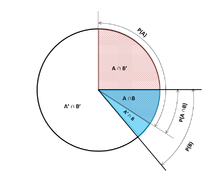
Venn Pie Chart describing conditional probabilities
Conditioning on an event[edit]
Kolmogorov definition[edit]
Given two events A and B from the sigma-field of a probability space, with the unconditional probability of B being greater than zero (i.e., P(B) > 0), the conditional probability of A given B ( ) is the probability of A occurring if B has or is assumed to have happened.[5] A is assumed to be the set of all possible outcomes of an experiment or random trial that has a restricted or reduced sample space. The conditional probability can be found by the quotient of the probability of the joint intersection of events A and B (
 )—the probability at which A and B occur together, although not necessarily occurring at the same time—and the probability of B:[2][6][7]
 .
.
For a sample space consisting of equal likelihood outcomes, the probability of the event A is understood as the fraction of the number of outcomes in A to the number of all outcomes in the sample space. Then, this equation is understood as the fraction of the set  to the set B. Note that the above equation is a definition, not just a theoretical result. We denote the quantity
  as and call it the «conditional probability of A given B.»
As an axiom of probability[edit]
Some authors, such as de Finetti, prefer to introduce conditional probability as an axiom of probability:
- .

This equation for a conditional probability, although mathematically equivalent, may be intuitively easier to understand. It can be interpreted as «the probability of B occurring multiplied by the probability of A occurring, provided that B has occurred, is equal to the probability of the A and B occurrences together, although not necessarily occurring at the same time». Additionally, this may be preferred philosophically; under major probability interpretations, such as the subjective theory, conditional probability is considered a primitive entity. Moreover, this «multiplication rule» can be practically useful in computing the probability of and introduces a symmetry with the summation axiom for Poincaré Formula:
- Thus the equations can be combined to find a new representation of the :


As the probability of a conditional event[edit]
Conditional probability can be defined as the probability of a conditional event  . The Goodman–Nguyen–Van Fraassen conditional event can be defined as:
- , where and represent states or elements of A or B. [8]


It can be shown that

which meets the Kolmogorov definition of conditional probability.[9]
Conditioning on an event of probability zero[edit]
If  , then according to the definition, is undefined.
The case of greatest interest is that of a random variable Y, conditioned on a continuous random variable X resulting in a particular outcome x. The event  has probability zero and, as such, cannot be conditioned on.
Instead of conditioning on X being exactly x, we could condition on it being closer than distance  away from x. The event
  will generally have nonzero probability and hence, can be conditioned on.
We can then take the limit

For example, if two continuous random variables X and Y have a joint density  , then by L’Hôpital’s rule and Leibniz integral rule, upon differentiation with respect to :

The resulting limit is the conditional probability distribution of Y given X and exists when the denominator, the probability density  , is strictly positive.
It is tempting to define the undefined probability  using this limit, but this cannot be done in a consistent manner. In particular, it is possible to find random variables X and W and values x, w such that the events
  and
and  are identical but the resulting limits are not:[10]

The Borel–Kolmogorov paradox demonstrates this with a geometrical argument.
Conditioning on a discrete random variable[edit]
Let X be a discrete random variable and its possible outcomes denoted V. For example, if X represents the value of a rolled die then V is the set  . Let us assume for the sake of presentation that X is a discrete random variable, so that each value in V has a nonzero probability.
For a value x in V and an event A, the conditional probability
is given by .
Writing

for short, we see that it is a function of two variables, x and A.
For a fixed A, we can form the random variable  . It represents an outcome of whenever a value x of X is observed.
The conditional probability of A given X can thus be treated as a random variable Y with outcomes in the interval ![[0,1]](https://wikimedia.org/api/rest_v1/media/math/render/svg/738f7d23bb2d9642bab520020873cccbef49768d) . From the law of total probability, its expected value is equal to the unconditional probability of A.
. From the law of total probability, its expected value is equal to the unconditional probability of A.
Partial conditional probability[edit]
The partial conditional probability

is about the probability of event
 given that each of the condition events
 has occurred to a degree
 (degree of belief, degree of experience) that might be different from 100%. Frequentistically, partial conditional probability makes sense, if the conditions are tested in experiment repetitions of appropriate length
 .[11] Such
-bounded partial conditional probability can be defined as the conditionally expected average occurrence of event
in testbeds of length
that adhere to all of the probability specifications
 , i.e.:
- [11]

Based on that, partial conditional probability can be defined as

where  [11]
[11]
Jeffrey conditionalization[12][13]
is a special case of partial conditional probability, in which the condition events must form a partition:

Example[edit]
Suppose that somebody secretly rolls two fair six-sided dice, and we wish to compute the probability that the face-up value of the first one is 2, given the information that their sum is no greater than 5.
- Let D1 be the value rolled on die 1.
- Let D2 be the value rolled on die 2.
Probability that D1 = 2
Table 1 shows the sample space of 36 combinations of rolled values of the two dice, each of which occurs with probability 1/36, with the numbers displayed in the red and dark gray cells being D1 + D2.
D1 = 2 in exactly 6 of the 36 outcomes; thus P(D1 = 2) = 6⁄36 = 1⁄6:
-
Table 1
+ D2 1 2 3 4 5 6 D1 1 2 3 4 5 6 7 2 3 4 5 6 7 8 3 4 5 6 7 8 9 4 5 6 7 8 9 10 5 6 7 8 9 10 11 6 7 8 9 10 11 12
Probability that D1 + D2 ≤ 5
Table 2 shows that D1 + D2 ≤ 5 for exactly 10 of the 36 outcomes, thus P(D1 + D2 ≤ 5) = 10⁄36:
-
Table 2
+ D2 1 2 3 4 5 6 D1 1 2 3 4 5 6 7 2 3 4 5 6 7 8 3 4 5 6 7 8 9 4 5 6 7 8 9 10 5 6 7 8 9 10 11 6 7 8 9 10 11 12
Probability that D1 = 2 given that D1 + D2 ≤ 5
Table 3 shows that for 3 of these 10 outcomes, D1 = 2.
Thus, the conditional probability P(D1 = 2 | D1+D2 ≤ 5) = 3⁄10 = 0.3:
-
Table 3
+ D2 1 2 3 4 5 6 D1 1 2 3 4 5 6 7 2 3 4 5 6 7 8 3 4 5 6 7 8 9 4 5 6 7 8 9 10 5 6 7 8 9 10 11 6 7 8 9 10 11 12
Here, in the earlier notation for the definition of conditional probability, the conditioning event B is that D1 + D2 ≤ 5, and the event A is D1 = 2. We have  as seen in the table.
Use in inference[edit]
In statistical inference, the conditional probability is an update of the probability of an event based on new information.[14] The new information can be incorporated as follows:[1]
This approach results in a probability measure that is consistent with the original probability measure and satisfies all the Kolmogorov axioms. This conditional probability measure also could have resulted by assuming that the relative magnitude of the probability of A with respect to X will be preserved with respect to B (cf. a Formal Derivation below).
The wording «evidence» or «information» is generally used in the Bayesian interpretation of probability. The conditioning event is interpreted as evidence for the conditioned event. That is, P(A) is the probability of A before accounting for evidence E, and P(A|E) is the probability of A after having accounted for evidence E or after having updated P(A). This is consistent with the frequentist interpretation, which is the first definition given above.
Example[edit]
When Morse code is transmitted, there is a certain probability that the «dot» or «dash» that was received is erroneous. This is often taken as interference in the transmission of a message. Therefore, it is important to consider when sending a «dot», for example, the probability that a «dot» was received. This is represented by:  In Morse code, the ratio of dots to dashes is 3:4 at the point of sending, so the probability of a «dot» and «dash» are
  . If it is assumed that the probability that a dot is transmitted as a dash is 1/10, and that the probability that a dash is transmitted as a dot is likewise 1/10, then Bayes’s rule can be used to calculate
  .
.


Now,  can be calculated:
 [15]
[15]
Statistical independence[edit]
Events A and B are defined to be statistically independent if the probability of the intersection of A and B is equal to the product of the probabilities of A and B:

If P(B) is not zero, then this is equivalent to the statement that

Similarly, if P(A) is not zero, then

is also equivalent. Although the derived forms may seem more intuitive, they are not the preferred definition as the conditional probabilities may be undefined, and the preferred definition is symmetrical in A and B. Independence does not refer to a disjoint event.[16]
It should also be noted that given the independent event pair [A B] and an event C, the pair is defined to be conditionally independent if the product holds true:[17]

This theorem could be useful in applications where multiple independent events are being observed.
Independent events vs. mutually exclusive events
The concepts of mutually independent events and mutually exclusive events are separate and distinct. The following table contrasts results for the two cases (provided that the probability of the conditioning event is not zero).
| If statistically independent | If mutually exclusive | |
|---|---|---|

|

|
0 |

|

|
0 |

|

|
0 |
In fact, mutually exclusive events cannot be statistically independent (unless both of them are impossible), since knowing that one occurs gives information about the other (in particular, that the latter will certainly not occur).
Common fallacies[edit]
- These fallacies should not be confused with Robert K. Shope’s 1978 «conditional fallacy», which deals with counterfactual examples that beg the question.
Assuming conditional probability is of similar size to its inverse[edit]
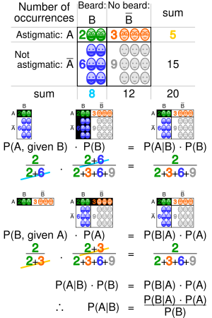
A geometric visualization of Bayes’ theorem. In the table, the values 2, 3, 6 and 9 give the relative weights of each corresponding condition and case. The figures denote the cells of the table involved in each metric, the probability being the fraction of each figure that is shaded. This shows that P(A|B) P(B) = P(B|A) P(A) i.e. P(A|B) = P(B|A) P(A)/P(B) . Similar reasoning can be used to show that P(Ā|B) =
P(B|Ā) P(Ā)/P(B) etc.
In general, it cannot be assumed that P(A|B) ≈ P(B|A). This can be an insidious error, even for those who are highly conversant with statistics.[18] The relationship between P(A|B) and P(B|A) is given by Bayes’ theorem:

That is, P(A|B) ≈ P(B|A) only if P(B)/P(A) ≈ 1, or equivalently, P(A) ≈ P(B).
Assuming marginal and conditional probabilities are of similar size[edit]
In general, it cannot be assumed that P(A) ≈ P(A|B). These probabilities are linked through the law of total probability:

where the events  form a countable partition of
  .
.
This fallacy may arise through selection bias.[19] For example, in the context of a medical claim, let SC be the event that a sequela (chronic disease) S occurs as a consequence of circumstance (acute condition) C. Let H be the event that an individual seeks medical help. Suppose that in most cases, C does not cause S (so that P(SC) is low). Suppose also that medical attention is only sought if S has occurred due to C. From experience of patients, a doctor may therefore erroneously conclude that P(SC) is high. The actual probability observed by the doctor is P(SC|H).
Over- or under-weighting priors[edit]
Not taking prior probability into account partially or completely is called base rate neglect. The reverse, insufficient adjustment from the prior probability is conservatism.
Formal derivation[edit]
Formally, P(A | B) is defined as the probability of A according to a new probability function on the sample space, such that outcomes not in B have probability 0 and that it is consistent with all original probability measures.[20][21]
Let Ω be a discrete sample space with elementary events {ω}, and let P be the probability measure with respect to the σ-algebra of Ω. Suppose we are told that the event B ⊆ Ω has occurred. A new probability distribution (denoted by the conditional notation) is to be assigned on {ω} to reflect this. All events that are not in B will have null probability in the new distribution. For events in B, two conditions must be met: the probability of B is one and the relative magnitudes of the probabilities must be preserved. The former is required by the axioms of probability, and the latter stems from the fact that the new probability measure has to be the analog of P in which the probability of B is one — and every event that is not in B, therefore, has a null probability. Hence, for some scale factor α, the new distribution must satisfy:


Substituting 1 and 2 into 3 to select α:
![{displaystyle {begin{aligned}1&=sum _{omega in Omega }{P(omega mid B)}\&=sum _{omega in B}{P(omega mid B)}+{cancelto {0}{sum _{omega notin B}P(omega mid B)}}\&=alpha sum _{omega in B}{P(omega )}\[5pt]&=alpha cdot P(B)\[5pt]Rightarrow alpha &={frac {1}{P(B)}}end{aligned}}}](https://wikimedia.org/api/rest_v1/media/math/render/svg/bc21b49c38af5566aeb4794016be9ee06b40458c)
So the new probability distribution is

Now for a general event A,
![{displaystyle {begin{aligned}P(Amid B)&=sum _{omega in Acap B}{P(omega mid B)}+{cancelto {0}{sum _{omega in Acap B^{c}}P(omega mid B)}}\&=sum _{omega in Acap B}{frac {P(omega )}{P(B)}}\[5pt]&={frac {P(Acap B)}{P(B)}}end{aligned}}}](https://wikimedia.org/api/rest_v1/media/math/render/svg/4f6e98f9200e5cf74a15231fc3c753ccfeb8d1c6)
See also[edit]
- Bayes’ theorem
- Bayesian epistemology
- Borel–Kolmogorov paradox
- Chain rule (probability)
- Class membership probabilities
- Conditional independence
- Conditional probability distribution
- Conditioning (probability)
- Joint probability distribution
- Monty Hall problem
- Pairwise independent distribution
- Posterior probability
- Regular conditional probability
References[edit]
- ^ a b Gut, Allan (2013). Probability: A Graduate Course (Second ed.). New York, NY: Springer. ISBN 978-1-4614-4707-8.
- ^ a b «Conditional Probability». www.mathsisfun.com. Retrieved 2020-09-11.
- ^ Dekking, Frederik Michel; Kraaikamp, Cornelis; Lopuhaä, Hendrik Paul; Meester, Ludolf Erwin (2005). «A Modern Introduction to Probability and Statistics». Springer Texts in Statistics: 26. doi:10.1007/1-84628-168-7. ISBN 978-1-85233-896-1. ISSN 1431-875X.
- ^ Dekking, Frederik Michel; Kraaikamp, Cornelis; Lopuhaä, Hendrik Paul; Meester, Ludolf Erwin (2005). «A Modern Introduction to Probability and Statistics». Springer Texts in Statistics: 25–40. doi:10.1007/1-84628-168-7. ISBN 978-1-85233-896-1. ISSN 1431-875X.
- ^ Reichl, Linda Elizabeth (2016). «2.3 Probability». A Modern Course in Statistical Physics (4th revised and updated ed.). WILEY-VCH. ISBN 978-3-527-69049-7.
- ^ Kolmogorov, Andrey (1956), Foundations of the Theory of Probability, Chelsea
- ^ «Conditional Probability». www.stat.yale.edu. Retrieved 2020-09-11.
- ^ Flaminio, Tommaso; Godo, Lluis; Hosni, Hykel (2020-09-01). «Boolean algebras of conditionals, probability and logic». Artificial Intelligence. 286: 103347. arXiv:2006.04673. doi:10.1016/j.artint.2020.103347. ISSN 0004-3702. S2CID 214584872.
- ^ Van Fraassen, Bas C. (1976), Harper, William L.; Hooker, Clifford Alan (eds.), «Probabilities of Conditionals», Foundations of Probability Theory, Statistical Inference, and Statistical Theories of Science: Volume I Foundations and Philosophy of Epistemic Applications of Probability Theory, The University of Western Ontario Series in Philosophy of Science, Dordrecht: Springer Netherlands, pp. 261–308, doi:10.1007/978-94-010-1853-1_10, ISBN 978-94-010-1853-1, retrieved 2021-12-04
- ^ Gal, Yarin. «The Borel–Kolmogorov paradox» (PDF).
- ^ a b c Draheim, Dirk (2017). «Generalized Jeffrey Conditionalization (A Frequentist Semantics of Partial Conditionalization)». Springer. Retrieved December 19, 2017.
- ^ Jeffrey, Richard C. (1983), The Logic of Decision, 2nd edition, University of Chicago Press, ISBN 9780226395821
- ^ «Bayesian Epistemology». Stanford Encyclopedia of Philosophy. 2017. Retrieved December 29, 2017.
- ^ Casella, George; Berger, Roger L. (2002). Statistical Inference. Duxbury Press. ISBN 0-534-24312-6.
- ^ «Conditional Probability and Independence» (PDF). Retrieved 2021-12-22.
- ^ Tijms, Henk (2012). Understanding Probability (3 ed.). Cambridge: Cambridge University Press. doi:10.1017/cbo9781139206990. ISBN 978-1-107-65856-1.
- ^ Pfeiffer, Paul E. (1978). Conditional Independence in Applied Probability. Boston, MA: Birkhäuser Boston. ISBN 978-1-4612-6335-7. OCLC 858880328.
- ^ Paulos, J.A. (1988) Innumeracy: Mathematical Illiteracy and its Consequences, Hill and Wang. ISBN 0-8090-7447-8 (p. 63 et seq.)
- ^ F. Thomas Bruss Der Wyatt-Earp-Effekt oder die betörende Macht kleiner Wahrscheinlichkeiten (in German), Spektrum der Wissenschaft (German Edition of Scientific American), Vol 2, 110–113, (2007).
- ^ George Casella and Roger L. Berger (1990), Statistical Inference, Duxbury Press, ISBN 0-534-11958-1 (p. 18 et seq.)
- ^ Grinstead and Snell’s Introduction to Probability, p. 134
External links[edit]
- Weisstein, Eric W. «Conditional Probability». MathWorld.
- Visual explanation of conditional probability
Операции над событиями
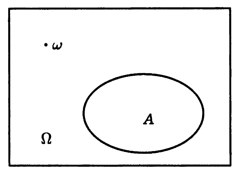
Рис. 1. Изображение диаграммы
Эйлера-Венна
Часто бывает полезно наглядно представить события в виде диаграммы Эйлера — Венна. Изобразим все пространство элементарных исходов прямоугольником (рис. 1). При этом, каждый элементарный исход %%omega%% соответствует точке внутри прямоугольника, а каждое событие %%A%% — некоторому множеству точек, этого прямоугольника.
Рассмотрим теперь операции над событиями, которые совпадают с операциями над множествами.
Определение
Пересечением (произведением) двух событий %%A%% и %%B%% называют событие, обозначаемое %%A cap B%% или %%AB%%, происходящее тогда и только тогда, когда одновременно происходят оба события %%A%% и %%B%%, т.е. событие, состоящее из тех и только тех элементарных исходов, которые принадлежат и событию %%A%%, и событию %%B%%.
События %%A%% и %%B%% называются несовместными, или непересекающимися, если их пересечение является невозможным событием, т.е. если %%A cap B = varnothing%%.
В противном случае события называют совместными, или пересекающимися.
Определение
Объединением (суммой) двух событий %%A%% и %%B%% называют событие, обозначаемое %%A cup B%%, происходящее тогда и только тогда, когда происходит хотя бы одно из событий %%A%% или %%B%%, т.е. событие состоит из элементарных исходов, которые принадлежат хотя бы одному из множеств %%A%% или %%B%%.
Если события %%A%% и %%B%% несовместимы, то для обозначения могут использововать символ «%%+%%».
Например, поскольку невозможное событие %%varnothing%% несовместно с любым событием %%A%%, то
$$
varnothing cup A = varnothing + A = A.
$$
Аналогично определяют понятия произведения и суммы событий для любого конечного числа событий и даже для бесконечных последовательностей событий. Так, событие
$$
A_1 A_2 ldots A_n = bigcap_{i = 1}^n A_i
$$
состоит из элементарных исходов, принадлежащих всем событиям %%A_i, i = overline{1,n}%%, а событие
$$
A_1 cup A_2 cup ldots cup A_n = bigcup_{i = 1}^n A_i
$$
состоит из элементарных исходов, принадлежащих хотя бы одному из событий %%A_i, i = overline{1,n}%%.
В частности, события %%A_1, A_2, ldots, A_n%% называют попарно несовместными, если
$$
A_i A_j = varnothing
$$
для любых %%i,j = overline{1,n}, i neq j%%, и несовместными в совокупности, если
$$
A_1 A_2 ldots A_n = varnothing.
$$
Определение
Разностью двух событий %%A%% и %%B%% называют событие, обозначаемое %% A setminus B%%, происходящее тогда и только тогда, когда происходит событие %%A%% и не происходит событие %%B%%, т.е. состоит из тех элементарных исходов, которые принадлежат событию %%A%% и не принадлежат событию %%B%%
Определение
Дополнением события %%A%% называют новое событие, обозначаемое %%overline{A}%%, происходящее тогда и только тогда, когда не происходит событие %%A%%. Так событие %%overline{A}%% можно записать в виде:
$$
overline{A} = Omega setminus A.
$$
Событие %%overline{A}%% называют событием, противоположным событию %%A%%.
Определение
Событие %%A%% включено в событие %%B%%, если появление за собой события %%A%% обязательно влечет за собой наступление события %%B%%, или каждый элементарный исход события %%A%% принадлежит и событию %%B%%.
Приоритеты операций
Если некоторое событие записано в виде нескольких операций над различными событиями, то сначала выполняется операция дополнения, затем умножения, и, наконец, сложение и вычитание (слева направо).
Скобки могут увеличить приоритет любой из операций.
Пример
Рассмотрим устройство из %%n%% элементов. Элементы соединены последовательно, если устройство прекращает функционировать при отказе любого из элементов, и соединены параллельно, если прекращение функционирования наступает только при отказе %%n%% элементов (рис. 1а, 1б соответственно).

Рис 1. Последовательное и параллельное соединения
Обозначим %%A%% событие, означающее отказ системы, а %%A_i%% — отказ %%i%%-го элемента (%%i = overline{1,n}%%). Тогда для последовательного соединения событие %%A%% представимо в виде:
$$
A = A_1 cup A_2 cup ldots A_n,
$$
а для параллельного соединения
$$
A = A_1 cap A_2 cap ldots A_n.
$$
Очевидно, что при параллельном соединении элементов событие %%A%% включено в каждое из событий %%A_i, i = overline{1,n}%%, а при последовательном соединении любое событие %%A_i, i = overline{1,n}%% включено в событие %%A%%.