Мультиколлинеарность в регрессионном анализе возникает, когда две или более переменных-предикторов сильно коррелируют друг с другом, так что они не предоставляют уникальную или независимую информацию в регрессионной модели.
Если степень корреляции между переменными достаточно высока, это может вызвать проблемы при подгонке и интерпретации регрессионной модели .
Наиболее распространенным способом обнаружения мультиколлинеарности является использование коэффициента инфляции дисперсии (VIF), который измеряеткорреляцию и силу корреляции между переменными-предикторами в регрессионной модели.
Значение VIF начинается с 1 и не имеет верхнего предела. Общее эмпирическое правило для интерпретации VIF выглядит следующим образом:
- Значение 1 указывает на отсутствие корреляции между данной переменной-предиктором и любыми другими переменными-предикторами в модели.
- Значение от 1 до 5 указывает на умеренную корреляцию между данной переменной-предиктором и другими переменными-предикторами в модели, но часто она недостаточно серьезная, чтобы требовать внимания.
- Значение больше 5 указывает на потенциально сильную корреляцию между данной переменной-предиктором и другими переменными-предикторами в модели. В этом случае оценки коэффициентов и p-значения в выходных данных регрессии, вероятно, ненадежны.
Обратите внимание, что в некоторых случаях высокие значения VIF можно спокойно игнорировать .
Как рассчитать VIF в R
Чтобы проиллюстрировать, как рассчитать VIF для регрессионной модели в R, мы будем использовать встроенный набор данных mtcars :
#view first six lines of *mtcars*
head(mtcars)

# mpg cyl disp hp drat wt qsec vs am gear carb
#Mazda RX4 21.0 6 160 110 3.90 2.620 16.46 0 1 4 4
#Mazda RX4 Wag 21.0 6 160 110 3.90 2.875 17.02 0 1 4 4
#Datsun 710 22.8 4 108 93 3.85 2.320 18.61 1 1 4 1
#Hornet 4 Drive 21.4 6 258 110 3.08 3.215 19.44 1 0 3 1
#Hornet Sportabout 18.7 8 360 175 3.15 3.440 17.02 0 0 3 2
#Valiant 18.1 6 225 105 2.76 3.460 20.22 1 0 3 1
Во-первых, мы подгоним регрессионную модель, используя mpg в качестве переменной ответа и disp , hp , wt и drat в качестве переменных-предикторов:
#fit the regression model
model <- lm(mpg ~ disp + hp + wt + drat, data = mtcars)

#view the output of the regression model
summary(model)

#Call:
#lm(formula = mpg ~ disp + hp + wt + drat, data = mtcars)
#
#Residuals:
# Min 1Q Median 3Q Max
#-3.5077 -1.9052 -0.5057 0.9821 5.6883
#
#Coefficients:
# Estimate Std. Error t value Pr(>|t|)
#(Intercept) 29.148738 6.293588 4.631 8.2e-05 ***
#disp 0.003815 0.010805 0.353 0.72675
#hp -0.034784 0.011597 -2.999 0.00576 **
#wt -3.479668 1.078371 -3.227 0.00327 **
#drat 1.768049 1.319779 1.340 0.19153
#---
#Signif. codes: 0 '***' 0.001 '**' 0.01 '*' 0.05 '.' 0.1 ' ' 1
#
#Residual standard error: 2.602 on 27 degrees of freedom
#Multiple R-squared: 0.8376, Adjusted R-squared: 0.8136
#F-statistic: 34.82 on 4 and 27 DF, p-value: 2.704e-10
Из вывода видно, что значение R-квадрата для модели равно 0,8376.Мы также можем видеть, что общая F-статистика составляет 34,82 , а соответствующее значение p равно 2,704e-10 , что указывает на то, что общая модель регрессии является значимой. Кроме того, переменные-предикторы hp и wt являются статистически значимыми при уровне значимости 0,05, а disp и drat — нет.
Далее мы воспользуемся функцией vif() из библиотеки car , чтобы вычислить VIF для каждой переменной-предиктора в модели:
#load the *car* library
library(car)

#calculate the VIF for each predictor variable in the model
vif(model)

# disp hp wt drat
#8.209402 2.894373 5.096601 2.279547
Мы видим, что VIF для disp и wt больше 5, что потенциально вызывает беспокойство.
Визуализация значений VIF
Чтобы визуализировать значения VIF для каждой переменной-предиктора, мы можем создать простую горизонтальную гистограмму и добавить вертикальную линию на уровне 5, чтобы мы могли четко видеть, какие значения VIF превышают 5:
#create vector of VIF values
vif_values <- vif(model)

#create horizontal bar chart to display each VIF value
barplot(vif_values, main = "VIF Values", horiz = TRUE, col = "steelblue")

#add vertical line at 5
abline(v = 5, lwd = 3, lty = 2)

Обратите внимание, что этот тип диаграммы был бы наиболее полезен для модели с большим количеством переменных-предикторов, поэтому мы могли бы легко визуализировать все значения VIF одновременно. Тем не менее, в этом примере это все еще полезная диаграмма.
В зависимости от того, какое значение VIF вы считаете слишком высоким для включения в модель, вы можете удалить определенные переменные-предикторы и посмотреть, влияет ли это на соответствующее значение R-квадрата или стандартную ошибку модели.
Визуализация корреляций между переменными предиктора
Чтобы лучше понять, почему одна предикторная переменная может иметь высокое значение VIF, мы можем создать матрицу корреляции для просмотра коэффициентов линейной корреляции между каждой парой переменных:
#define the variables we want to include in the correlation matrix
data <- mtcars[ , c("disp", "hp", "wt", "drat")]

#create correlation matrix
cor(data)

# disp hp wt drat
#disp 1.0000000 0.7909486 0.8879799 -0.7102139
#hp 0.7909486 1.0000000 0.6587479 -0.4487591
#wt 0.8879799 0.6587479 1.0000000 -0.7124406
#drat -0.7102139 -0.4487591 -0.7124406 1.0000000
Напомним, что переменная disp имела значение VIF более 8, что было самым большим значением VIF среди всех переменных-предикторов в модели. Из матрицы корреляции видно, что disp сильно коррелирует со всеми тремя другими переменными-предикторами, что объясняет, почему он имеет такое высокое значение VIF.
В этом случае вы можете удалить disp из модели, потому что он имеет высокое значение VIF и не является статистически значимым на уровне значимости 0,05.
Обратите внимание, что корреляционная матрица и VIF предоставят вам аналогичную информацию: они оба сообщают вам, когда одна переменная сильно коррелирует с одной или несколькими другими переменными в регрессионной модели.
Дальнейшее чтение:
Руководство по мультиколлинеарности и VIF в регрессии
Что такое хорошее значение R-квадрата?
Recipe Objective
How to find VIF on a data in R.
When a Linear Regression model is built, there is a chance that some variables can be multicollinear in nature. Multicollinearity is a statistical terminology where more than one independent variable is correlated with each other. This multicollinearity results in reducing the reliability of statistical inferences. Multicollinearity in a regression model analysis occurs when two or more independent predictor variables are highly correlated to each other, which results in the lack of unique information about the regression model. Hence, these variables must be removed when building a multiple regression model. Variance inflation factor (VIF) is used for detecting the multicollinearity in a model, which measures the correlation and strength of correlation between the independent variables in a regression model. — If the value of VIF is less than 1: no correlation — If the value of VIF is between 1-5, there is moderate correlation — If the value of VIF is above 5: severe correlation This recipe demonstrates an example of how to find VIF on a data in R.
Table of Contents
- Recipe Objective
- Step 1 — Install necessary packages
- Step 2 — Define a Dataframe
- Step 3 — Create a linear regression model
- Step 4 — Use the vif() function
- Step 5 — Visualize VIF Values
Step 1 — Install necessary packages
install.packages("caTools")    # For Linear regression

library(caTools)
install.packages('car')
library(car)
Step 2 — Define a Dataframe
data <- data.frame(marks_scored = c(35,42,24,27,37),

                   no_hours_studied = c(5,4,2,3,4),

                   no_hours_played = c(4,3,4,2,2),

                   attendance = c(8,8,4,6,9))
print(data)
"Dataframe is:"
  marks_scored no_hours_studied no_hours_played attendance
1           35                5               4          8
2           42                4               3          8
3           24                2               4          4
4           27                3               2          6
5           37                4               2          9
Step 3 — Create a linear regression model
model_all <- lm(marks_scored ~ ., data=data) # with all the independent variables in the dataframe
summary(model_all)
Step 4 — Use the vif() function
vif(model_all)
"Output of code is:"
no_hours_studied - 9.53333333333337
no_hours_played  - 2.56
attendance       - 11.0933333333334
Step 5 — Visualize VIF Values
vif_values <- vif(model_all) #create vector of VIF values
barplot(vif_values, main = "VIF Values", horiz = TRUE, col = "steelblue") #create horizontal bar chart to display each VIF value
abline(v = 5, lwd = 3, lty = 2) #add vertical line at 5 as after 5 there is severe correlation
After plotting the graph, user can does decide which variable to remove i.e not include in model building and check whether the coreesponding R squared value improves.
{«mode»:»full»,»isActive»:false}
Multicollinearity in regression analysis occurs when two or more predictor variables are highly correlated to each other, such that they do not provide unique or independent information in the regression model.
If the degree of correlation is high enough between variables, it can cause problems when fitting and interpreting the regression model.
The most common way to detect multicollinearity is by using the variance inflation factor (VIF), which measures the correlation and strength of correlation between the predictor variables in a regression model.
The value for VIF starts at 1 and has no upper limit. A general rule of thumb for interpreting VIFs is as follows:
- A value of 1 indicates there is no correlation between a given predictor variable and any other predictor variables in the model.
- A value between 1 and 5 indicates moderate correlation between a given predictor variable and other predictor variables in the model, but this is often not severe enough to require attention.
- A value greater than 5 indicates potentially severe correlation between a given predictor variable and other predictor variables in the model. In this case, the coefficient estimates and p-values in the regression output are likely unreliable.
Note that there are some cases in which high VIF values can safely be ignored.
How to Calculate VIF in R
To illustrate how to calculate VIF for a regression model in R, we will use the built-in dataset mtcars:
#view first six lines of mtcars
head(mtcars)

#                   mpg cyl disp  hp drat    wt  qsec vs am gear carb
#Mazda RX4         21.0   6  160 110 3.90 2.620 16.46  0  1    4    4
#Mazda RX4 Wag     21.0   6  160 110 3.90 2.875 17.02  0  1    4    4
#Datsun 710        22.8   4  108  93 3.85 2.320 18.61  1  1    4    1
#Hornet 4 Drive    21.4   6  258 110 3.08 3.215 19.44  1  0    3    1
#Hornet Sportabout 18.7   8  360 175 3.15 3.440 17.02  0  0    3    2
#Valiant           18.1   6  225 105 2.76 3.460 20.22  1  0    3    1
First, we’ll fit a regression model using mpg as the response variable and disp, hp, wt, and drat as the predictor variables:
#fit the regression model
model <- lm(mpg ~ disp + hp + wt + drat, data = mtcars)

#view the output of the regression model
summary(model)

#Call:
#lm(formula = mpg ~ disp + hp + wt + drat, data = mtcars)
#
#Residuals:
#    Min      1Q  Median      3Q     Max
#-3.5077 -1.9052 -0.5057  0.9821  5.6883
#
#Coefficients:
#             Estimate Std. Error t value Pr(>|t|)
#(Intercept) 29.148738   6.293588   4.631  8.2e-05 ***
#disp         0.003815   0.010805   0.353  0.72675
#hp          -0.034784   0.011597  -2.999  0.00576 **
#wt          -3.479668   1.078371  -3.227  0.00327 **
#drat         1.768049   1.319779   1.340  0.19153
#---
#Signif. codes:  0 '***' 0.001 '**' 0.01 '*' 0.05 '.' 0.1 ' ' 1
#
#Residual standard error: 2.602 on 27 degrees of freedom
#Multiple R-squared:  0.8376,	Adjusted R-squared:  0.8136
#F-statistic: 34.82 on 4 and 27 DF,  p-value: 2.704e-10
We can see from the output that the R-squared value for the model is 0.8376. We can also see that the overall F-statistic is 34.82 and the corresponding p-value is 2.704e-10, which indicates that the overall regression model is significant. Also, the predictor variables hp and wt are statistically significant at the 0.05 significance level while disp and drat are not.
Next, we’ll use the vif() function from the car library to calculate the VIF for each predictor variable in the model:
#load the car library
library(car)

#calculate the VIF for each predictor variable in the model
vif(model)

#    disp       hp       wt     drat
#8.209402 2.894373 5.096601 2.279547
We can see that the VIF for both disp and wt are greater than 5, which is potentially concerning.
Visualizing VIF Values
To visualize the VIF values for each predictor variable, we can create a simple horizontal bar chart and add a vertical line at 5 so we can clearly see which VIF values exceed 5:
#create vector of VIF values
vif_values <- vif(model)

#create horizontal bar chart to display each VIF value
barplot(vif_values, main = "VIF Values", horiz = TRUE, col = "steelblue")

#add vertical line at 5
abline(v = 5, lwd = 3, lty = 2)
Note that this type of chart would be most useful for a model that has a lot of predictor variables, so we could easily visualize all of the VIF values at once. It is still a useful chart in this example, though.
Depending on what value of VIF you deem to be too high to include in the model, you may choose to remove certain predictor variables and see if the corresponding R-squared value or standard error of the model is affected.
Visualizing Correlations Between Predictor Variables
To gain a better understanding of why one predictor variable may have a high VIF value, we can create a correlation matrix to view the linear correlation coefficients between each pair of variables:
#define the variables we want to include in the correlation matrix
data <- mtcars[ , c("disp", "hp", "wt", "drat")]

#create correlation matrix
cor(data)

#           disp         hp         wt       drat
#disp  1.0000000  0.7909486  0.8879799 -0.7102139
#hp    0.7909486  1.0000000  0.6587479 -0.4487591
#wt    0.8879799  0.6587479  1.0000000 -0.7124406
#drat -0.7102139 -0.4487591 -0.7124406  1.0000000
Recall that the variable disp had a VIF value over 8, which was the largest VIF value among all of the predictor variables in the model. From the correlation matrix we can see that disp is strongly correlated with all three of the other predictor variables, which explains why it has such a high VIF value.
In this case, you may want to remove disp from the model because it has a high VIF value and it was not statistically significant at the 0.05 significance level.
Note that a correlation matrix and a VIF will provide you with similar information: they both tell you when one variable is highly correlated with one or more other variables in a regression model.
Further Reading:
A Guide to Multicollinearity & VIF in Regression
What is a Good R-squared Value?
VIF: Variance Inflation Factor
Description
Calculates the variation inflation factors of all predictors in regression models
Usage
VIF(mod)
Arguments
mod
A linear or logistic regression model
Details
This function is a simple port of vif from the car package. The VIF of a predictor is a measure for how easily it is predicted from a linear regression using the other predictors. Taking the square root of the VIF tells you how much larger the standard error of the estimated coefficient is respect to the case when that predictor is independent of the other predictors.
A general guideline is that a VIF larger than 5 or 10 is large, indicating that the model has problems estimating the coefficient. However, this in general does not degrade the quality of predictions. If the VIF is larger than 1/(1-R2), where R2 is the Multiple R-squared of the regression, then that predictor is more related to the other predictors than it is to the response.
References
Introduction to Regression and Modeling with R
Examples
Run this code
# NOT RUN {
	#A case where the VIFs are small
	data(SALARY)
	M <- lm(Salary~.,data=SALARY)
	VIF(M)

  #A case where (some of) the VIFs are large
  data(BODYFAT)
  M <- lm(BodyFat~.,data=BODYFAT)
  VIF(M)

# }
Run the code above in your browser using DataCamp Workspace
To calculate the VIF in R, you can use the “vif()” function from the “car” package.
The Variance Inflation Factor (VIF) measures multicollinearity in multiple regression models. It quantifies the severity of multicollinearity by estimating how much the variance of the estimated regression coefficients is inflated due to multicollinearity.
A VIF value greater than 10 is often considered an indication of high multicollinearity.
if (!requireNamespace("car", quietly = TRUE)) {
  install.packages("car")
}

# Load the libraries
library(car)

model <- lm(mpg ~ disp + hp + wt, data = mtcars)

# Calculate the VIF
vif_values <- vif(model)

# Print the VIF values
print(vif_values)
Output
Loading required package: carData

  disp      hp        wt
7.324517 2.736633  4.844618
The vif() function returns the VIF values for each predictor variable in the regression model.
You can inspect these values to identify potential multicollinearity issues in your model.
Visualizing VIF Values
Visualizing VIF values can help you better understand the presence of multicollinearity in your multiple regression model. One simple way to visualize VIF values is by creating a bar chart.
In this example, we’ll use the ggplot2 package to create a bar chart of VIF values:
if (!requireNamespace("car", quietly = TRUE)) {
  install.packages("car")
}

if (!requireNamespace("ggplot2", quietly = TRUE)) {
  install.packages("ggplot2")
}

# Load the libraries
library(car)
library(ggplot2)

model <- lm(mpg ~ disp + hp + wt, data = mtcars)

# Calculate the VIF
vif_values <- vif(model)

# Create a data frame of the VIF values
vif_data <- data.frame(
  variable = names(vif_values),
  vif = vif_values
)

# Create a bar chart of VIF values
ggplot(vif_data, aes(x = variable, y = vif)) +
  geom_bar(stat = "identity", fill = "steelblue") +
  theme_minimal() +
  geom_hline(yintercept = 10, linetype = "dashed", color = "red") +
  labs(
    title = "Variance Inflation Factor (VIF)",
    x = "Predictor Variables",
    y = "VIF Values"
  )
Output
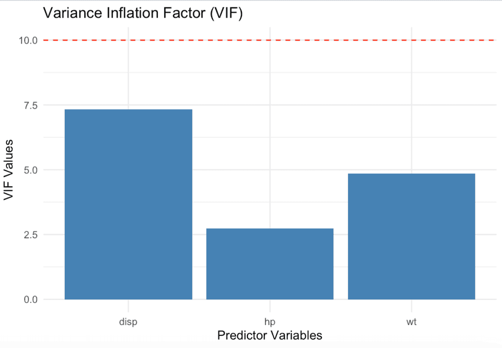
This bar chart displays the VIF values for each predictor variable in the regression model.
The red dashed line at y = 10 serves as a reference to indicate potential multicollinearity issues (values greater than 10 suggest high multicollinearity). That’s it.

Krunal Lathiya is a Software Engineer with over eight years of experience. He has developed a strong foundation in computer science principles and a passion for problem-solving. In addition, Krunal has excellent knowledge of Data Science and Machine Learning, and he is an expert in R Language.
We use cookies on our website to give you the most relevant experience by remembering your preferences and repeat visits. By clicking “Accept”, you consent to the use of ALL the cookies.