Syntax
Description
example
pks = findpeaks(data)
returns a vector with the local maxima (peaks) of the input signal vector,
data. A local peak is a data
sample that is either larger than its two neighboring samples or is equal to
Inf. The peaks are output in order of occurrence.
Non-Inf signal endpoints are excluded. If a peak is flat,
the function returns only the point with the lowest index.
example
[ additionallypks,locs] = findpeaks(data)
returns the indices at which the peaks occur.
example
[ additionally returnspks,locs,w,p]
= findpeaks(data)
the widths of the peaks as the vector w and the
prominences of the peaks as the vector p.
example
[___] = findpeaks( specifies data,x)x as
the location vector and returns any of the output arguments from previous
syntaxes. locs and w are
expressed in terms of x.
example
[___] = findpeaks( specifiesdata,Fs)
the sample rate, Fs, of the data. The first sample
of data is assumed to have been taken at time
zero. locs and w are converted
to time units.
example
[___] = findpeaks(___,Name,Value)
specifies options using name-value arguments in addition to any of the input
arguments in previous syntaxes.
example
findpeaks(___) without output
arguments plots the signal and overlays the peak values.
Examples
collapse all
Find Peaks in a Vector
Define a vector with three peaks and plot it.
data = [25 8 15 5 6 10 10 3 1 20 7];
plot(data)
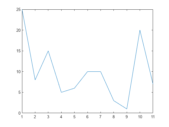
Find the local maxima. The peaks are output in order of occurrence. The first sample is not included despite being the maximum. For the flat peak, the function returns only the point with lowest index.
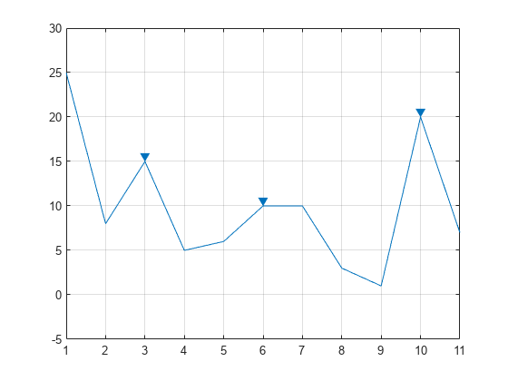
Use findpeaks without output arguments to display the peaks.
Find Peaks and Their Locations
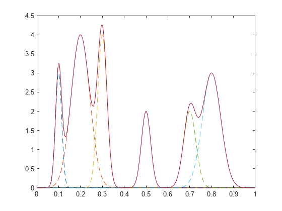
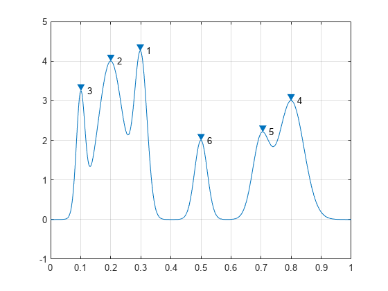
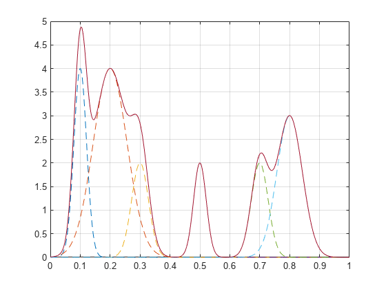
Create a signal that consists of a sum of bell curves. Specify the location, height, and width of each curve.
x = linspace(0,1,1000);

Pos = [1 2 3 5 7 8]/10;
Hgt = [3 4 4 2 2 3];
Wdt = [2 6 3 3 4 6]/100;

for n = 1:length(Pos)
    Gauss(n,:) = Hgt(n)*exp(-((x - Pos(n))/Wdt(n)).^2);
end

PeakSig = sum(Gauss);
Plot the individual curves and their sum.
plot(x,Gauss,'--',x,PeakSig)
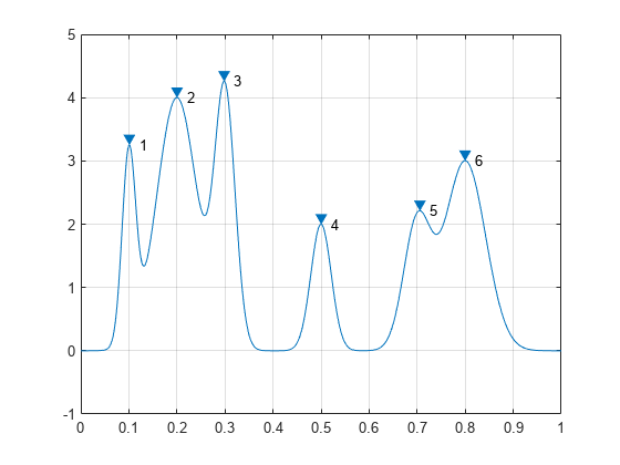
Use findpeaks with default settings to find the peaks of the signal and their locations.
[pks,locs] = findpeaks(PeakSig,x);
Plot the peaks using findpeaks and label them.
findpeaks(PeakSig,x)

text(locs+.02,pks,num2str((1:numel(pks))'))
Sort the peaks from tallest to shortest.
[psor,lsor] = findpeaks(PeakSig,x,'SortStr','descend');

findpeaks(PeakSig,x)

text(lsor+.02,psor,num2str((1:numel(psor))'))
Peak Prominences
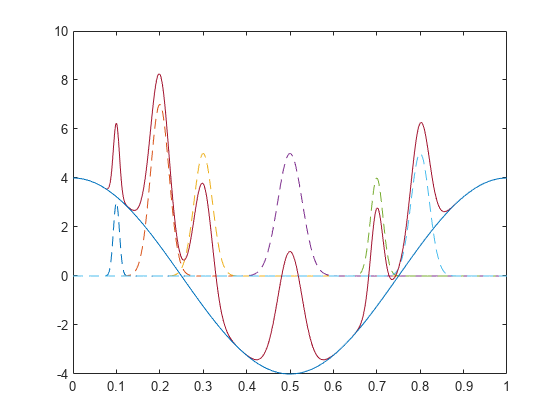
Create a signal that consists of a sum of bell curves riding on a full period of a cosine. Specify the location, height, and width of each curve.
x = linspace(0,1,1000);

base = 4*cos(2*pi*x);

Pos = [1 2 3 5 7 8]/10;
Hgt = [3 7 5 5 4 5];
Wdt = [1 3 3 4 2 3]/100;

for n = 1:length(Pos)
    Gauss(n,:) =  Hgt(n)*exp(-((x - Pos(n))/Wdt(n)).^2);
end

PeakSig = sum(Gauss)+base;
Plot the individual curves and their sum.
plot(x,Gauss,'--',x,PeakSig,x,base)
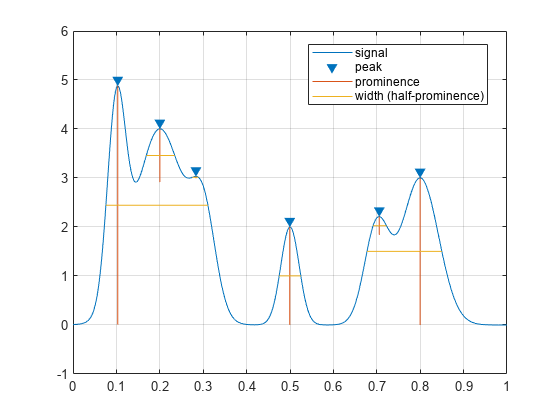
Use findpeaks to locate and plot the peaks that have a prominence of at least 4.
findpeaks(PeakSig,x,'MinPeakProminence',4,'Annotate','extents')
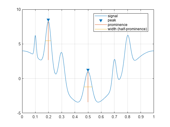
The highest and lowest peaks are the only ones that satisfy the condition.
Display the prominences and the widths at half prominence of all the peaks.
[pks,locs,widths,proms] = findpeaks(PeakSig,x);
widths
widths = 1×6

    0.0154    0.0431    0.0377    0.0625    0.0274    0.0409
proms = 1×6

    2.6816    5.5773    3.1448    4.4171    2.9191    3.6363
Find Peaks with Minimum Separation
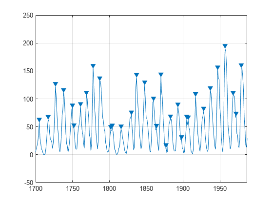
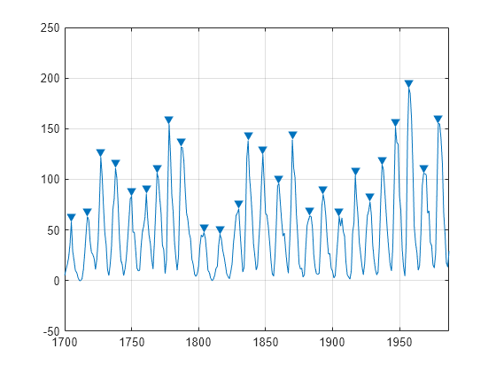
Sunspots are a cyclic phenomenon. Their number is known to peak roughly every 11 years.
Load the file sunspot.dat, which contains the average number of sunspots observed every year from 1700 to 1987. Find and plot the maxima.
load sunspot.dat

year = sunspot(:,1);
avSpots = sunspot(:,2);

findpeaks(avSpots,year)
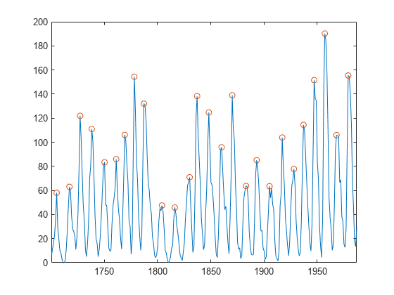
Improve your estimate of the cycle duration by ignoring peaks that are very close to each other. Find and plot the peaks again, but now restrict the acceptable peak-to-peak separations to values greater than six years.
findpeaks(avSpots,year,'MinPeakDistance',6)
Use the peak locations returned by findpeaks to compute the mean interval between maxima.
[pks,locs] = findpeaks(avSpots,year,'MinPeakDistance',6);

meanCycle = mean(diff(locs))
Create a datetime array using the year data. Assume the sunspots were counted every year on March 20th, close to the vernal equinox. Find the peak sunspot years. Use the years function to specify the minimum peak separation as a duration.
ty = datetime(year,3,20);

[pk,lk] = findpeaks(avSpots,ty,'MinPeakDistance',years(6));

plot(ty,avSpots,lk,pk,'o')
Compute the mean sunspot cycle using datetime functionality.
dttmCycle = years(mean(diff(lk)))
Create a timetable with the data. Specify the time variable in years. Plot the data. Show the last five entries of the timetable.
TT = timetable(years(year),avSpots);
plot(TT.Time,TT.Variables)
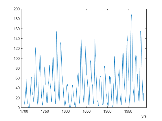
entries = TT(end-4:end,:)
entries=5×1 timetable
      Time      avSpots
    ________    _______

    1983 yrs     66.6
    1984 yrs     45.9
    1985 yrs     17.9
    1986 yrs     13.4
    1987 yrs     29.3
Constrain Peak Features
Load an audio signal sampled at 7418 Hz. Select 200 samples.
load mtlb
select = mtlb(1001:1200);
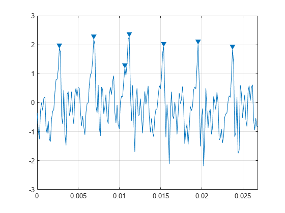
Find the peaks that are separated by at least 5 ms.
To apply this constraint, findpeaks chooses the tallest peak in the signal and eliminates all peaks within 5 ms of it. The function then repeats the procedure for the tallest remaining peak and iterates until it runs out of peaks to consider.
findpeaks(select,Fs,'MinPeakDistance',0.005)
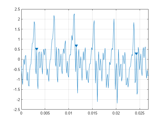
Find the peaks that have an amplitude of at least 1 V.
findpeaks(select,Fs,'MinPeakHeight',1)
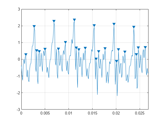
Find the peaks that are at least 1 V higher than their neighboring samples.
findpeaks(select,Fs,'Threshold',1)
Find the peaks that drop at least 1 V on either side before the signal attains a higher value.
findpeaks(select,Fs,'MinPeakProminence',1)
Peaks of Saturated Signal
Sensors can return clipped readings if the data are larger than a given saturation point. You can choose to disregard these peaks as meaningless or incorporate them to your analysis.
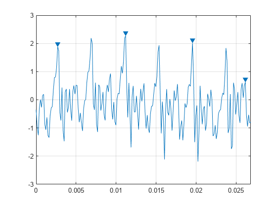
Generate a signal that consists of a product of trigonometric functions of frequencies 5 Hz and 3 Hz embedded in white Gaussian noise of variance 0.1². The signal is sampled for one second at a rate of 100 Hz. Reset the random number generator for reproducible results.
rng default

fs = 1e2;
t = 0:1/fs:1-1/fs;

s = sin(2*pi*5*t).*sin(2*pi*3*t)+randn(size(t))/10;
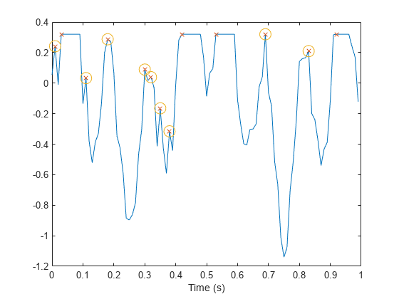
Simulate a saturated measurement by truncating every reading that is greater than a specified bound of 0.32. Plot the saturated signal.
bnd = 0.32;
s(s>bnd) = bnd;

plot(t,s)
xlabel('Time (s)')

Locate the peaks of the signal. findpeaks reports only the rising edge of each flat peak.
[pk,lc] = findpeaks(s,t);

hold on
plot(lc,pk,'x')

Use the 'Threshold' name-value pair to exclude the flat peaks. Require a minimum amplitude difference of 10-4 between a peak and its neighbors.
[pkt,lct] = findpeaks(s,t,'Threshold',1e-4);

plot(lct,pkt,'o','MarkerSize',12)
Determine Peak Widths
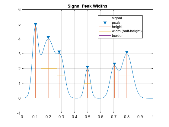
Create a signal that consists of a sum of bell curves. Specify the location, height, and width of each curve.
x = linspace(0,1,1000);

Pos = [1 2 3 5 7 8]/10;
Hgt = [4 4 2 2 2 3];
Wdt = [3 8 4 3 4 6]/100;

for n = 1:length(Pos)
    Gauss(n,:) =  Hgt(n)*exp(-((x - Pos(n))/Wdt(n)).^2);
end

PeakSig = sum(Gauss);
Plot the individual curves and their sum.
plot(x,Gauss,'--',x,PeakSig)
grid
Measure the widths of the peaks using the half prominence as reference.
findpeaks(PeakSig,x,'Annotate','extents')
Measure the widths again, this time using the half height as reference.
findpeaks(PeakSig,x,'Annotate','extents','WidthReference','halfheight')
title('Signal Peak Widths')
Input Arguments
collapse all
data — Input data
vector
Input data, specified as a vector. data must
be real and must have at least three elements.
Data Types: double | single
x — Locations
vector | datetime array
Locations, specified as a vector or a datetime array. x must
increase monotonically and have the same length as data.
If x is omitted, then the indices of data are
used as locations.
Data Types: double | single | datetime
Fs — Sample rate
positive scalar
Sample rate, specified as a positive scalar. The sample rate
is the number of samples per unit time. If the unit of time is seconds,
the sample rate has units of hertz.
Data Types: double | single
Name-Value Arguments
Specify optional pairs of arguments as
Name1=Value1,...,NameN=ValueN, where Name is
the argument name and Value is the corresponding value.
Name-value arguments must appear after other arguments, but the order of the
pairs does not matter.
Before R2021a, use commas to separate each name and value, and enclose
Name in quotes.
Example: 'SortStr','descend','NPeaks',3 finds
the three tallest peaks of the signal.
NPeaks — Maximum number of peaks
positive integer scalar
Maximum number of peaks to return, specified as a positive integer scalar.
findpeaks operates from the first element of the
input data and terminates when the number of peaks reaches the value of
'NPeaks'.
Data Types: double | single
SortStr — Peak sorting
'none' (default) | 'ascend' | 'descend'
Peak sorting, specified as one of these values:
-
'none'returns the peaks in the
order in which they occur in the input data. -
'ascend'returns the peaks in ascending
or increasing order, from the smallest to the largest value. -
'descend'returns the peaks in
descending order, from the largest to the smallest value.
MinPeakHeight — Minimum peak height
-Inf (default) | real scalar
Minimum peak height, specified as a real scalar. Use this argument to have
findpeaks return only those peaks higher than
'MinPeakHeight'. Specifying a minimum peak height
can reduce processing time.
Data Types: double | single
MinPeakProminence — Minimum peak prominence
0 (default) | real scalar
Minimum peak prominence, specified as a real scalar. Use this argument to have
findpeaks return only those peaks that have a
relative importance of at least 'MinPeakProminence'.
For more information, see Prominence.
Data Types: double | single
Threshold — Minimum height difference
0 (default) | nonnegative real scalar
Minimum height difference between a peak and its neighbors, specified as a nonnegative real
scalar. Use this argument to have findpeaks return
only those peaks that exceed their immediate neighboring values by at
least the value of 'Threshold'.
Data Types: double | single
MinPeakDistance — Minimum peak separation
0 (default) | positive real scalar
Minimum peak separation, specified as a positive real scalar. When you specify a value for
'MinPeakDistance', the algorithm chooses the
tallest peak in the signal and ignores all peaks within
'MinPeakDistance' of it. The function then
repeats the procedure for the tallest remaining peak and iterates until
it runs out of peaks to consider.
-
If you specify a location vector,
x,
then'MinPeakDistance'must be expressed
in terms ofx. If
xis adatetime
array, then specify'MinPeakDistance'as
adurationscalar or as a numeric scalar
expressed in days. -
If you specify a sample rate,
Fs,
then'MinPeakDistance'must be expressed
in units of time. -
If you specify neither
xnor
Fs, then
'MinPeakDistance'must be expressed
in units of samples.
Use this argument to have findpeaks
ignore small peaks that occur in the neighborhood of a larger
peak.
Data Types: double | single | duration
WidthReference — Reference height for width measurements
'halfprom' (default) | 'halfheight'
Reference height for width measurements, specified as either 'halfprom' or
'halfheight'. findpeaks
estimates the width of a peak as the distance between the points where
the descending signal intercepts a horizontal reference line. The height
of the line is selected using the criterion specified in
'WidthReference':
-
'halfprom'positions the reference line
beneath the peak at a vertical distance equal to half the
peak prominence. See Prominence for more
information. -
'halfheight'positions the reference
line at one-half the peak height. The line is truncated if
any of its intercept points lie beyond the borders of the
peaks selected by setting
'MinPeakHeight',
'MinPeakProminence', and
'Threshold'. The border between peaks
is defined by the horizontal position of the lowest valley
between them. Peaks with height less than zero are
discarded.
The locations of the intercept points are computed by
linear interpolation.
MinPeakWidth — Minimum peak width
0 (default) | positive real scalar
Minimum peak width, specified as a positive real scalar. Use this argument to select only
those peaks that have widths of at least
'MinPeakWidth'.
-
If you specify a location vector,
x,
then'MinPeakWidth'must be expressed in
terms ofx. Ifx
is adatetimearray, then specify
'MinPeakWidth'as a
durationscalar or as a numeric
scalar expressed in days. -
If you specify a sample rate,
Fs,
then'MinPeakWidth'must be expressed in
units of time. -
If you specify neither
xnor
Fs, then
'MinPeakWidth'must be expressed in
units of samples.
Data Types: double | single | duration
MaxPeakWidth — Maximum peak width
Inf (default) | positive real scalar
Maximum peak width, specified as a positive real scalar. Use this argument to select only
those peaks that have widths of at most
'MaxPeakWidth'.
-
If you specify a location vector,
x,
then'MaxPeakWidth'must be expressed in
terms ofx. Ifx
is adatetimearray, then specify
'MaxPeakWidth'as a
durationscalar or as a numeric
scalar expressed in days. -
If you specify a sample rate,
Fs,
then'MaxPeakWidth'must be expressed in
units of time. -
If you specify neither
xnor
Fs, then
'MaxPeakWidth'must be expressed in
units of samples.
Data Types: double | single | duration
Annotate — Plot style
'peaks' (default) | 'extents'
Plot style, specified as one of these values:
-
'peaks'plots the signal and annotates
the location and value of every peak. -
'extents'plots the signal and
annotates the location, value, width, and prominence of every peak.
This argument is ignored if you call findpeaks with
output arguments.
Output Arguments
collapse all
pks — Local maxima
vector
Local maxima, returned as a vector of signal values. If there
are no local maxima, then pks is empty.
locs — Peak locations
vector
Peak locations, returned as a vector.
-
If you specify a location vector,
x,
thenlocscontains the values ofxat
the peak indices. -
If you specify a sample rate,
Fs, then
locsis a numeric vector of time
instants with a time difference of 1/Fs
between consecutive samples. -
If you specify neither
xnorFs,
thenlocsis a vector of integer indices.
w — Peak widths
vector
Peak widths, returned as a vector of real numbers. The width
of each peak is computed as the distance between the points to the
left and right of the peak where the signal intercepts a reference
line whose height is specified by WidthReference.
The points themselves are found by linear interpolation.
-
If you specify a location vector,
x,
then the widths are expressed in terms ofx. -
If you specify a sample rate,
Fs,
then the widths are expressed in units of time. -
If you specify neither
xnorFs,
then the widths are expressed in units of samples.
p — Peak prominences
vector
Peak prominences, returned as a vector of real numbers. The
prominence of a peak is the minimum vertical distance that the signal
must descend on either side of the peak before either climbing back
to a level higher than the peak or reaching an endpoint. See Prominence for more information.
More About
collapse all
Prominence
The prominence of a peak
measures how much the peak stands out due to its intrinsic height
and its location relative to other peaks. A low isolated peak can
be more prominent than one that is higher but is an otherwise unremarkable
member of a tall range.
To measure the prominence of a peak:
-
Place a marker on the peak.
-
Extend a horizontal line from the peak to the left
and right until the line does one of the following:-
Crosses the signal because there is a higher peak
-
Reaches the left or right end of the signal
-
-
Find the minimum of the signal in each of the two
intervals defined in Step 2. This point is either
a valley or one of the signal endpoints. -
The higher of the two interval minima specifies the
reference level. The height of the peak above this level is its prominence.
findpeaks makes no assumption about the behavior of the signal beyond its
endpoints, whatever their height. As a result, Steps 2 and 4 disregard signal
behavior beyond endpoints, which often affects the value of the reference level.
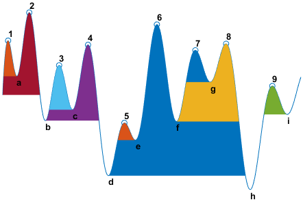
Consider for example the peaks of this signal:

| Peak Number | Left Interval Lies Between Peak and | Right Interval Lies Between Peak and | Lowest Point on the Left Interval | Lowest Point on the Right Interval | Reference Level (Highest Minimum) |
|---|---|---|---|---|---|
| 1 | Left end | Crossing due to peak 2 | Left endpoint | a | a |
| 2 | Left end | Right end | Left endpoint | h | Left endpoint |
| 3 | Crossing due to peak 2 | Crossing due to peak 4 | b | c | c |
| 4 | Crossing due to peak 2 | Crossing due to peak 6 | b | d | b |
| 5 | Crossing due to peak 4 | Crossing due to peak 6 | d | e | e |
| 6 | Crossing due to peak 2 | Right end | d | h | d |
| 7 | Crossing due to peak 6 | Crossing due to peak 8 | f | g | g |
| 8 | Crossing due to peak 6 | Right end | f | h | f |
| 9 | Crossing due to peak 8 | Crossing due to right endpoint | h | i | i |
Extended Capabilities
C/C++ Code Generation
Generate C and C++ code using MATLAB® Coder™.
GPU Arrays
Accelerate code by running on a graphics processing unit (GPU) using Parallel Computing Toolbox™.
This function fully supports GPU arrays. For more information, see Run MATLAB Functions on a GPU (Parallel Computing Toolbox).
Version History
Introduced in R2007b
Main Content
PeakFinderConfiguration
Compute and display the largest calculated peak values on the scope
display
Since R2022a
Description
Use the PeakFinderConfiguration object to compute and display
peaks in the scope. The scope computes and displays peaks for only the portion of the input
signal that is currently on display in the scope.
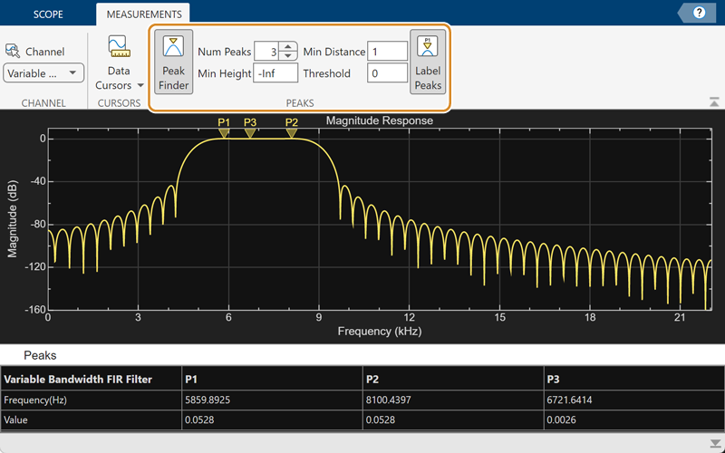
You can specify the number of peaks you want the scope to display, the minimum height
above which you want the scope to detect peaks, the minimum distance between peaks, and label
the peaks. You can control the peak finder settings from the scope toolstrip or from the
command line. The algorithm defines a peak as a local maximum with lower values present on
either side of the peak. It does not consider end points as peaks. For more information on the
algorithm, see the findpeaks function.
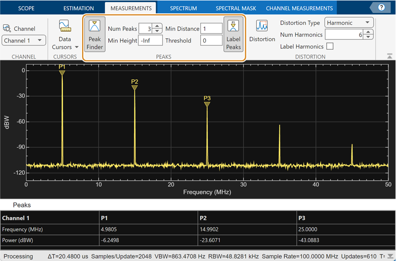
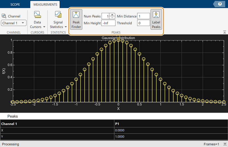
To modify the peak finder settings in the scope interface, click the
Measurements tab and enable Peak Finder. Once you
enable the Peak Finder, an arrow appears on the plot at each maxima and a
Peaks panel appears at the bottom of the scope window.
The SpectrumAnalyzerConfiguration
object supports the PeakFinderConfiguration object in the command
line.
Spectrum Analyzer Toolstrip
Time Scope Toolstrip

Array Plot Toolstrip
Dynamic Filter Visualizer
Toolstrip
Creation
Syntax
Description
example
pkfinder = PeakFinderConfiguration() creates a peak finder
configuration object.
Properties
expand all
All properties are tunable.
MinHeight — Level above which scope detects peaks
-Inf (default) | real scalar value
Level above which the scope detects peaks, specified as a real scalar.
Scope Window Use
On the Measurements tab, select Peak Finder. In the
peak finder settings, specify a real scalar in the
Min Height
box.
Data Types: double
NumPeaks — Maximum number of peaks to show
3 (default) | positive integer less than 100
Maximum number of peaks to show, specified as a positive integer less than 100.
Scope Window Use
On the Measurements tab, select Peak
Finder. In the peak finder settings, specify a positive integer less
than 100 in the Num Peaks box.
Data Types: double
MinDistance — Minimum number of samples between adjacent peaks
1 (default) | positive integer
Minimum number of samples between adjacent peaks, specified as a positive integer.
Scope Window Use
On the Measurements tab, select Peak
Finder. In the peak finder settings, specify a positive integer in
the Min Distance box.
Data Types: double
Threshold — Minimum difference in height of peak and its neighboring samples
0 (default) | nonnegative scalar
Minimum difference in the height of the peak and its neighboring samples, specified as a
nonnegative scalar.
Scope Window Use
On the Measurements tab, select Peak
Finder. In the peak finder settings, specify a nonnegative scalar in
the Threshold box.
Data Types: double
LabelPeaks — Label found peaks
false (default) | true
Label found peaks, specified as true or false. The scope displays the labels (P1, P2, …) above the arrows in the plot.
Scope Window Use
On the Measurements tab, select Peak
Finder. In the peak finder settings, select Label Peaks.
Data Types: logical
LabelFormat — Coordinates to display
"x + y" (default) | "x" | "y"
Coordinates to display next to the calculated peak value, specified as "x", "y", or "x + y".
Data Types: char | string
Enabled — Enable peak finder measurements
false (default) | true
Enable peak finder measurements, specified as true or
false. Set this property to
true to enable the peak finder
measurements.
Scope Window Use
On the Measurements tab, select Peak Finder.
Data Types: logical
Examples
collapse all
Enable Peak Finder Programmatically in a Time Scope Object
Create a sine wave and view it in the Time Scope. Enable the peak finder programmatically.
Initialization
Create the input sine wave using the sin function. Create a timescope MATLAB® object to display the signal. Set the TimeSpan property to 1 second.
f = 100;
fs = 1000;
swv = sin(2.*pi.*f.*(0:1/fs:1-1/fs)).';
scope = timescope(SampleRate=fs,...
    TimeSpanSource="property", ...
    TimeSpan=1);
Peaks
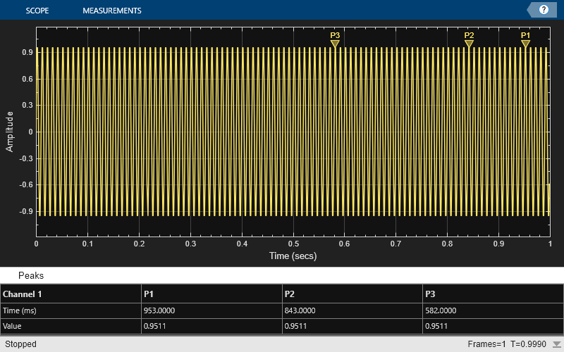
Enable the peak finder and label the peaks. Set the scope to show three peaks and label them.
scope.PeakFinder.Enabled = true;
scope.PeakFinder.LabelPeaks = true;
scope(swv)
release(scope)
Obtain Measurements Data Programmatically for spectrumAnalyzer object
Compute and display the power spectrum of a noisy sinusoidal input signal using the spectrumAnalyzer MATLAB® object. Measure the peaks, cursor placements, adjacent channel power ratio, and distortion values in the spectrum by enabling these properties:
-
PeakFinder -
CursorMeasurements -
ChannelMeasurements -
DistortionMeasurements
Initialization
The input sine wave has two frequencies: 1000 Hz and 5000 Hz. Create two dsp.SineWave System objects to generate these two frequencies. Create a spectrumAnalyzer object to compute and display the power spectrum.
Fs = 44100;
Sineobject1 = dsp.SineWave(SamplesPerFrame=1024,PhaseOffset=10,...
    SampleRate=Fs,Frequency=1000);
Sineobject2 = dsp.SineWave(SamplesPerFrame=1024,...
    SampleRate=Fs,Frequency=5000);
SA = spectrumAnalyzer(SampleRate=Fs,SpectrumType="power",...
    PlotAsTwoSidedSpectrum=false,ChannelNames={'Power spectrum of the input'},...
    YLimits=[-120 40],ShowLegend=true);
Enable Measurements Data
To obtain the measurements, set the Enabled property to true.
SA.CursorMeasurements.Enabled = true;
SA.ChannelMeasurements.Enabled = true;
SA.PeakFinder.Enabled = true;
SA.DistortionMeasurements.Enabled = true;
Use getMeasurementsData
Stream in the noisy sine wave input signal and estimate the power spectrum of the signal using the spectrumAnalyzer object. Measure the characteristics of the spectrum. Use the getMeasurementsData function to obtain these measurements programmatically. The isNewDataReady function returns true when there is new spectrum data. Store the measured data in the variable data.
data = [];
for Iter = 1:1000
    Sinewave1 = Sineobject1();
    Sinewave2 = Sineobject2();
    Input = Sinewave1 + Sinewave2;
    NoisyInput = Input + 0.001*randn(1024,1);
    SA(NoisyInput);
     if SA.isNewDataReady
        data = [data;getMeasurementsData(SA)];
     end
end
The panes at the bottom of the scope window display the measurements that you have enabled. The values in these panes match the values in the last time step of the data variable. You can access the individual fields of data to obtain the various measurements programmatically.
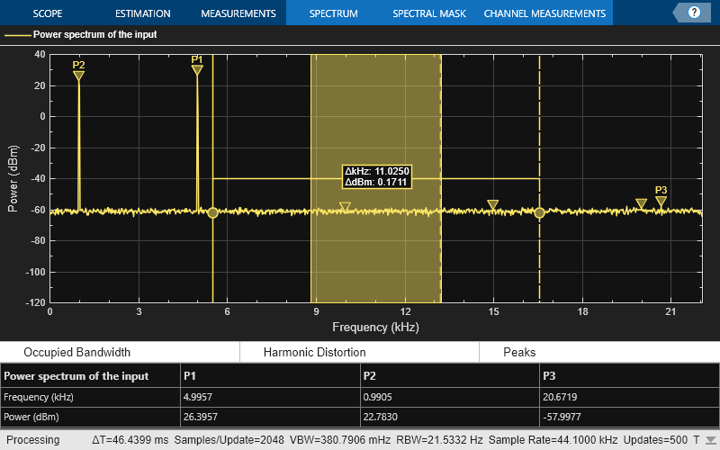
Compare Peak Values
Use the PeakFinder property to obtain peak values. Verify that the peak values in the last time step of data match the values in the spectrum analyzer plot.
peakvalues = data.PeakFinder(end).Value
peakvalues = 3×1

   26.3957
   22.7830
  -57.9977
frequencieskHz = data.PeakFinder(end).Frequency/1000
frequencieskHz = 3×1

    4.9957
    0.9905
   20.6719
Version History
Introduced in R2022a
expand all
R2023a: Support for Spectrum Analyzer block
The SpectrumAnalyzerConfiguration
object now supports the PeakFinderConfiguration object. The
PeakFinderConfiguration object enables you to obtain and modify the peak
finder measurements of the Spectrum Analyzer block programmatically from the
command line.

Всем привет!
На этот раз столкнулся с другой задачей — есть множество однотипных графиков (около 10 тысяч). Все они похожи на прикрепленный файл с нектороым смещением по оси Х.
Нужно написать код, который бы на всех графиках находил вершины пиков (количесто воодится вручную от 1 до 12) и далее делал бы необходимый анализ — амплитуда, сигма и тд.
Но вот что-то никак не могу придумать простой способ разыскать пики. Сильно давить шум на графиках нельзя, во всяком случае пока.
Подскажите, как это лучше сделать?
Вот кусок моего кода — он находит точное положение центров, но для этого надо мышкой тыкать по пикам.
| Matlab M | ||
|
Найдите локальные максимумы
Синтаксис
Описание
пример
pks = findpeaks(data)data. Локальный пик является выборкой данных, которая или больше, чем ее две соседних выборки или равна Inf. Non-Inf конечные точки сигнала исключены. Если пик является плоским, функция возвращает только точку с самым низким индексом.
пример
[ дополнительно возвращает индексы, в которых происходит peaks.pks,locs] = findpeaks(data)
пример
[ дополнительно возвращает ширины peaks как векторный pks,locs,w,p]
= findpeaks(data)w и выдающиеся положения peaks как векторный p.
пример
[___] = findpeaks( задает data,x)x как вектор местоположения и возвращает любой из выходных аргументов от предыдущих синтаксисов. locs и w описываются в терминах x.
пример
[___] = findpeaks( задает частоту дискретизации, data,Fs)Fs, из данных. Первая выборка data принят, чтобы быть взятыми в начальный момент времени. locs и w преобразованы в единицы измерения времени.
пример
[___] = findpeaks(___, задает аргументы пары «имя-значение» использования опций в дополнение к любому из входных параметров в предыдущих синтаксисах.Name,Value)
пример
findpeaks(___) без выходных аргументов строит сигнал и накладывает пиковые значения.
Примеры
свернуть все
Найдите Peaks в векторе
Задайте вектор с тремя peaks и постройте его.
data = [25 8 15 5 6 10 10 3 1 20 7];
plot(data)

Найдите локальные максимумы. Peaks выводится в порядке вхождения. Первая выборка не включена несмотря на то, чтобы быть максимумом. Для плоского пика функция возвращает только точку с самым низким индексом.
Используйте findpeaks без выходных аргументов, чтобы отобразить peaks.

Найдите Peaks и их местоположения
Создайте сигнал, который состоит из суммы кривых нормального распределения. Задайте местоположение, высоту и ширину каждой кривой.
x = linspace(0,1,1000);

Pos = [1 2 3 5 7 8]/10;
Hgt = [3 4 4 2 2 3];
Wdt = [2 6 3 3 4 6]/100;

for n = 1:length(Pos)
    Gauss(n,:) = Hgt(n)*exp(-((x - Pos(n))/Wdt(n)).^2);
end

PeakSig = sum(Gauss);
Постройте отдельные кривые и их сумму.
plot(x,Gauss,'--',x,PeakSig)

Используйте findpeaks с настройками по умолчанию, чтобы найти peaks сигнала и их местоположений.
[pks,locs] = findpeaks(PeakSig,x);
Постройте peaks с помощью findpeaks и пометьте их.
findpeaks(PeakSig,x)

text(locs+.02,pks,num2str((1:numel(pks))'))

Сортировка peaks от самого высокого до самого короткого.
[psor,lsor] = findpeaks(PeakSig,x,'SortStr','descend');

findpeaks(PeakSig,x)

text(lsor+.02,psor,num2str((1:numel(psor))'))

Пиковые выдающиеся положения
Создайте сигнал, который состоит из суммы кривых нормального распределения, едущих на полном периоде косинуса. Задайте местоположение, высоту и ширину каждой кривой.
x = linspace(0,1,1000);

base = 4*cos(2*pi*x);

Pos = [1 2 3 5 7 8]/10;
Hgt = [3 7 5 5 4 5];
Wdt = [1 3 3 4 2 3]/100;

for n = 1:length(Pos)
    Gauss(n,:) =  Hgt(n)*exp(-((x - Pos(n))/Wdt(n)).^2);
end

PeakSig = sum(Gauss)+base;
Постройте отдельные кривые и их сумму.
plot(x,Gauss,'--',x,PeakSig,x,base)

Используйте findpeaks определять местоположение и строить peaks, который имеет выдающееся положение по крайней мере 4.
findpeaks(PeakSig,x,'MinPeakProminence',4,'Annotate','extents')

Самый высокий и самый низкий peaks является единственными единицами, которые удовлетворяют условию.
Отобразите выдающиеся положения и ширины в половине выдающегося положения всего peaks.
[pks,locs,widths,proms] = findpeaks(PeakSig,x);
widths
widths = 1×6

    0.0154    0.0431    0.0377    0.0625    0.0274    0.0409
proms = 1×6

    2.6816    5.5773    3.1448    4.4171    2.9191    3.6363
Найдите Peaks с минимальным разделением
Солнечные пятна являются циклическим явлением. Их номер, как известно, достигает максимума примерно каждые 11 лет.
Загрузите файл sunspot.dat, который содержит среднее количество солнечных пятен, наблюдаемых каждый год от 1 700 до 1987. Найдите и постройте максимумы.
load sunspot.dat

year = sunspot(:,1);
avSpots = sunspot(:,2);

findpeaks(avSpots,year)

Улучшите свою оценку длительности цикла путем игнорирования peaks, который является очень друг близко к другу. Найдите и постройте peaks снова, но теперь ограничьте приемлемые разделения от пика к пику значениями, больше, чем шесть лет.
findpeaks(avSpots,year,'MinPeakDistance',6)

Используйте пиковые местоположения, возвращенные findpeaks вычислить средний интервал между максимумами.
[pks,locs] = findpeaks(avSpots,year,'MinPeakDistance',6);

meanCycle = mean(diff(locs))
Создайте datetime массив с помощью данных года. Примите, что солнечные пятна считались каждый год 20-го марта, близко к весеннему равноденствию. Найдите пиковые годы солнечного пятна. Используйте years функция, чтобы задать минимальное пиковое разделение как duration.
ty = datetime(year,3,20);

[pk,lk] = findpeaks(avSpots,ty,'MinPeakDistance',years(6));

plot(ty,avSpots,lk,pk,'o')

Вычислите средний цикл солнечной активности с помощью datetime функциональность.
dttmCycle = years(mean(diff(lk)))
Создайте расписание с данными. Задайте переменную времени в годах. Отобразите данные на графике. Покажите последние пять записей расписания.
TT = timetable(years(year),avSpots);
plot(TT.Time,TT.Variables)

entries = TT(end-4:end,:)
entries=5×1 timetable
      Time      avSpots
    ________    _______

    1983 yrs     66.6
    1984 yrs     45.9
    1985 yrs     17.9
    1986 yrs     13.4
    1987 yrs     29.3
Ограничьте пиковые функции
Загрузите звуковой сигнал, произведенный на уровне 7 418 Гц. Выберите 200 выборок.
load mtlb
select = mtlb(1001:1200);
Найдите peaks, который разделяется по крайней мере на 5 мс.
Применять это ограничение, findpeaks выбирает самый высокий пик в сигнале и устраняет весь peaks в 5 мс из него. Функция затем повторяет процедуру для самого высокого остающегося пика и выполняет итерации, пока это не исчерпывает peaks, чтобы рассмотреть.
findpeaks(select,Fs,'MinPeakDistance',0.005)

Найдите peaks, который имеет амплитуду по крайней мере 1 В.
findpeaks(select,Fs,'MinPeakHeight',1)

Найдите peaks, который на по крайней мере 1 В выше, чем их соседние выборки.
findpeaks(select,Fs,'Threshold',1)

Найдите peaks, который понижается по крайней мере на 1 В с обеих сторон, прежде чем сигнал достигает более высокого значения.
findpeaks(select,Fs,'MinPeakProminence',1)

Peaks влажного сигнала
Датчики могут возвратить отсеченные показания, если данные больше, чем данная точка насыщения. Можно принять решение игнорировать этот peaks как бессмысленный или включить их к анализу.
Сгенерируйте сигнал, который состоит из продукта тригонометрических функций частот 5 Гц и 3 Гц, встроенные в белый Гауссов шум отклонения 0,1 ². Сигнал производится в течение одной секунды на уровне 100 Гц. Сбросьте генератор случайных чисел для восстанавливаемых результатов.
rng default

fs = 1e2;
t = 0:1/fs:1-1/fs;

s = sin(2*pi*5*t).*sin(2*pi*3*t)+randn(size(t))/10;
Симулируйте влажное измерение путем усечения каждого чтения, которое больше заданного, связанного 0,32. Постройте влажный сигнал.
bnd = 0.32;
s(s>bnd) = bnd;

plot(t,s)
xlabel('Time (s)')

Найдите peaks сигнала. findpeaks отчеты только возрастающее ребро каждого плоского пика.
[pk,lc] = findpeaks(s,t);

hold on
plot(lc,pk,'x')

Используйте 'Threshold' пара «имя-значение», чтобы исключить плоский peaks. Потребуйте минимального амплитудного различия 10-4 между пиком и его соседями.
[pkt,lct] = findpeaks(s,t,'Threshold',1e-4);

plot(lct,pkt,'o','MarkerSize',12)

Определите пиковые ширины
Создайте сигнал, который состоит из суммы кривых нормального распределения. Задайте местоположение, высоту и ширину каждой кривой.
x = linspace(0,1,1000);

Pos = [1 2 3 5 7 8]/10;
Hgt = [4 4 2 2 2 3];
Wdt = [3 8 4 3 4 6]/100;

for n = 1:length(Pos)
    Gauss(n,:) =  Hgt(n)*exp(-((x - Pos(n))/Wdt(n)).^2);
end

PeakSig = sum(Gauss);
Постройте отдельные кривые и их сумму.
plot(x,Gauss,'--',x,PeakSig)
grid

Измерьте ширины peaks с помощью половины выдающегося положения в качестве ссылки.
findpeaks(PeakSig,x,'Annotate','extents')

Измерьте ширины снова, на этот раз с помощью половины высоты в качестве ссылки.
findpeaks(PeakSig,x,'Annotate','extents','WidthReference','halfheight')
title('Signal Peak Widths')

Входные параметры
свернуть все
data — Входные данные
вектор
Входные данные в виде вектора. data должно быть действительным и должен иметь по крайней мере три элемента.
Типы данных: double | single
x — Местоположения
вектор | datetime массив
Местоположения в виде вектора или datetime массив. x должен увеличиться монотонно и иметь ту же длину как data. Если x не использован, затем индексы data используются в качестве местоположений.
Типы данных: double | single | datetime
Fs — Частота дискретизации
положительная скалярная величина
Частота дискретизации в виде положительной скалярной величины. Частота дискретизации является количеством отсчетов в единицу времени. Если модуль времени является секундами, частота дискретизации имеет модули герц.
Типы данных: double | single
Аргументы name-value
Задайте дополнительные разделенные запятой пары Name,Value аргументы. Name имя аргумента и Value соответствующее значение. Name должен появиться в кавычках. Вы можете задать несколько аргументов в виде пар имен и значений в любом порядке, например: Name1, Value1, ..., NameN, ValueN.
Пример: 'SortStr','descend','NPeaks',3 находит три самых высоких peaks сигнала.
NPeaks — Максимальное количество peaks
положительный целочисленный скаляр
Максимальное количество peaks, чтобы возвратиться в виде разделенной запятой пары, состоящей из 'NPeaks' и положительный целочисленный скаляр. findpeaks действует от первого элемента входных данных и завершает работу, когда количество peaks достигает значения 'NPeaks'.
Типы данных: double | single
SortStr — Пиковая сортировка
'none' (значение по умолчанию) | 'ascend' | 'descend'
Пиковая сортировка в виде разделенной запятой пары, состоящей из 'SortStr' и одно из этих значений:
-
'none'возвращает peaks в порядке, в котором они происходят во входных данных. -
'ascend'возвращает peaks в возрастании или увеличении порядка, от самого маленького до самого большого значения. -
'descend'возвращает peaks в порядке убывания, от самого большого до наименьшего значения.
MinPeakHeight — Минимальная пиковая высота
-Inf (значение по умолчанию) | действительный скаляр
Минимальная пиковая высота в виде разделенной запятой пары, состоящей из 'MinPeakHeight' и действительный скаляр. Используйте этот аргумент, чтобы иметь findpeaks возвратите только тот peaks выше, чем 'MinPeakHeight'. Определение минимальной пиковой высоты может уменьшать время вычислений.
Типы данных: double | single
MinPeakProminence — Минимальное пиковое выдающееся положение
0 (значений по умолчанию) | действительный скаляр
Минимальное пиковое выдающееся положение в виде разделенной запятой пары, состоящей из 'MinPeakProminence' и действительный скаляр. Используйте этот аргумент, чтобы иметь findpeaks возвратите только тот peaks, который имеет относительную важность, по крайней мере, 'MinPeakProminence'. Для получения дополнительной информации смотрите Выдающееся положение.
Типы данных: double | single
Threshold — Минимальная разность высот
0 (значений по умолчанию) | неотрицательный действительный скаляр
Минимальная разность высот между пиком и его соседями в виде разделенной запятой пары, состоящей из 'Threshold' и неотрицательный действительный скаляр. Используйте этот аргумент, чтобы иметь findpeaks возвратите только тот peaks, который превышает их мгновенные соседние значения, по крайней мере, значением 'Threshold'.
Типы данных: double | single
MinPeakDistance — Минимальное пиковое разделение
0 (значений по умолчанию) | положительный действительный скаляр
Минимальное пиковое разделение в виде разделенной запятой пары, состоящей из 'MinPeakDistance' и положительный действительный скаляр. Когда вы задаете значение для 'MinPeakDistance', алгоритм выбирает самый высокий пик в сигнале и игнорирует весь peaks в 'MinPeakDistance' из него. Функция затем повторяет процедуру для самого высокого остающегося пика и выполняет итерации, пока это не исчерпывает peaks, чтобы рассмотреть.
-
Если вы задаете вектор местоположения,
x, затем'MinPeakDistance'должен быть описан в терминахx. Еслиxdatetimeмассив, затем задайте'MinPeakDistance'какdurationскаляр или в виде числа описывается в днях. -
Если вы задаете частоту дискретизации,
Fs, затем'MinPeakDistance'должен быть описан в модулях времени. -
Если вы не задаете никакой
xниFs, затем'MinPeakDistance'должен быть описан в модулях выборок.
Используйте этот аргумент, чтобы иметь findpeaks проигнорируйте маленький peaks, который происходит в окружении более крупного пика.
Типы данных: double | single | duration
WidthReference — Ссылочная высота для измерений ширины
'halfprom' (значение по умолчанию) | 'halfheight'
Ссылочная высота для измерений ширины в виде разделенной запятой пары, состоящей из 'WidthReference' и любой 'halfprom' или 'halfheight'. findpeaks оценивает ширину пика как расстояние между точками, где убывающий сигнал прерывает горизонтальную ссылочную линию. Высота линии выбрана с помощью критерия, заданного в 'WidthReference':
-
'halfprom'располагает ссылочную линию ниже пика на вертикальном расстоянии, равном половине пикового выдающегося положения. Смотрите Выдающееся положение для получения дополнительной информации. -
'halfheight'располагает ссылочную линию в половине пиковой высоты. Линия является усеченной, если какая-либо из ее точек пересечения лежит за пределами границ peaks, выбранного установкой'MinPeakHeight','MinPeakProminence', и'Threshold'. Граница между peaks задана горизонтальным положением самого низкого оврага между ними. Peaks с высотой меньше, чем нуль отбрасывается.
Местоположения точек пересечения вычисляются линейной интерполяцией.
MinPeakWidth — Минимальная пиковая ширина
0 (значений по умолчанию) | положительный действительный скаляр
Минимальная пиковая ширина в виде разделенной запятой пары, состоящей из 'MinPeakWidth' и положительный действительный скаляр. Используйте этот аргумент, чтобы выбрать только тот peaks, который имеет ширины, по крайней мере, 'MinPeakWidth'.
-
Если вы задаете вектор местоположения,
x, затем'MinPeakWidth'должен быть описан в терминахx. Еслиxdatetimeмассив, затем задайте'MinPeakWidth'какdurationскаляр или в виде числа описывается в днях. -
Если вы задаете частоту дискретизации,
Fs, затем'MinPeakWidth'должен быть описан в модулях времени. -
Если вы не задаете никакой
xниFs, затем'MinPeakWidth'должен быть описан в модулях выборок.
Типы данных: double | single | duration
MaxPeakWidth — Максимальная пиковая ширина
Inf (значение по умолчанию) | положительный действительный скаляр
Максимальная пиковая ширина в виде разделенной запятой пары, состоящей из 'MaxPeakWidth' и положительный действительный скаляр. Используйте этот аргумент, чтобы выбрать только тот peaks, который имеет ширины в большей части 'MaxPeakWidth'.
-
Если вы задаете вектор местоположения,
x, затем'MaxPeakWidth'должен быть описан в терминахx. Еслиxdatetimeмассив, затем задайте'MaxPeakWidth'какdurationскаляр или в виде числа описывается в днях. -
Если вы задаете частоту дискретизации,
Fs, затем'MaxPeakWidth'должен быть описан в модулях времени. -
Если вы не задаете никакой
xниFs, затем'MaxPeakWidth'должен быть описан в модулях выборок.
Типы данных: double | single | duration
Annotate — Стиль графика
'peaks' (значение по умолчанию) | 'extents'
Стиль графика в виде разделенной запятой пары, состоящей из 'Annotate' и одно из этих значений:
-
'peaks'строит сигнал и аннотирует местоположение и значение каждого пика. -
'extents'строит сигнал и аннотирует местоположение, значение, ширину и выдающееся положение каждого пика.
Этот аргумент проигнорирован, если вы вызываете findpeaks с выходными аргументами.
Выходные аргументы
свернуть все
pks — Локальные максимумы
вектор
Локальные максимумы, возвращенные как вектор из значений сигналов. Если нет никаких локальных максимумов, то pks isempty.
locs — Пиковые местоположения
вектор
Пиковые местоположения, возвращенные как вектор.
-
Если вы задаете вектор местоположения,
x, затемlocsсодержит значенияxв пиковых индексах. -
Если вы задаете частоту дискретизации,
Fs, затемlocsчисловой вектор моментов времени с разницей во времени 1/Fsмежду последовательными выборками. -
Если вы не задаете никакой
xниFs, затемlocsвектор из целочисленных индексов.
w — Пиковые ширины
вектор
Пиковые ширины, возвращенные как вектор из вещественных чисел. Ширина каждого пика вычисляется как расстояние между точками налево и правом пика, где сигнал прерывает ссылочную линию, высота которой задана WidthReference. Сами точки найдены линейной интерполяцией.
-
Если вы задаете вектор местоположения,
x, затем ширины описываются в терминахx. -
Если вы задаете частоту дискретизации,
Fs, затем ширины описываются в модулях времени. -
Если вы не задаете никакой
xниFs, затем ширины описываются в модулях выборок.
p — Пиковые выдающиеся положения
вектор
Пиковые выдающиеся положения, возвращенные как вектор из вещественных чисел. Выдающееся положение пика является минимальным вертикальным расстоянием, что сигнал должен убывать по обе стороны от пика прежде или поднимающийся назад на уровень выше, чем пик или достигающий конечной точки. Смотрите Выдающееся положение для получения дополнительной информации.
Больше о
свернуть все
Выдающееся положение
Выдающееся положение пика измеряется, насколько пик выделяется из-за его внутренней высоты и его местоположения относительно другого peaks. Низкий изолированный пик может быть более видным, чем тот, который выше, но является в противном случае обыкновенным членом высокой области значений.
Измерять выдающееся положение пика:
-
Поместите маркер в пик.
-
Расширьте горизонтальную линию от пика налево и прямо пока линия не выполнит одно из следующих действий:
-
Пересекает сигнал, потому что существует более высокий пик
-
Достигает левого или правого конца сигнала
-
-
Найдите минимум сигнала в каждом из этих двух интервалов заданным на Шаге 2. Эта точка является или оврагом или одной из конечных точек сигнала.
-
Выше двух минимумов интервала задает контрольный уровень. Высота пика выше этого уровня является своим выдающимся положением.
findpeaks не делает предположения о поведении сигнала вне его конечных точек, безотносительно их высоты. Это отражается на Шагах 2 и 4 и часто влияет на значение контрольного уровня. Рассмотрите, например, peaks этого сигнала:
| Пиковый номер | Оставленный интервал находится между пиком и | Правильный интервал находится между пиком и | Самая низкая точка на левом интервале | Самая низкая точка на правильном интервале | Контрольный уровень (самый высокий минимум) |
|---|---|---|---|---|---|
| 1 | Оставленный конец | Пересечение должного достигнуть максимума 2 | Оставленная конечная точка | a | a |
| 2 | Оставленный конец | Правильный конец | Оставленная конечная точка | h | Оставленная конечная точка |
| 3 | Пересечение должного достигнуть максимума 2 | Пересечение должного достигнуть максимума 4 | b | c | c |
| 4 | Пересечение должного достигнуть максимума 2 | Пересечение должного достигнуть максимума 6 | b | d | b |
| 5 | Пересечение должного достигнуть максимума 4 | Пересечение должного достигнуть максимума 6 | d | e | e |
| 6 | Пересечение должного достигнуть максимума 2 | Правильный конец | d | h | d |
| 7 | Пересечение должного достигнуть максимума 6 | Пересечение должного достигнуть максимума 8 | f | g | g |
| 8 | Пересечение должного достигнуть максимума 6 | Правильный конец | f | h | f |
| 9 | Пересечение должного достигнуть максимума 8 | Пересечение из-за правильной конечной точки | h | i | i |
Расширенные возможности
Генерация кода C/C++
Генерация кода C и C++ с помощью MATLAB® Coder™.
Представленный в R2007b
Ничего лучшего, чем поиск пиков в массиве в голову не приходит. Строгое чередование положительных и отрицательных пиков облегчает задачу.
Т.е. алгоритм примерно такой.
Выбираем значения двух порогов: положительного и отрицательного. Ищем максимум пока сигнал больше отрицательного порога. Найденный максимум и есть пик, а индекс в массиве — его позиция. Ждем превышения положительного порога и ищем очередной положительный пик. Пороги подбираются так, чтобы быть выше шума: колебания около нуля. Их значения могут быть ясны исходя из природы сигнала (минимально возможная величина пика), либо можно попытаться их вычислить статистически (найти среднеквадратическое отклонение шума и установить порог в значение, например 3 СКО).
Боюсь, что готовой функции в библиотеках не будет. Однако реализация такого алгоритма тривиальна. К сожалению, с Python мало знаком, поэтому приведу возможную реализацию на C++ (думаю, что проблем с пониманием возникнуть не должно):
typedef double sample_type;
struct Peak {
    sample_type magnitude;
    std::size_t pos;
};
std::vector<Peak> peaks(const std::vector<sample_type> &sig) {
    static sample_type threshold_lo = -0.05;
    static sample_type threshold_hi = 0.05;
    std::vector<Peak> ret_peaks;
    std::vector<sample_type>::size_type isample = 0;
    while (1) {
        while ((isample < sig.size()) && (sig[isample] < threshold_hi)) {
            ++isample;
        }
        if (isample >= sig.size())
            break;
        ret_peaks.push_back(Peak(sig[isample], isample));
        while ((isample < sig.size()) && (sig[isample] > threshold_lo)) {
            if (sig[isample] > ret_peaks.back().magnitude) {
                ret_peaks.back().magnitude = sig[isample];
                ret_peaks.back().pos = isample;
            }
            ++isample;
        }
        if (isample >= sig.size())
            break;
    }
    return ret_peaks;
}
Можно также использовать корреляцию (для ее вычисления должна быть готовая функция в scipy). Но, на мой взгляд, в данном случае это более сложный подход. О корреляции можно также почитать здесь