Как составить модель dcf - Исправление недочетов и поиск решений вместе с Examum.ru

КУРС

ФИНАНСОВОЕ МОДЕЛИРОВАНИЕ

Научитесь строить финансовые модели любой сложности для оценки компаний из различных отраслей, а также для прогнозирования их денежных потоков.

В серии статей мы рассмотрим пошаговое построение базовой модели DCF. Для начала необходимо определить экономическую сущность модели дисконтирования денежных потоков (от англ. Discounted cash flow).

Дисконтирование денежных потоков является одним из наиболее важных и используемых методов для оценки стоимости компании.

Основная цель данной методики заключается в определении объема денежных средств, которые инвестор может получить при инвестировании в компанию, акцию или какой-либо другой актив. Если величина денежных потоков будет превышать вложенные средства, то компания/актив будет являться привлекательным для инвестиций. Отработать на практике изложенные в статье материалы можно на нашем открытом онлайн-курсе «Построение DCF-модели».

В качестве примера проводить анализ будем на финансовой отчетности крупной публичной компании Wallmart. Все финансовые показатели можно найти на сайте анализируемой компании или на других внешних источниках (Yahoo Finance, Google Finance, Bloomberg и др.)

Расчет Enterprise Value

Стоимость предприятия (Enterprise Value) – это примерная стоимость компании, которую бы заплатил потенциальный покупатель.

Как посчитать Enterprise Value? Данный показатель состоит из суммы рыночной капитализации, неконтролирующих долей и чистого долга, который определяется как разность общего долга и денежных средств.

Enterprise Value = Market Capitalization + (Total Debt – Cash) + Minority Interest

Рыночная капитализация — это цена одной акции, умноженная на общее количество акций. Стоит отметить, что в расчете необходимо использовать только разводненные акции, то есть то количество, которое включает в себя опционы, выпущенные для менеджеров и ключевых сотрудников компании. Такие опционы со временем конвертируются в акции. Это один из видов компенсаций, который получают сотрудники помимо заработной платы.

Так как мы хотим получить справедливую стоимость акций, нам необходимо рассмотреть именно разводненное количество акций, то есть мы должны учесть тот эффект, что через некоторое время кто-то будет владеть этими акциями. Количество разводненных акций (diluted) мы можем найти в консолидированном отчете о финансовых результатах компании.

Что такое финансовый долг?

Это долг, который:

имеет процентную нагрузку;
был выдан кредитными организациями.

Финансовый долг включает в себя банковские кредиты, финансовый лизинг, облигации, и другие кредиты, выданные кредитными организациями, фондами, лизинговыми компаниями.

Чтобы посчитать общий долг, мы вновь обращаемся к бухгалтерскому балансу. В показатель Total Debt входят:

Краткосрочные займы;
Долг с погашением в течение одного года;
Финансовый лизинг с погашением в течение одного года;
Долгосрочный кредит;
Долгосрочный финансовый лизинг

Показатель денежных средств тоже определяем из баланса, в разделе оборотных активов. Для чего мы вычитаем Cash? Потенциальные покупатели компании хотят приобрести активы, которые могут генерировать деньги. Другими словами, их не интересует покупка денежных средств. Компания, у которой на балансе нет ничего кроме денег, не имеет ценности. Вы просто заплатите деньги за получение доступа к банковскому счету. Следовательно, можно сделать вывод, что чем больше у компании показатель Cash, тем меньше ее стоимость.

Также для расчета Enterprise Value необходим показатель «Неконтролирующие доли» (Total Minority Interest / Non-controlling interest), который располагается в балансе в разделе Капитал. Неконтролирующие доли – это та часть чистых активов в дочерних предприятиях компании, которыми она не владеет.

Таким образом, Enterprise Value – это более точный показатель стоимость компании, чем рыночная капитализация, которая оценивает только капитал, то есть только чистые активы, принадлежащие акционерам этой компании.

Расчет стоимости капитала

Средневзвешенная стоимость капитала (WACC, Weighted average cost of capital) – это средняя процентная ставка по всем источникам финансирования компании, которая используется для дисконтирования ожидаемых денежных потоков.

Как рассчитать данный показатель? У компании имеется два вида капитала: собственный и заемный. Зная суммы собственного и долгового капиталов и их веса, мы можем получить средневзвешенную стоимость капитала, очистив при этом долговой капитал от налогов.

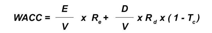
E/V – доля акционерного капитала в общем капитале. Если акции котируются на бирже, то V– рыночная стоимость акционерного капитала. Если не котируются, то V– балансовая стоимость акционерного капитала. E/Vможно рассчитать, как Market Capitalization / Total Debt.

Re — стоимость акционерного капитала (рассчитывается с помощью модели CAPM);

D/V — доля долгового капитала в общем капитале. Обычно используется балансовая стоимость акционерного капитала.

Rd — стоимость долгового капитала. При возможности необходимо использовать рыночную стоимость долга. В отчетности можно рассчитать, как Interest Expenses/ Total Debt. Ставка является приблизительной, так как для точного значения необходимо анализировать весь кредитный портфель, что обычно затруднительно найти в открытых источниках.

1 – Тс — эффект налогового щита. Суть эффекта заключается в том, что чем выше проценты по кредитам, тем ниже сумма налогов. Чем выше налоговая ставка, тем ниже стоимость долгового капитала. Иными словами, процентные платежи уменьшают налоговую базу, то есть уменьшают прибыль до налогов. Для определения Tax Rate в отчете о финансовых результатах необходимо размер начисленных налогов разделить на доналоговую прибыль (EBT) по каждому анализируемому периоду.

Стоимость акционерного капитала (Cost of Equity) – средняя ожидаемая доходность по акциям публичной компании. Чтобы рассчитать этот показатель, необходимо обратиться к модели CAPM (Capital Asset Pricing Model).

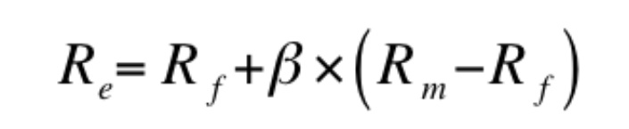
формула расчета стоимости акционерного капитала

Re — cost of equity, стоимость акционерного капитала;
Rf — risk-free rate, безрисковая ставка;
Rm — market risk, средняя доходность фондового рынка;
Rm – Rf — рыночная премия;
b — коэффициент чувствительности изменения цены по отношению к рынку. b>1 – стоимость акций компании растет быстрее рынка, b<1 – стоимость акций компании растет медленнее рынка.

За безрисковую ставку можем принять процентные ставки государственных ценных бумаг в соответствии со страной, компанию которой мы оцениваем. Если в прогнозе рассматривается диапазон до 5 лет, то необходимо использовать ставку доходности пятилетней государственной бумаги. Например, при анализе российской компании используют 5-10 летние бумаги ОФЗ, для компаний из США – 10 летняя доходность Treasuries, в Европе – долгосрочные доходности по облигациям Германии или Франции.

Рыночный риск – это ожидаемая доходность по рынку, на котором торгуются акции анализируемой компании. Рыночная премия – это дополнительная доходность, которую получает инвестор за то, что он инвестировал денежные средства не в безрисковые активы.

Коэффициент Бета рассчитывается с помощью регрессии, однако обычно его публикуют на разных финансовых агрегаторах (Yahoo Finance, Google Finance).

Таким образом, WACC является ставкой дисконтирования, которая используется для определения текущей стоимости прогнозируемых будущих денежных потоков.

В следующих частях статьи мы перейдем непосредственно к дисконтированию денежных потоков, конструированию сценариев и прогнозам необходимых показателей.

Блог SF Education

Финансы

Что такое Enterprise Value?

Статья доступна в аудиоверсии Enterprise Value, как один из показателей, имеющих непосредственное отношение к оценке и стоимости бизнеса, является одной из ключевых метрик в…

Пошаговое построение модели DCF. Часть 3: расчет ∆NWC, FCFF, Terminal Value, Total Enterprise Value

Завершаем серию статей, где мы рассказываем о пошаговом построении базовой модели дисконтированных денежных потоков. Если хотите узнать еще больше о финансовом моделировании, то записывайтесь…

Источник

Бесплатное руководство как построить DCF модель в Excel.

Модель DCF — это особый вид финансового моделирования, используемый для оценки стоимости бизнеса. DCF расшифровывается как Discounted Cash Flow, поэтому модель DCF — это просто прогноз свободного денежного потока компании без учета дисконтирования до сегодняшней стоимости, которая называется чистой текущей стоимостью (NPV). Это учебное руководство по модели DCF шаг за шагом научит вас основам.

Несмотря на простоту концепции, для каждого из упомянутых выше компонентов требуется довольно много технических знаний, поэтому давайте разберем каждый из них более подробно. Основным структурным элементом модели DCF является финансовая модель из трех отчетов, которая связывает финансовые отчеты воедино. Это учебное руководство по DCF-модели проведет вас через все шаги, которые необходимо знать, чтобы построить такую модель самостоятельно.

Что такое неориентированный свободный денежный поток?

Денежный поток — это просто денежные средства, генерируемые компанией, которые могут быть распределены среди инвесторов или реинвестированы в компанию. Нелеверизованный свободный денежный поток (также называемый свободным денежным потоком фирмы) — это денежные средства, которые доступны как долговым, так и долевым инвесторам. Чтобы узнать больше, прочтите наше руководство по расчету нелеверизованного свободного денежного потока и как его рассчитать.

Денежный поток используется потому, что он отражает экономическую ценность, в то время как бухгалтерские показатели, такие как чистый доход, этого не делают. Компания может иметь положительный чистый доход, но отрицательный денежный поток, что подрывает экономическую эффективность бизнеса. Денежные средства — это то, что инвесторы действительно ценят в конце дня, а не бухгалтерская прибыль.

Почему денежный поток дисконтируется?

Денежный поток, генерируемый бизнесом, дисконтируется к определенному моменту времени (отсюда и название модели дисконтированного денежного потока), обычно к текущей дате. Причина дисконтирования денежных потоков сводится к нескольким причинам, которые в основном сводятся к стоимости возможностей и риску, в соответствии с теорией временной стоимости денег. Временная стоимость денег предполагает, что деньги в настоящем стоят больше, чем деньги в будущем, потому что деньги в настоящем можно инвестировать и тем самым заработать больше денег.

Средневзвешенная стоимость капитала компании (WACC) представляет собой требуемую норму прибыли, ожидаемую инвесторами. Поэтому его можно также рассматривать как альтернативную стоимость компании, то есть если она не может найти более высокую норму прибыли в другом месте, ей следует выкупить свои собственные акции.

Если компания получает доходность выше стоимости капитала (пороговой ставки), то она «создает стоимость». Если они получают доходность ниже стоимости капитала, то они «разрушают стоимость».

Требуемая инвесторами норма прибыли (как обсуждалось выше) обычно связана с риском инвестиций (с использованием модели ценообразования капитальных активов). Поэтому, чем рискованнее инвестиции, тем выше требуемая норма прибыли и выше стоимость капитала.

Чем дальше отстоят денежные потоки, тем они рискованнее и, следовательно, их необходимо дисконтировать дальше.

Как построить прогноз денежных потоков в модели DCF

Это обширная тема, и за прогнозированием показателей бизнеса стоит целое искусство. Проще говоря, работа финансового аналитика заключается в том, чтобы сделать максимально обоснованный прогноз о том, как каждый из факторов, влияющих на бизнес, повлияет на его результаты в будущем. Подробнее об этом читайте в нашем руководстве по допущениям и прогнозированию.

Как правило, прогноз для модели DCF составляет приблизительно пять лет, за исключением ресурсных отраслей или отраслей с длительным сроком эксплуатации, таких как горнодобывающая, нефтегазовая и инфраструктурная, где для построения долгосрочного прогноза «срока службы ресурсов» могут использоваться инженерные отчеты.

1. Прогнозирование выручки

Существует несколько способов построения прогноза выручки, но в целом они делятся на две основные категории: на основе роста и на основе драйверов.

Прогноз на основе роста более прост и имеет смысл для стабильных, зрелых компаний, где можно использовать базовый темп роста за год. Для многих моделей DCF этого вполне достаточно.

Прогноз на основе драйверов является более детальным и сложным для разработки. Он требует разбивки выручки на различные факторы, такие как цена, объем, продукция, клиенты, доля рынка и внешние факторы. Регрессионный анализ часто используется как часть прогноза на основе драйверов для определения взаимосвязи между базовыми драйверами и ростом выручки.

2. Прогнозирование расходов

Построение прогноза расходов может быть очень подробным и детализированным процессом, или же это может быть простое сравнение по годам.

Наиболее детальный подход называется «нулевым бюджетом» и предполагает построение расходов с нуля без учета того, что было потрачено в прошлом году. Как правило, каждый отдел компании просят обосновать все имеющиеся у него расходы, исходя из вида деятельности.

Этот подход часто используется в условиях сокращения расходов или при введении финансового контроля. Его практическое применение возможно только внутри компании менеджерами, а не сторонними лицами, такими как инвестиционные банкиры или аналитики по исследованию акций.

3. Прогнозирование капитальных активов и изменений в оборотном капитале

Когда большая часть отчета о прибылях и убытках составлена, наступает время прогнозирования капитальных активов. Основные средства часто являются самой крупной статьей баланса и капитальные затраты (CapEx), а также амортизация должны быть смоделированы в отдельном графике.

Наиболее детальный подход заключается в создании отдельного графика в модели DCF для каждого из основных капитальных активов, а затем их объединение в общий график. Каждый график капитальных активов будет включать несколько строк: начальный баланс, капитальные вложения, амортизация, выбытие и конечный баланс.

Изменение оборотного капитала, включающее дебиторскую, кредиторскую задолженность и запасы, должно быть рассчитано и добавлено или вычтено в зависимости от их влияния на денежные средства.

4. Прогнозирование структуры капитала

Построение этого раздела во многом зависит от того, какой тип DCF-модели вы строите. Наиболее распространенный подход заключается в том, чтобы просто сохранить текущую структуру капитала компании, не допуская никаких серьезных изменений, кроме тех, которые известны, например, срок погашения долга.

Поскольку мы используем неливелированный свободный денежный поток, этот раздел на самом деле не так важен для модели DCF. Однако он важен, если вы смотрите на ситуацию с точки зрения инвестора или аналитика по исследованию рынка акций. Инвестиционные банкиры обычно фокусируются на стоимости предприятия, поскольку она более актуальна для сделок M&A, когда покупается или продается вся компания.

5. Терминальная стоимость

Терминальная стоимость является очень важной частью модели DCF. Часто она составляет более 50% чистой приведенной стоимости бизнеса, особенно если прогнозный период составляет пять лет или меньше. Существует два способа расчета терминальной стоимости: подход с использованием вечных темпов роста и подход с использованием коэффициента выхода.

Метод постоянного темпа роста предполагает, что денежный поток, генерируемый в конце прогнозного периода, вечно растет с постоянной скоростью. Так, например, денежный поток бизнеса составляет $10 млн и вечно растет на 2%, а стоимость капитала составляет 15%. Терминальная стоимость составляет $10 млн / (15% — 2%) = $77 млн.

При подходе с использованием коэффициента выхода предполагается, что бизнес будет продан за ту сумму, которую за него заплатит «разумный покупатель». Обычно это означает мультипликатор EV/EBITDA на уровне или близко к текущей торговой стоимости сопоставимых компаний. Как видно из примера ниже, если EBITDA предприятия составляет $6,3 млн, а аналогичные компании торгуются по цене 8x, то терминальная стоимость составляет $6,3 млн x 8 = $50 млн. Эта стоимость затем дисконтируется к настоящему времени, чтобы получить NPV терминальной стоимости.

6. Сроки денежных потоков

Важно обратить пристальное внимание на сроки денежных потоков в модели DCF, поскольку не все временные периоды обязательно равны. Часто в начале модели есть «промежуточный период», когда получена только часть денежного потока за год. Кроме того, отток денежных средств (осуществление фактических инвестиций), как правило, приходится на промежуточный период времени до получения «заглушки».

Функции XNPV и XIRR — это простые способы очень точно определить время денежных потоков при построении модели DCF. Лучшая практика — всегда использовать их вместо обычных функций Excel NPV и IRR.

7. DCF Стоимость предприятия

При построении модели DCF с использованием нелевереджированного свободного денежного потока NPV, которую вы получаете, всегда является стоимостью предприятия (EV) бизнеса. Это то, что вам нужно, если вы хотите оценить весь бизнес или сравнить его с другими компаниями без учета их структуры капитала (т.е. сравнение «яблоко к яблоку»). В большинстве инвестиционно-банковских сделок основное внимание уделяется стоимости предприятия.

8. DCF Стоимость акционерного капитала

Если вы ищете стоимость собственного капитала компании, вы берете чистую приведенную стоимость (NPV) нелевереджированного свободного денежного потока и корректируете ее на денежные средства и эквиваленты, долг и долю меньшинства. Это даст вам стоимость собственного капитала, которую вы можете разделить на количество акций и получить цену акций. Такой подход более характерен для институциональных инвесторов или аналитиков, занимающихся исследованием акций, которые смотрят через призму покупки или продажи акций.

Анализ чувствительности в модели DCF

После завершения модели DCF (т.е. получения NPV бизнеса) наступает время для анализа чувствительности, чтобы определить, в каком диапазоне стоимости может оказаться бизнес при изменении различных факторов или допущений в модели.

Для проведения такого анализа аналитик использует два основных инструмента Excel: таблицы данных и поиск целей. Связав NPV бизнеса с ячейками, которые влияют на основные допущения, можно увидеть, как меняется стоимость при различных исходных данных.

Дополнительные ресурсы:

Мы надеемся, что вам понравилось читать статью Finansistem про DCF модель. Finansistem поможет каждому стать финансовым аналитиком мирового класса. Приведенные ниже ресурсы будут полезны для дальнейшего развития вашего финансового образования:

Выигрышное мышление успешного трейдера
Вопросы и ответы на собеседовании по инвестиционно-банковской деятельности
Лучшие инвестиционные банки
Руководство по финансовому моделированию
Виды финансовых моделей

Источник

What is a DCF Model?

The Discounted Cash Flow Model, or “DCF Model”, is a type of financial model that values a company by forecasting its cash flows and discounting them to arrive at a current, present value.

DCFs are widely used in both academia and in practice.

Valuing companies using a DCF model is considered a core skill for investment bankers, private equity, equity research and “buy side” investors.

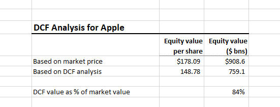
This DCF analysis suggests that Apple might be overvalued (or that our assumptions are wrong!)

A DCF model estimates a company’s intrinsic value (the value based on a company’s ability to generate cash flows) and is often presented in comparison to the company’s market value.

For example, Apple has a market capitalization of approximately $909 billion. Is that market price justified based on the company’s fundamentals and expected future performance (i.e. its intrinsic value)? That is exactly what a DCF seeks to answer.

In contrast with market-based valuation like a comparable company analysis, the idea behind the DCF model is that the value of a company is not a function of arbitrary supply and demand for that company’s stock. Instead, the value of a company is a function of a company’s ability to generate cash flow in the future for its shareholders.

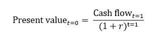
DCF Model Basics: Present Value Formula

The DCF approach requires that we forecast a company’s future cash flows and discount them to the present in order to arrive at a present value for the company. That present value is the amount investors should be willing to pay (the company’s value). We can express this formulaically as the follwoing (we denote the discount rate as r):

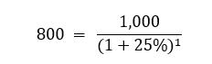
So, let’s say you decide you’re willing to pay $800 for the below. We can solve this as:

If I make the same proposition but instead of only promising $1,000 next year, say I promise $1,000 for the next 5 years.The math gets only slightly more complicated:

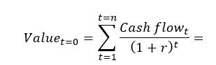
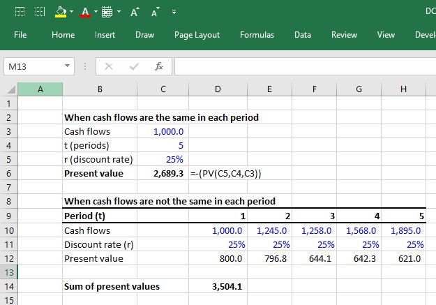
In Excel, you can calculate this using the PV function (see below). However, if cash flows are different each year, you will have to discount each cash flow separately:

Learn More → Investment Banking Primer

DCF Model in Excel – Sample Template Download

Use the form below to download our sample DCF model template:

How to Build a DCF Model: 6-Step Framework

The premise of the DCF model is that the value of a business is purely a function of its future cash flows. Thus, the first challenge in building a DCF model is to define and calculate the cash flows that a business generates. There are two common approaches to calculating the cash flows that a business generates.

Unlevered DCF approach
Forecast and discount the operating cash flows. Then, when you have a present value, just add any non-operating assets such as cash and subtract any financing-related liabilities such as debt.
Levered DCF approach
Forecast and discount the cash flows that remain available to equity shareholders after cash flows to all non-equity claims (i.e. debt) have been removed.

Both should theoretically lead to the same value at the end (though in practice it’s actually pretty hard to get them to be exactly equal). The unlevered DCF approach is the most common and is thus the focus of this guide. This approach involves 6 steps:

Step 1. Forecasting unlevered free cash flows

Step 1 is to forecast the cash flows a company generates from its core operations after accounting for all operating expenses and investments.
These cash flows are called “unlevered free cash flows.”

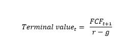
Step 2. Calculating the terminal value

You can’t keep forecasting cash flows forever. At some point, you must make some high-level assumptions about cash flows beyond the final explicit forecast year by estimating a lump-sum value of the business past the explicit forecast period.
That lump sum is called the “terminal value.”

Step 3. Discounting the cash flows to the present at the weighted average cost of capital

The discount rate that reflects the riskiness of the unlevered free cash flows is called the weighted average cost of capital.
Because unlevered free cash flows represent all operating cash flows, these cash flows “belong” to both the company’s lenders and owners.
As such, the risks of both providers of capital (i.e. debt vs. equity) need to be accounted for using appropriate capital structure weights (hence the term “weighted average” cost of capital).
Once discounted, the present value of all unlevered free cash flows is called the enterprise value.

Step 4. Add the value of non-operating assets to the present value of unlevered free cash flows

If a company has any non-operating assets such as cash or has some investments just sitting on the balance sheet, we must add them to the present value of unlevered free cash flows.
For example, if we calculate that the present value of Apple’s unlevered free cash flows is $700 billion, but then we discover that Apple also has $200 billion in cash just sitting around, we should add this cash.

Step 5. Subtract debt and other non-equity claims

The ultimate goal of the DCF is to get at what belongs to the equity owners (equity value).
Therefore if a company has any lenders (or any other non-equity claims against the business), we need to subtract this from the present value.
What’s left over belongs to the equity owners.
In our example, if Apple had $50 billion in debt obligations at the valuation date, the equity value would be calculated as:
- $700 billion (enterprise value) + $200 billion (non-operating assets) – $50 (debt) = $850 billion
Often, the non-operating assets and debt claims are added together as one term called net debt (debt and other non-equity claims – non-operating assets).
You’ll often see the equation: enterprise value – net debt = equity value. The equity value that the DCF calculates is comparable to the market capitalization (the market’s perception of the equity value).

Step 6. Divide the equity value by the shares outstanding

The equity value tells us what the total value to owners is. But what is the value of each share? In order to calculate this, we divide the equity value by the company’s diluted shares outstanding.

Calculating Unlevered Free Cash Flows (FCF)

Here is the formula for unlevered free cash flow:

FCF = EBIT x (1- tax rate) + D&A + NWC – Capital expenditures

EBIT = Earnings before interest and taxes. This represents a company’s GAAP-based operating profit.
Tax rate = The tax rate the company is expected to face. When forecasting taxes, we usually use a company’s historical effective tax rate.
D&A = Depreciation and amortization.
NWC = Annual changes in net working capital. Increases in NWC are cash outflows while decreases are cash inflows.
Capital expenditures represent cash investments the company must make in order to sustain the forecasted growth of the business. If you don’t factor in the cost of required reinvestment into the business, you will overstate the value of the company by giving it credit for EBIT growth without accounting for the investments required to achieve it.

FCFs are ideally driven from a 3-statement model

Forecasting all these line items should ideally come from a 3-statement model because all of the components of unlevered free cash flows are interrelated: Changes in EBIT assumptions impact capex, NWC, and D&A. Without a 3-statement model that dynamically links all these components together, it is difficult to ensure that the changes in assumptions of one component correctly impact the other components.

Because this takes more work and more time, finance professionals often do preliminary analyses using a quick, back-of-the-envelope DCF model and only build a full DCF model driven by a 3-statement model when the stakes are high, such as when an investment banking deal goes “live” or when a private equity firm is in the later stages of the investment process.

The 2-stage DCF model

The 3-statement models that support a DCF are usually annual models that forecast about 5-10 years into the future. However, when valuing businesses, we usually assume they are a going concern. In other words, the assumption is that they will continue to operate forever.

That means that the 3-statement model only takes us so far. We also have to forecast the present value of all future unlevered free cash flows after the explicit forecast period. This is called the 2-stage DCF model. The first stage is to forecast the unlevered free cash flows explicitly (and ideally from a 3-statement model). The second stage is the total of all cash flows after stage 1. This typically entails making some assumptions about the company reaching mature growth. The present value of the stage 2 cash flows is called the terminal value.

Prefer video? To watch a free video lesson on how to build a DCF, click here.

Calculating the terminal value

In a DCF, the terminal value (TV) represents the value the company will generate from all the expected free cash flows after the explicit forecast period. Imagine that we calculate the following unlevered free cash flows for Apple:

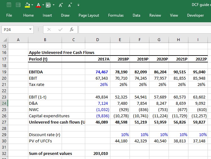
Apple is expected to generate cash flows beyond 2022, but we cannot project FCFs forever (with any degree of accuracy). So how do we estimate the value of Apple beyond 2022? There are two common approaches:

Growth in Perpetuity
Exit EBITDA Multiple Method

The growth in perpetuity approach

The growth in perpetuity approach assumes Apple’s UFCFs will grow at some constant growth rate assumption from 2022 to … forever. The formula for calculating the present value of a cash flow growing at a constant growth rate in perpetuity is called the “Growth in perpetuity formula”:

If we assume that after 2022, Apple’s UFCFs will grow at a constant 4% rate into perpetuity and will face a weighted average cost of capital of 10% in perpetuity, the terminal value (which is the present value of all Apple’s future cash flows beyond 2022) is calculated as:

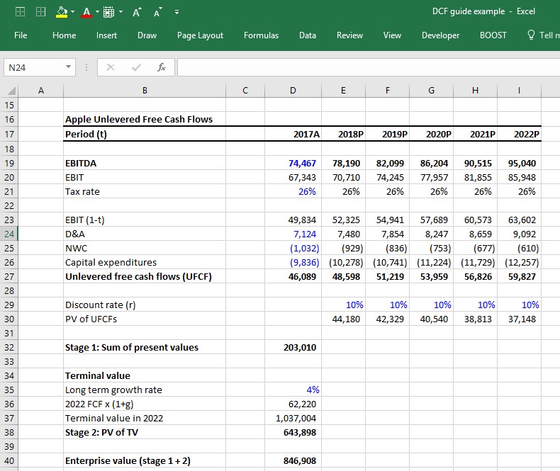
At this point, notice that we have finally calculated enterprise value as simply the sum of the stage 1 present value of UFCFs + the present value of the stage 2 terminal value.

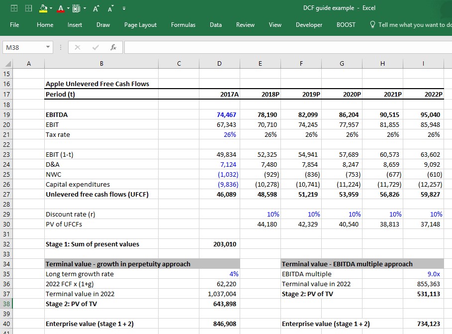
Exit EBITDA Multiple Method

The growth in perpetuity approach forces us to guess the long-term growth rate of a company. The result of the analysis is very sensitive to this assumption. A way around having to guess a company’s long term growth rate is to guess the EBITDA multiple the company will be valued at the last year of the stage 1 forecast.

A common way to do this is to look at the current EV/EBITDA multiple the company is trading at (or the average EV/EBITDA multiple of the company’s peer group) and assume the company will be valued at that same multiple in the future. For example, if Apple is currently valued at 9.0x its last twelve months (LTM) EBITDA, we can assume that in 2022 it will be valued at 9.0x its 2022 EBITDA.

Growth in perpetuity vs. exit EBITDA multiple method

Investment bankers and private equity professionals tend to be more comfortable with the EBITDA multiple approach because it infuses market reality into the DCF. A private equity professional building a DCF will likely try to figure out what he/she can sell the company for 5 years down the road, so this arguably provides a valuation via an EBITDA multiple.

However, this approach suffers from a significant conceptual problem: It incorporates current market valuations within the DCF, which arguably defeats the whole purpose of the DCF. Making matters worse is the fact that the terminal value often represents a significant pecentage of the value contribution in a DCF, so the assumptions that go into calculating the terminal value are all the more important.

Getting to enterprise value: Discounting the cash flows by the WACC

Up to now, we’ve been assuming a 10% discount rate for Apple, but how is that actually quantified? Quantifying the discount rate, which in this case is the weighted average cost of capital (WACC), is a critical field of study in corporate finance. You can spend an entire college semester learning about it. We’ve written a complete guide to WACC here, but below are the basic elements for how it is typically calculated:

The WACC formula

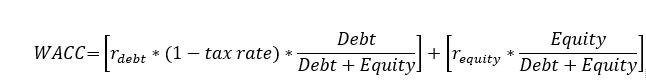
Where:

Debt = market value of debt
Equity = market value of equity
r_debt= cost of debt
r_equity= cost of equity

Getting to equity value: Adding the value of non-operating assets

Many companies have assets not directly tied to operations. Assets such as cash obviously increase the value of the company (i.e. a company whose operations are worth $1 billion but also has $100 million in cash is worth $1.1 billion). But up to now, the value is not accounted for in the unlevered free cash flow calculation. Therefore, these assets need to be added to the value. The most common non-operating assets include:

Cash
Marketable securities
Equity investments

Below is Apple’s 2016 year-end balance sheet. The non-operating assets are its cash and equivalents, short-term marketable securities and long-term marketable securities. As you can see, they represent a significant portion of the company’s balance sheet.

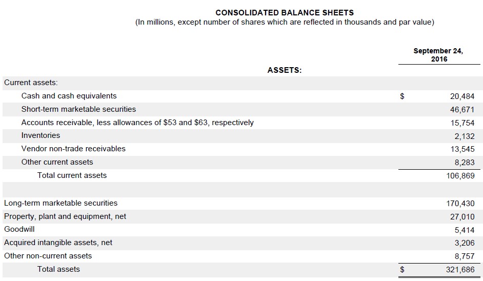
Unlike operating assets such as PP&E, inventory and intangible assets, the carrying value of non-operating assets on the balance sheet is usually fairly close to their actual value. That’s because they are mostly comprised of cash and liquid investments that companies generally can mark up to fair value. That’s not always the case (equity investments are a notable exception), but it’s typically safe to simply use the latest balance sheet values of non-operating assets as the actual market values.

Getting to equity value: Subtracting debt and other non-equity claims

At this point, we need to identify and subtract all non-equity claims on the business in order to arrive at how much of the company value actually belongs to equity owners. The most common non-equity claims you’ll encounter are:

All debt (short term, long term, bonds, loans, etc..)
Capital Leases
Preferred stock
Non-controlling (minority) interests

Below are Apple’s 2016 year-end balance sheet liabilities. You can see it includes commercial paper, current portion of long term debt and long term debt. These are the three items that would make up Apple’s non-equity claims.

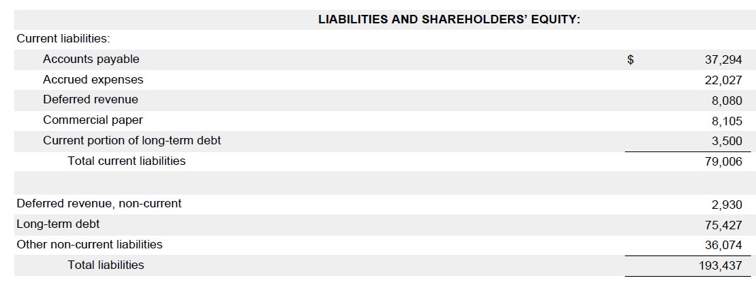
As with the non-operating assets, finance professionals usually just use the latest balance sheet values of these items as a proxy for their actual values. This is usually a safe approach when the market values are fairly close to the balance sheet values. The market value of debt doesn’t usually deviate too much from the book value unless market interest rates have changed dramatically since the issue or if the company’s credit profile has changed dramatically (i.e. a company in financial distress will have its debt trading at pennies on the dollar).

One place where the book value-as-proxy-for-market-value can be dangerous is with “non-controlling interests.” Non-controlling interests are usually understated on the balance sheet. If they are significant, it is preferable to apply an industry multiple to better reflect their true value.

The bad news is that we rarely have enough insight into the nature of the non-controlling interests’ operations to figure out the right multiple to use. The good news is that non-controlling interests are rarely large enough to make a significant difference in valuation (most companies don’t have any).

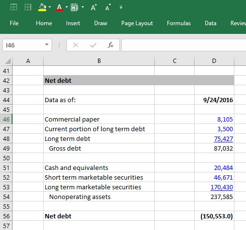
Net debt formula

When building a DCF model, finance professionals often net non-operating assets against non-equity claims and call it net debt, which is subtracted from enterprise value to arrive at equity value:

Enterprise value – net debt = Equity value

The formula for net debt is simply the value of all nonequity claims less the value of all non-operating assets:

Gross Debt (short term, long term, bonds, loans, etc..)
+ Capital Leases
+ Preferred stock
+ Non-controlling (minority) interests
– Cash
– Marketable securities
– Equity investments
Net debt

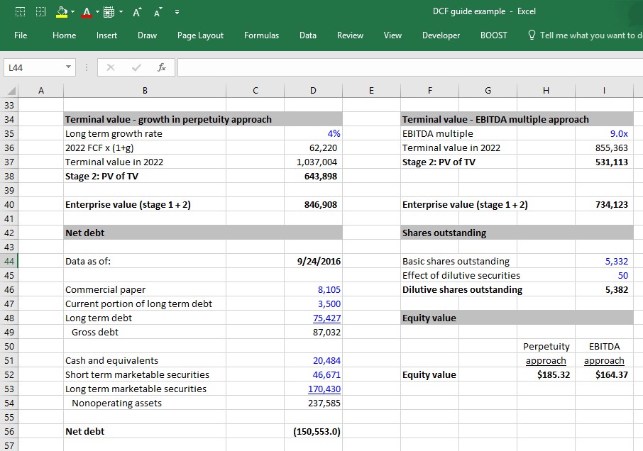
Using Apple’s 2016 10K, we can see that it has a substantial negative net debt balance. For companies that carry significant debt, a positive net debt balance is more common, while a negative net debt balance is common for companies that keep a lot of cash.

From equity value to equity value per share

Once a company’s equity value has been calculated, the next step is to determine the value of each individual share. In order to figure this out, we have to determine the number of shares that are currently outstanding. We have written a thorough guide to calculating a company’s current shares but will summarize the key steps here:

1. Take the current actual share count from the front cover of the company’s latest annual (10K) or interim (10Q) filing. For Apple, it is:

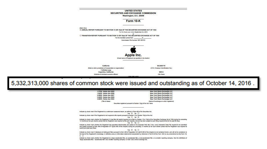
2. Next, add the effect of dilutive shares. These are shares that aren’t quite common stock yet, but that can become common stock and thus be potentially dilutive to the common shareholders (i.e. stock options, warrants, restricted stock and convertible debt and convertible preferred stock).

Assuming that we calculated 50 million dilutive securities for Apple, we can now put all the pieces together and complete the analysis:

Key DCF Assumptions

We have now completed the 6 steps to building a DCF model and have calculated the equity value of Apple.

What were the key assumptions that led us to the value we arrived at?

The three key assumptions in a DCF model are:

The operating assumptions (revenue growth and operating margins)
The WACC
Terminal value assumptions: Long-term growth rate and the exit multiple

Each of these assumptions is critical to getting an accurate model. In fact, the DCF model’s sensitivity to these assumptions, and the lack of confidence finance professionals have in these assumptions, (especially the WACC and terminal value) are frequently cited as the main weaknesses of the DCF model.

Nonetheless, the DCF model is one of the most common models used by investment bankers and other finance professionals, and the DCF output is almost always presented using a range of terminal value and WACC assumptions, as well as in context to other valuation methodologies. A common way this is presented is using a football field valuation matrix.

We wrote this guide for those thinking about a career in finance and those in the early stages of preparing for job interviews. This guide is quite detailed, but it stops short of all corner cases and nuances of a fully-fledged DCF model.

Step-by-Step Online Course

Everything You Need To Master Financial Modeling

Enroll in The Premium Package: Learn Financial Statement Modeling, DCF, M&A, LBO and Comps. The same training program used at top investment banks.

Enroll Today

Источник

Как подсчитать справедливую стоимость компании по модели DCF

Справедливой называют обоснованную цену сделки купли-продажи, устраивающую и покупателя, и продавца. О том, как выполнить расчет справедливой цены компании по модели дисконтированных денежных потоков (DCF), — в статье.

Денежный поток (cash flow) — это сумма денег, которой располагает компания после вычета всех расходов. Очевидно, что покупатель не захочет продать компанию ниже, чем текущая стоимость генерируемых ею будущих денежных потоков, а покупатель — заплатить больше этой величины. Таким образом, мы можем получить справедливую оценку стоимости бизнеса.

Как устроена модель DCF
Формула DCF
Расчет денежных потоков
Расчет ставки дисконтирования
Терминальная стоимость
Ограничения модели DCF
Пример расчета
Кратко

Как устроена модель DCF

Методика дисконтированных денежных потоков (discounted cash flow, DCF) основана на суммировании всех денежных потоков, которые компания может генерировать в будущем. Денежные потоки дисконтируются к настоящему моменту времени, поскольку стоимость денег сегодня выше, чем стоимость денег в будущем.

Модель DCF может использоваться в двух основных направлениях:

при оценке бизнеса для продажи, инвестиционных целей, при кредитовании;
при расчете справедливой стоимости акций при фундаментальном анализе.

Полученная оценка стоимости компании доходным методом не зависит от сиюминутных, конъюнктурных факторов, поскольку она основана на объективных показателях деятельности.

Метод DCF заслужил хорошую репутацию при оценке крупных, финансово устойчивых компаний, но при этом его не применяют при оценке стартапов и быстро растущих технологических компаний, которые еще не приносят прибыль.

Также этот метод стараются не использовать при оценке финансовых учреждений и управляющих компаний в сфере недвижимости.

Формула DCF

Формула расчета приведенной стоимости по модели DCF выглядит следующим образом:

где PV — это суммарная величина дисконтированных денежных потоков, генерируемых компанией за все время ее деятельности;

CFi — годовые денежные потоки в ближайшие пять лет;

r — ставка дисконтирования;

FV — суммарная величина денежных потоков за пределами прогнозного периода в настоящее время, т. н. терминальная стоимость.

Обычно в модели DCF прогнозный срок составляет пять лет, хотя в период нестабильности экономики российские эксперты закладывали в оценку компаний трехлетний прогнозный период.

Таким образом, расчет справедливой стоимости компании по методу дисконтированных денежных потоков включает следующие действия:

Анализ денежных потоков в предыдущие годы для обоснования прогнозных величин;
Прогнозирование денежных потоков на пятилетний период с учетом анализа рыночной конъюнктуры, корпоративных планов, макроэкономической ситуации и рисков;
Расчет ставки дисконтирования;
Расчет приведенной стоимости каждого расчетного годового денежного потока;
Определение темпа роста бизнеса и ставки дисконтирования в постпрогнозный период для расчета терминальной стоимости;
Суммирование дисконтированной стоимости компании в прогнозный и постпрогнозный периоды.

Спрогнозировать будущие обороты и величину ставки дисконтирования можно лишь приблизительно: качество выполненных оценок будет зависеть от квалификации экспертов и располагаемой ими информации. Поскольку объем информации о рынке и компании может существенно меняться со временем, оценка методом DCF обладает ограниченным сроком годности. Специалисты советуют обновлять оценки стоимости компании на ежегодной основе.

Расчет денежных потоков

Свободный денежный поток фирмы (FCF) определяется как разность всех поступлений и всех издержек, налогов и чистых инвестиций. При расчете неважно, приобретены ли активы на деньги акционеров или на заемные средства. Чистые инвестиции, в свою очередь, рассчитываются как суммарные капиталовложения минус амортизация и плюс увеличение оборотного капитала.

СF = EBIT* (1 – T) + D&A – CapEx – CWK,

где СF — денежный поток, EBIT — прибыль до вычета процентов и налогов, Т — налоговая ставка на прибыль, D&A — амортизационные расходы, CapEx — вложения в основные средства компании, CWK — изменения в оборотном капитале компании (увеличение оборотного капитала уменьшает денежный поток, сокращение оборотного капитала увеличивает его).

Эти данные можно взять из финансовой отчетности по международным стандартам, показатель EBIT рассчитывается вычитанием амортизации из чаще указываемого бизнес-показателя EBITDA.

Для компаний, отчитывающихся по российским стандартам бухгалтерской отчетности, денежный поток можно определить на основании данных отчета о движении денежных средств. Для этого из чистого денежного потока от операционной деятельности нужно вычесть величину капитальных затрат.

Для того чтобы обосновать величину будущих денежных потоков для модели DCF, будет полезным рассчитать денежные потоки за предыдущие три года и оценить динамику их изменений.

При анализе отчетных документов нужно изучить структуру расходов, обратив особое внимание на единовременные и чрезвычайные статьи расходов, которые встречались в прошлом, но вряд ли возникнут в будущем. Для полноценного анализа будет не лишним провести сравнение структуры расходов оцениваемой компании с соответствующими показателями конкурентов.

При прогнозе показателей будущих периодов следует учесть множество факторов, включая:

рост спроса на продукты или услуги компании,
общий рост цен,
общеэкономические и отраслевые тренды,
будущие инвестиции и отдачу от них,
конкурентные преимущества компании.

Однако в простейшем расчете можно отказаться от столь громоздкого анализа, предположив стабильный рост оборотов компании на определенную величину.

Расчет ставки дисконтирования

Ставка дисконтирования — это коэффициент, отражающий ожидаемую или требуемую ставку доходности капитала. Уровень ставки должен быть выбран таким, чтобы учитывать инфляцию и все виды рисков, присущие оцениваемому бизнесу.

В качестве ставки дисконтирования можно принять средневзвешенную стоимость совокупного капитала фирмы (weighted average cost of capital, WACC). Это усредненная стоимость собственного и заемного капиталов, где в качестве весов выступают доли собственных и заемных средств в балансе компании.

Формула расчета по методу WACC выглядит следующим образом:

WACC (%)= wd*rd*(1-T) +we*re,

где wd — доля заемного капитала в общем капитале бизнеса, rd — ставка по заемному капиталу, we — доля собственного капитала, re — ставка по собственному капиталу и T — ставка налога на прибыль.

Стоимость заемного капитала — это средние ставки по кредитам компании. В том случае, если данные по взятым компанией обязательствам недоступны, берутся рыночные ставки по кредитам для юридических лиц.

Доходность собственного капитала либо устанавливается с помощью экспертных оценок, либо рассчитывается с помощью модели CAPM (Capital Asset Pricing Model) — подробнее в статье Ставка дисконтирования: суть и методы расчета.

Терминальная стоимость

Терминальная стоимость компании равна дисконтированной на сегодняшний день сумме всех денежных потоков за пределами прогнозного периода. Обычно считается, что бизнес компании будет стабильно расти постоянными темпами, а ставка дисконтирования останется неизменной.

Расчет терминальной стоимости производят по модели Гордона:

где: FV — терминальная стоимость, r — ставка дисконтирования, t — темп прироста денежного потока компании.

Процент прироста денежных потоков не должен превышать величину ставки дисконтирования, поскольку в противном случае можно получить негативную стоимость компании.

Ограничения модели DCF

В модели DCF используется большое количество экспертных оценок, касающихся как будущих денежных потоков, так и ставки дисконтирования. При этом неправильная оценка одного из факторов может привести к существенному изменению в конечной оценке бизнеса.

Также в рамках модели полагают, что весь денежный поток будет доступен для владельцев, размер дивидендных выплат не учитывается. Кроме этого, расчет по модели DCF достаточно трудоемкий и требует умения работать с бухгалтерской отчетностью.

Терминальная стоимость нередко превышает суммарную величину приведенных денежных потоков в прогнозном периоде. Однако оценить с высокой точностью то, что будет происходить за пределами прогнозного периода, практически невозможно.

Таким образом, наибольшую точность метод DCF демонстрирует при оценке стабильно растущих компаний, с долговременными рыночными перспективами, либо тех компаний, которые созданы на проектной основе, обладающих конечным сроком деятельности.

Пример расчета

Допустим, что денежный поток компании в первый прогнозный год составит 100 млн рублей, во второй — 110, в третий — 115, в четвертый — 125, в пятый — 130 и в шестой — 140 млн рублей. Оценим стоимость компании по модели DCF, если ставка дисконтирования составляет 15%, а рост в постпрогнозном периоде составит 3%.

Тогда (в млн рублей):

В нашем примере 75% общей стоимости компании приходится на терминальную стоимость в постпрогнозном периоде.

Кратко

1
Методика дисконтированных денежных потоков (discounted cash flow, DCF) основана на суммировании всех денежных потоков, которые компания может генерировать в будущем.
2
Метод DCF заслужил хорошую репутацию при оценке крупных стабильно растущих компаний, но при этом его не применяют при оценке стартапов и быстро растущих технологических компаний, которые еще не приносят прибыль.
3
Для расчета стоимости компании по модели DCF требуется спрогнозировать денежные потоки компании на прогнозный период, вычислить ставку дисконтирования и терминальную стоимость компании.
4
Терминальная стоимость компании равна дисконтированной на сегодняшний день сумме всех денежных потоков за пределами прогнозного периода. Считается, что бизнес компании будет стабильно расти постоянными темпами, а ставка дисконтирования останется неизменной.
5
Поскольку в модели DCF используется большое количество экспертных оценок, неправильная оценка одного из факторов может привести к существенному изменению в конечной оценке бизнеса.

Данный справочный и аналитический материал подготовлен компанией ООО «Ньютон Инвестиции» исключительно в информационных целях. Оценки, прогнозы в отношении финансовых инструментов, изменении их стоимости являются выражением мнения, сформированного в результате аналитических исследований сотрудников ООО «Ньютон Инвестиции», не являются и не могут толковаться в качестве гарантий или обещаний получения дохода от инвестирования в упомянутые финансовые инструменты. Не является рекламой ценных бумаг. Не является индивидуальной инвестиционной рекомендацией и предложением финансовых инструментов. Несмотря на всю тщательность подготовки информационных материалов, «Ньютон Инвестиции» не гарантирует и не несет ответственности за их точность, полноту и достоверность.

The Big Idea Behind a DCF Model

The big idea is that you can use the following formula to value any asset or company that generates cash flow (whether now or “eventually”):

The “Discount Rate” represents risk and potential returns – a higher rate means more risk, but also higher potential returns.

A company is worth more when its cash flows and/or cash flow growth rate are higher, and it’s worth less when those are lower.

The company is also worth less when it is riskier or when expectations for it are higher, i.e., when the Discount Rate is higher.

If a company’s Discount Rate and Cash Flow Growth Rate stayed the same forever, then investment analysis would be simple: just plug the numbers into this formula.

But that never happens!

Companies grow and change over time, and often they are riskier with higher growth potential in earlier years, and then they mature and become less risky later on.

Valuation is more than this simple formula because companies’ Discount Rates and Cash Flow Growth Rates change over time.

To represent that change, you divide companies’ lifecycles into two periods:

Period #1 (Explicit Forecast Period): The company’s Cash Flow, Cash Flow Growth Rate, and potentially even the Discount Rate change over 5, 10, 15, or 20+ years, but the company reaches maturity or “stabilization” by the end.
Period #2 (Terminal Period): The Discount Rate and Cash Flow Growth Rate stop changing because the company is mature. Its Cash Flow will still change, but the valuation formula above works because it requires only the first year of Cash Flow in this period.

You value the company in both these periods and then add the results to get its total value from today into “infinity” (AKA until the Present Value of its cash flows falls to near-0).

Company/Industry Research

Before you jump into Excel and start entering numbers, you should do a bit of company and industry research to establish the following:

What are the top 5-10 most important drivers for the company?
How can you project its revenue beyond a simple percentage growth rate? What about its expenses?
What do its historical trends look like, ideally going back 5-10 years?

The company’s annual report and investor presentations are the best starting points.

You could also search for industry data from companies like IDC, Gartner, and Forrester, but it’s not necessary for a quick analysis of a mature company.

And if you are dealing with a rapidly changing company or a tech startup (e.g., Uber or Snap), it’s often more useful to get KPIs and financial stats from similar companies that were once growing quickly but have since matured.

In theory, you could spend days, weeks, or months on industry and company research, but that much effort is not necessary.

We recommend reading through the annual report and investor presentation to the extent that you can come up with those 5-10 key drivers.

For Walmart, we came up with the following:

Its annual filing repeatedly cited its total square feet, so we made the total retail square feet the top-line driver and based other numbers on $ per square foot figures.

DCF Model, Step 1: Unlevered Free Cash Flow

While there are many types of “Free Cash Flow,” in a standard DCF model, you almost always use Unlevered Free Cash Flow (UFCF), also known as Free Cash Flow to Firm (FCFF), because it produces the most consistent results and does not depend on the company’s capital structure.

Unlevered Free Cash Flow should include:

Revenue
COGS and Operating Expenses
Taxes
Depreciation & Amortization and sometimes other non-cash adjustments*
The Change in Working Capital
Capital Expenditures

*Depreciation & Amortization gets a bit more complicated, especially if you’re analyzing a company that follows IFRS (see the next section).

This list means that you ignore almost everything else: Net Interest Expense, Other Income / (Expense), most non-cash adjustments, most of the Cash Flow from Investing section, and the Cash Flow from Financing section.

For Walmart, many of the items in UFCF are simple $ per square foot figures:

To calculate UFCF, start with Revenue and subtract COGS, OpEx, and Taxes (which are now different since they’re based on Operating Income).

Then, add back D&A, factor in Deferred Taxes, any other recurring operating activities, and the Change in Working Capital, and subtract CapEx:

In some cases, we recalculate items such as Deferred Taxes because we’re modifying the company’s historical Taxes to make them comparable to future Taxes.

Most of these items should be fairly low as percentages of revenue or the change in revenue.

For example, it would be highly unusual if the Change in Working Capital represented 50% of a company’s UFCF.

For most companies, Working Capital is not a major value driver because it represents simple timing differences.

We also made sure that CapEx as a percentage of revenue stays ahead of D&A as a percentage of revenue in each year because Walmart’s cash flows are growing.

Even if the growth is modest, the company will need to increase its Net PP&E over time to support that growth.

If you don’t know what some of these items mean, please see our coverage of the Change in Working Capital and Unlevered Free Cash Flow for more details.

But Wait! What About Operating Leases in DCF Models?

Accounting for operating leases has become more complicated with the introduction of IFRS 16 in 2019, which required companies to put Operating Lease Assets and Liabilities directly on their Balance Sheets (see: our full tutorial to lease accounting).

The equivalent rules under U.S. GAAP aren’t too bad because U.S. companies still record Rent as a simple operating expense on their Income Statements.

Under IFRS, however, Rent is split into an Amortization or Depreciation element and an Interest element, similar to the treatment for Finance Leases.

Over a large portfolio of leases with different start and end dates, the Lease Amortization + Lease Interest is about the same as the Rental Expense under U.S. GAAP.

The goal in a DCF is to reflect the company’s cash revenue, cash expenses, and cash taxes, so we believe the best approach is to deduct the entire Operating Lease Expense in UFCF.

For IFRS-based companies, that means you’ll have to deduct the Interest element in the EBIT and NOPAT calculations:

Also, you should not add back the Operating Lease Depreciation or Amortization because in this case, it represents part of an actual cash expense.

If you follow this treatment, the UFCF number will reflect the deduction for the full Lease Expense.

Some argue that you should add back the entire Lease Expense and count Operating Leases as an item in the Equity Value to Enterprise Value bridge.

We don’t favor that approach because UFCF does not reflect the company’s cash expenses if you do that, and it’s more difficult to compare companies that way.

DCF Model, Step 2: The Discount Rate

Once you’ve projected the company’s Unlevered Free Cash Flows, you need to discount them to their Present Value: what they’re worth today.

That value today depends on how much you could earn with your money in other, similar companies in this market, i.e., your expected, average annualized returns.

The Discount Rate expresses these expected, average annualized returns, and in an Unlevered DCF, it’s equal to WACC, or the “Weighted Average Cost of Capital.”

The name means what it sounds like: you estimate the “cost” of each form of capital the company has, weigh them by their percentages, and then add them up.

“Capital” means “a source of funds.” So, if a company borrows money in the form of Debt to fund its operations, that Debt is a form of capital.

And if it goes public in an IPO, the shares it issues, called “Equity,” are also a form of capital.

The exact formula is:

WACC = Cost of Equity * % Equity + Cost of Debt * (1 – Tax Rate) * % Debt + Cost of Preferred Stock * % Preferred Stock

The Cost of Equity represents potential returns from the company’s stock price and dividends, or how much it “costs” the company to issue shares.

For example, if the company’s dividends are 3% of its current share price, and its stock price has increased by 6-8% each year historically, its Cost of Equity might be between 9% and 11%.

The Cost of Debt represents returns on the company’s Debt, mostly from interest, but also from the market value of the Debt changing.

For example, if the company is paying a 6% interest rate on its Debt, and the market value of its Debt is close to its face value, then the Cost of Debt might be around 6%.

You also multiply that by (1 – Tax Rate) because Interest paid on Debt is tax-deductible. So, if the Tax Rate is 25%, the After-Tax Cost of Debt would be 6% * (1 – 25%) = 4.5%.

The Cost of Preferred Stock is similar because Preferred Stock works similarly to Debt, but Preferred Stock Dividends are not tax-deductible, and overall rates tend to be higher, making it more expensive.

The Discount Rate in Real Life vs. Simple Approximations

The calculations for the Cost of Debt and Preferred Stock are straightforward, but the Cost of Equity is more challenging because it’s subjective and depends on how other, similar companies have performed relative to the market.

In many DCF models, you’ll see a sheet dedicated to this calculation, where the modeler “un-levers Beta” for each peer company to estimate its risk/volatility independent of its capital structure and then re-levers it for the subject company:

The problem with this approach is that you need quick access to data for comparable companies, which may be tricky without Capital IQ, FactSet, or similar services.

Luckily, there is a “shortcut method” as well, which involves using the same formula but simplifying the last input:

Cost of Equity = Risk-Free Rate + Equity Risk Premium * Levered Beta

The Risk-Free Rate (RFR) is what you might earn on “safe” government bonds in the same currency as the company’s cash flows (so, U.S. Treasuries here).

The Equity Risk Premium (ERP) is the percentage the stock market is expected to return each year, on average, above the yield on these “safe” government bonds.

And Levered Beta tells you how volatile this stock is relative to the market as a whole, factoring in both business risk and risk from leverage (Debt).

If it’s 1.0, then the stock follows the market perfectly and goes up by 10% when the market goes up by 10%; if it’s 2.0, the stock goes up by 20% when the market goes up by 10%.

Rather than finding comparable companies and un-levering and re-levering Beta, you could just look it up for the company on Yahoo Finance:

You can then combine it with easy-to-find data on 10-year U.S. Treasury yields and the Equity Risk Premium from Damodaran’s collection (or other sources – there are plenty of estimates for the current ERP in different markets):

The Discount Rate is around 4.0% with this approach (assuming ~90% Equity and ~10% Debt for Walmart), close to the 4.37% in the full model.

Sure, you could make it more complicated, but I would argue it’s a waste of time in a case study or modeling test unless they specifically ask for it.

The important part is that the company’s Discount Rate is closer to 5% than 10% or 15%, so we can use a range of values with 5% in the middle.

Also, you can now use this Discount Rate to take the Present Value of each UFCF (PV = UFCF / ((1 + Discount Rate) ^ Year #):

DCF Model, Step 3: The Terminal Value

The Terminal Value goes back to the “big idea” behind a DCF model.

Put simply, the “Company Value” in this formula:

IS the Terminal Value – assuming that each input represents the Terminal Period in the DCF model.

To calculate it, you need to get the company’s first Cash Flow in the Terminal Period and its Cash Flow Growth Rate and Discount Rate in that Terminal Period.

In an Unlevered DCF, this formula becomes:

Terminal Value = Unlevered FCF in Year 1 of Terminal Period / (WACC – Terminal UFCF Growth Rate)

And you can estimate the UFCF in Year 1 of the Terminal Period like this:

Terminal Value = UFCF in Final Year of Explicit Forecast Period * (1 + Terminal UFCF Growth Rate) / (WACC – Terminal UFCF Growth Rate)

This “Terminal Growth Rate” should be low: below the long-term GDP growth rate, especially in developed countries.

You could also estimate the Terminal Value with an EBITDA multiple based on median multiples from the comparable companies, but we don’t recommend that as the primary method.

It’s too easy to pick multiples that imply ridiculous Terminal FCF Growth Rates, so it’s safer to start with the growth rates and then check their implied multiples.

Once you have the Terminal Value, you can discount it back to Present Value and add it to the Sum of the Present Values of the Free Cash Flows:

And then, you can back into the Implied Equity Value and Implied Share Price from there:

You can also set up sensitivity tables to assess what the company’s valuation looks like with different assumptions for the Terminal Growth Rate, Terminal Multiple, Discount Rate, and so on:

One Final Note: This Terminal FCF Growth Rate should be fairly close to the UFCF growth rate in the final year of the explicit forecast period.

You don’t want UFCF to grow at 10% or 20% and suddenly drop to 2% in the Terminal Period.

If it does, you need to re-think your assumptions or extend the analysis.

Because of this problem, we extended the explicit forecast period to 20 years in the Uber valuation.

Conclusions from This DCF Model

Overall, Walmart seems modestly undervalued because its implied share price in most of the sensitivity tables is above its current share price of ~$140.

There is one problem with this analysis, though: we’re assuming that Walmart keeps growing its retail square feet, even though that number has been declining in recent years.

Therefore, if we had more time and resources, we might create a few operating scenarios, similar to the Uber and Snap models, to assess the results in “growth” vs. “stagnant” vs. “decline” cases.

Common Criticisms of the DCF Model – and Responses

People often criticize the DCF model for the following reasons:

“But how can you possibly predict a company 5, 10, or 15 years into the future? No one can!”
“The DCF is too sensitive to small changes in assumptions, such as growth rates and margins.”
“A DCF ignores market conditions and comparable companies, so it might not give you the accurate market value.”
“The DCF is no longer applicable because stocks are valued based on memes / crypto / Reddit! No one cares about cash flow.”

My response to the first three objections is similar: it’s not about the exact numbers but ranges, scenarios, and sensitivities.

No, you don’t know whether the Year 10 growth rate will be 10% or 8% or 12%, but you should have an idea of whether it will be closer to 10% or 20%.

And if you don’t, it’s fine to build a DCF with a wide valuation range that reflects high uncertainty.

The complaint about a DCF being “too sensitive” raises other questions: for example, is the FCF growth rate in the final year of the explicit forecast period close to the Terminal FCF Growth Rate?

If not, you need to re-think your assumptions or extend the projections.

And the critique about ignoring market conditions conveniently ignores that the Discount Rate is always based on current market conditions, no matter how you calculate it.

The DCF is indeed less reflective of the current market than comparable company analysis (for example), but it still reflects some market conditions.

And finally, for the crypto/meme/Reddit objection: yes, I agree that certain stocks seem to defy all logic and cash flow-based analysis.

That said, these stocks represent a tiny fraction of all the public companies worldwide.

The media gives them excessive attention, but they ignore the hundreds of thousands (millions?) of other companies that follow some semblance of logic.

And as for crypto, I agree that you cannot use a DCF to value Bitcoin, Ethereum, or Dogecoin.

But this is nothing new: a DCF only works for assets that generate cash flow, whether now or in the future.

No one has ever suggested valuing gold or silver with a DCF, and I’m not sure how crypto is any different in this regard.

DCF Models: Further Learning

If you want to learn more about DCF models and get a step-by-step walkthrough in more detail, sign up for our free financial modeling tutorials.

These tutorials provide a 3-part series on the valuation of Michael Hill, a retailer in Australia and New Zealand, and they go into each step in more depth than we did above.

And if you want in-depth case studies backed by real-world data and research, the Financial Modeling Mastery course delves into valuation/DCF analysis in even greater detail.

A few modules are dedicated to valuation and DCF analysis, and there are examples of company valuation in other industries (steel, pharmaceuticals, building materials, solar power, online subscription services, etc.).

—

If you liked this article, you might be interested in reading Enterprise Value vs Equity Value: The Complete Guide.

Источник

Расчет Enterprise Value

Что такое финансовый долг?

Расчет стоимости капитала

Что такое неориентированный свободный денежный поток?

Почему денежный поток дисконтируется?

Как построить прогноз денежных потоков в модели DCF

1. Прогнозирование выручки

2. Прогнозирование расходов

3. Прогнозирование капитальных активов и изменений в оборотном капитале

4. Прогнозирование структуры капитала

5. Терминальная стоимость

6. Сроки денежных потоков

7. DCF Стоимость предприятия

8. DCF Стоимость акционерного капитала

Анализ чувствительности в модели DCF

Дополнительные ресурсы:

What is a DCF Model?

DCF Model Basics: Present Value Formula

DCF Model in Excel – Sample Template Download

How to Build a DCF Model: 6-Step Framework

Step 1. Forecasting unlevered free cash flows

Step 2. Calculating the terminal value

Step 3. Discounting the cash flows to the present at the weighted average cost of capital

Step 4. Add the value of non-operating assets to the present value of unlevered free cash flows

Step 5. Subtract debt and other non-equity claims

Step 6. Divide the equity value by the shares outstanding

Calculating Unlevered Free Cash Flows (FCF)

FCFs are ideally driven from a 3-statement model

The 2-stage DCF model

Calculating the terminal value

The growth in perpetuity approach

Exit EBITDA Multiple Method

Growth in perpetuity vs. exit EBITDA multiple method

Getting to enterprise value: Discounting the cash flows by the WACC

Getting to equity value: Adding the value of non-operating assets

Getting to equity value: Subtracting debt and other non-equity claims

From equity value to equity value per share

Key DCF Assumptions

Everything You Need To Master Financial Modeling

Как устроена модель DCF

Формула DCF

Расчет денежных потоков

Расчет ставки дисконтирования

Терминальная стоимость

Ограничения модели DCF

Пример расчета

Кратко

Читайте также

The Big Idea Behind a DCF Model

Company/Industry Research

DCF Model, Step 1: Unlevered Free Cash Flow

But Wait! What About Operating Leases in DCF Models?

DCF Model, Step 2: The Discount Rate

The Discount Rate in Real Life vs. Simple Approximations

DCF Model, Step 3: The Terminal Value

Conclusions from This DCF Model

Common Criticisms of the DCF Model – and Responses

DCF Models: Further Learning