Коэффициент теплопередачи как его найти - Исправление недочетов и поиск решений вместе с Examum.ru

In thermodynamics, the heat transfer coefficient or film coefficient, or film effectiveness, is the proportionality constant between the heat flux and the thermodynamic driving force for the flow of heat (i.e., the temperature difference, ΔT ). It is used in calculating the heat transfer, typically by convection or phase transition between a fluid and a solid. The heat transfer coefficient has SI units in watts per square meter per kelvin (W/m²/K).

The overall heat transfer rate for combined modes is usually expressed in terms of an overall conductance or heat transfer coefficient, U. In that case, the heat transfer rate is:

${displaystyle {dot {Q}}=hA(T_{2}-T_{1})}$

where (in SI units):

A: surface area where the heat transfer takes place (m²)
T₂: temperature of the surrounding fluid (K)
T₁: temperature of the solid surface (K)

The general definition of the heat transfer coefficient is:

$h = frac{q}{Delta T}$

where:

q: heat flux (W/m²); i.e., thermal power per unit area,
ΔT: difference in temperature between the solid surface and surrounding fluid area (K)

The heat transfer coefficient is the reciprocal of thermal insulance. This is used for building materials (R-value) and for clothing insulation.

There are numerous methods for calculating the heat transfer coefficient in different heat transfer modes, different fluids, flow regimes, and under different thermohydraulic conditions. Often it can be estimated by dividing the thermal conductivity of the convection fluid by a length scale. The heat transfer coefficient is often calculated from the Nusselt number (a dimensionless number). There are also online calculators available specifically for Heat-transfer fluid applications. Experimental assessment of the heat transfer coefficient poses some challenges especially when small fluxes are to be measured (e.g. < 0.2 W/cm²).^[1]^[2]

Composition[edit]

A simple method for determining an overall heat transfer coefficient that is useful to find the heat transfer between simple elements such as walls in buildings or across heat exchangers is shown below. Note that this method only accounts for conduction within materials, it does not take into account heat transfer through methods such as radiation. The method is as follows:

${displaystyle {frac {1}{Ucdot A}}={frac {1}{h_{1}cdot A_{1}}}+{frac {dx_{w}}{kcdot A}}+{frac {1}{h_{2}cdot A_{2}}}}$

Where:

As the areas for each surface approach being equal the equation can be written as the transfer coefficient per unit area as shown below:

${displaystyle {frac {1}{U}}={frac {1}{h_{1}}}+{frac {dx_{w}}{k}}+{frac {1}{h_{2}}}}$

${displaystyle U={frac {1}{{frac {1}{h_{1}}}+{frac {dx_{w}}{k}}+{frac {1}{h_{2}}}}}}$

Often the value for $dx_{w}$ is referred to as the difference of two radii where the inner and outer radii are used to define the thickness of a pipe carrying a fluid, however, this figure may also be considered as a wall thickness in a flat plate transfer mechanism or other common flat surfaces such as a wall in a building when the area difference between each edge of the transmission surface approaches zero.

In the walls of buildings the above formula can be used to derive the formula commonly used to calculate the heat through building components. Architects and engineers call the resulting values either the U-Value or the R-Value of a construction assembly like a wall. Each type of value (R or U) are related as the inverse of each other such that R-Value = 1/U-Value and both are more fully understood through the concept of an overall heat transfer coefficient described in lower section of this document.

Convective heat transfer correlations[edit]

Although convective heat transfer can be derived analytically through dimensional analysis, exact analysis of the boundary layer, approximate integral analysis of the boundary layer and analogies between energy and momentum transfer, these analytic approaches may not offer practical solutions to all problems when there are no mathematical models applicable. Therefore, many correlations were developed by various authors to estimate the convective heat transfer coefficient in various cases including natural convection, forced convection for internal flow and forced convection for external flow. These empirical correlations are presented for their particular geometry and flow conditions. As the fluid properties are temperature dependent, they are evaluated at the film temperature $T_{f}$ , which is the average of the surface $T_{s}$ and the surrounding bulk temperature, ${{T}_{{infty }}}$ .

${{T}_{{f}}}={frac {{{T}_{{s}}}+{{T}_{{infty }}}}{2}}$

External flow, vertical plane[edit]

Recommendations by Churchill and Chu provide the following correlation for natural convection adjacent to a vertical plane, both for laminar and turbulent flow.^[3]^[4] k is the thermal conductivity of the fluid, L is the characteristic length with respect to the direction of gravity, Ra_L is the Rayleigh number with respect to this length and Pr is the Prandtl number.
(Note: The Rayleigh number can be written as the product of the Grashof number and the Prandtl number)

${displaystyle h ={frac {k}{L}}left({0.825+{frac {0.387mathrm {Ra} _{L}^{1/6}}{left(1+(0.492/mathrm {Pr} )^{9/16}right)^{8/27}}}}right)^{2},quad mathrm {Ra} _{L}<10^{12}}$

For laminar flows, the following correlation is slightly more accurate. It is observed that a transition from a laminar to a turbulent boundary occurs when Ra_L exceeds around 10⁹.

${displaystyle h ={frac {k}{L}}left(0.68+{frac {0.67mathrm {Ra} _{L}^{1/4}}{left(1+(0.492/mathrm {Pr} )^{9/16}right)^{4/9}}}right),quad mathrm {1} 0^{-1}<mathrm {Ra} _{L}<10^{9}}$

External flow, vertical cylinders[edit]

For cylinders with their axes vertical, the expressions for plane surfaces can be used provided the curvature effect is not too significant. This represents the limit where boundary layer thickness is small relative to cylinder diameter . The correlations for vertical plane walls can be used when

${displaystyle {frac {D}{L}}geq {frac {35}{mathrm {Gr} _{L}^{frac {1}{4}}}}}$

where ${displaystyle mathrm {Gr} _{L}}$ is the Grashof number.

External flow, horizontal plates[edit]

W. H. McAdams suggested the following correlations for horizontal plates.^[5] The induced buoyancy will be different depending upon whether the hot surface is facing up or down.

For a hot surface facing up, or a cold surface facing down, for laminar flow:

${displaystyle h ={frac {k0.54mathrm {Ra} _{L}^{1/4}}{L}},quad 10^{5}<mathrm {Ra} _{L}<2times 10^{7}}$

and for turbulent flow:

${displaystyle h ={frac {k0.14mathrm {Ra} _{L}^{1/3}}{L}},quad 2times 10^{7}<mathrm {Ra} _{L}<3times 10^{10}.}$

For a hot surface facing down, or a cold surface facing up, for laminar flow:

${displaystyle h ={frac {k0.27mathrm {Ra} _{L}^{1/4}}{L}},quad 3times 10^{5}<mathrm {Ra} _{L}<3times 10^{10}.}$

The characteristic length is the ratio of the plate surface area to perimeter. If the surface is inclined at an angle θ with the vertical then the equations for a vertical plate by Churchill and Chu may be used for θ up to 60°; if the boundary layer flow is laminar, the gravitational constant g is replaced with g cos θ when calculating the Ra term.

External flow, horizontal cylinder[edit]

For cylinders of sufficient length and negligible end effects, Churchill and Chu has the following correlation for $10^{{-5}}<{mathrm {Ra}}_{D}<10^{{12}}$ .

${displaystyle h ={frac {k}{D}}left({0.6+{frac {0.387mathrm {Ra} _{D}^{1/6}}{left(1+(0.559/mathrm {Pr} )^{9/16},right)^{8/27},}}}right)^{2}}$

External flow, spheres[edit]

For spheres, T. Yuge has the following correlation for Pr≃1 and $1leq {mathrm {Ra}}_{D}leq 10^{5}$ .^[6]

${displaystyle {mathrm {Nu} }_{D} =2+0.43mathrm {Ra} _{D}^{1/4}}$

Vertical rectangular enclosure[edit]

For heat flow between two opposing vertical plates of rectangular enclosures, Catton recommends the following two correlations for smaller aspect ratios.^[7] The correlations are valid for any value of Prandtl number.

For ${displaystyle 1<{frac {H}{L}}<2}$ :

${displaystyle h ={frac {k}{L}}0.18left({frac {mathrm {Pr} }{0.2+mathrm {Pr} }}mathrm {Ra} _{L}right)^{0.29},quad mathrm {Ra} _{L}mathrm {Pr} /(0.2+mathrm {Pr} )>10^{3}}$

where H is the internal height of the enclosure and L is the horizontal distance between the two sides of different temperatures.

For ${displaystyle 2<{frac {H}{L}}<10}$ :

${displaystyle h ={frac {k}{L}}0.22left({frac {mathrm {Pr} }{0.2+mathrm {Pr} }}mathrm {Ra} _{L}right)^{0.28}left({frac {H}{L}}right)^{-1/4},quad mathrm {Ra} _{L}<10^{10}.}$

For vertical enclosures with larger aspect ratios, the following two correlations can be used.^[7] For 10 < H/L < 40:

${displaystyle h ={frac {k}{L}}0.42mathrm {Ra} _{L}^{1/4}mathrm {Pr} ^{0.012}left({frac {H}{L}}right)^{-0.3},quad 1<mathrm {Pr} <2times 10^{4},,quad 10^{4}<mathrm {Ra} _{L}<10^{7}.}$

For ${displaystyle 1<{frac {H}{L}}<40}$ :

${displaystyle h ={frac {k}{L}}0.46mathrm {Ra} _{L}^{1/3},quad 1<mathrm {Pr} <20,,quad 10^{6}<mathrm {Ra} _{L}<10^{9}.}$

For all four correlations, fluid properties are evaluated at the average temperature—as opposed to film temperature— ${displaystyle (T_{1}+T_{2})/2}$ , where $T_{1}$ and $T_{2}$ are the temperatures of the vertical surfaces and .

Forced convection[edit]

Internal flow, laminar flow[edit]

Sieder and Tate give the following correlation to account for entrance effects in laminar flow in tubes where is the internal diameter, ${mu }_{{b}}$ is the fluid viscosity at the bulk mean temperature, ${mu }_{{w}}$ is the viscosity at the tube wall surface temperature.^[6]

${displaystyle mathrm {Nu} _{D}={1.86}cdot {{left(mathrm {Re} cdot mathrm {Pr} right)}^{{}^{1}!!diagup !!{}_{3};}}{{left({frac {D}{L}}right)}^{{}^{1}!!diagup !!{}_{3};}}{{left({frac {{mu }_{b}}{{mu }_{w}}}right)}^{0.14}}}$

For fully developed laminar flow, the Nusselt number is constant and equal to 3.66. Mills combines the entrance effects and fully developed flow into one equation

${displaystyle mathrm {Nu} _{D}=3.66+{frac {0.065cdot mathrm {Re} cdot mathrm {Pr} cdot {frac {D}{L}}}{1+0.04cdot left(mathrm {Re} cdot mathrm {Pr} cdot {frac {D}{L}}right)^{2/3}}}}$

^[8]

Internal flow, turbulent flow[edit]

The Dittus-Bölter correlation (1930) is a common and particularly simple correlation useful for many applications. This correlation is applicable when forced convection is the only mode of heat transfer; i.e., there is no boiling, condensation, significant radiation, etc. The accuracy of this correlation is anticipated to be ±15%.

For a fluid flowing in a straight circular pipe with a Reynolds number between 10,000 and 120,000 (in the turbulent pipe flow range), when the fluid’s Prandtl number is between 0.7 and 120, for a location far from the pipe entrance (more than 10 pipe diameters; more than 50 diameters according to many authors^[9]) or other flow disturbances, and when the pipe surface is hydraulically smooth, the heat transfer coefficient between the bulk of the fluid and the pipe surface can be expressed explicitly as:

${hd over k}={0.023},left({jd over mu }right)^{{0.8}},left({mu c_{p} over k}right)^{n}$

where:

is the hydraulic diameter

is the thermal conductivity of the bulk fluid

is the fluid viscosity

mass flux

$c_{p}$

isobaric heat capacity of the fluid

is 0.4 for heating (wall hotter than the bulk fluid) and 0.33 for cooling (wall cooler than the bulk fluid).^[10]

The fluid properties necessary for the application of this equation are evaluated at the bulk temperature thus avoiding iteration.

Forced convection, external flow[edit]

In analyzing the heat transfer associated with the flow past the exterior surface of a solid, the situation is complicated by phenomena such as boundary layer separation. Various authors have correlated charts and graphs for different geometries and flow conditions.
For flow parallel to a plane surface, where is the distance from the edge and is the height of the boundary layer, a mean Nusselt number can be calculated using the Colburn analogy.^[6]

Thom correlation[edit]

There exist simple fluid-specific correlations for heat transfer coefficient in boiling. The Thom correlation is for the flow of boiling water (subcooled or saturated at pressures up to about 20 MPa) under conditions where the nucleate boiling contribution predominates over forced convection. This correlation is useful for rough estimation of expected temperature difference given the heat flux:^[11]

${displaystyle Delta T_{rm {sat}}=22.5cdot {q}^{0.5}exp(-P/8.7)}$

where:

${displaystyle Delta T_{rm {sat}}}$

is the wall temperature elevation above the saturation temperature, K

q is the heat flux, MW/m²

P is the pressure of water, MPa

Note that this empirical correlation is specific to the units given.

Heat transfer coefficient of pipe wall[edit]

The resistance to the flow of heat by the material of pipe wall can be expressed as a «heat transfer coefficient of the pipe wall». However, one needs to select if the heat flux is based on the pipe inner or the outer diameter.
Selecting to base the heat flux on the pipe inner diameter, and assuming that the pipe wall thickness is small in comparison with the pipe inner diameter, then the heat transfer coefficient for the pipe wall can be calculated as if the wall were not curved^{[citation needed]}:

${displaystyle h_{rm {wall}}={2k over x}}$

where k is the effective thermal conductivity of the wall material and x is the wall thickness.

If the above assumption does not hold, then the wall heat transfer coefficient can be calculated using the following expression:

${displaystyle h_{rm {wall}}={2k over {d_{rm {i}}ln(d_{rm {o}}/d_{rm {i}})}}}$

where d_i and d_o are the inner and outer diameters of the pipe, respectively.

The thermal conductivity of the tube material usually depends on temperature; the mean thermal conductivity is often used.

Combining convective heat transfer coefficients[edit]

For two or more heat transfer processes acting in parallel, convective heat transfer coefficients simply add:

$h=h_{1}+h_{2}+cdots$

For two or more heat transfer processes connected in series, convective heat transfer coefficients add inversely:^[12]

${1 over h}={1 over h_{1}}+{1 over h_{2}}+dots$

For example, consider a pipe with a fluid flowing inside. The approximate rate of heat transfer between the bulk of the fluid inside the pipe and the pipe external surface is:^[13]

q=left({1 over {{1 over h}+{t over k}}}right)cdot Acdot Delta T

where

q = heat transfer rate (W)

h = convective heat transfer coefficient (W/(m²·K))

t = wall thickness (m)

k = wall thermal conductivity (W/m·K)

A = area (m²)

= difference in temperature.

Overall heat transfer coefficient[edit]

The overall heat transfer coefficient is a measure of the overall ability of a series of conductive and convective barriers to transfer heat. It is commonly applied to the calculation of heat transfer in heat exchangers, but can be applied equally well to other problems.

For the case of a heat exchanger, can be used to determine the total heat transfer between the two streams in the heat exchanger by the following relationship:

$q=UADelta T_{{LM}}$

where:

= heat transfer rate (W)

= overall heat transfer coefficient (W/(m²·K))

= heat transfer surface area (m²)

$Delta T_{{LM}}$

= logarithmic mean temperature difference (K).

The overall heat transfer coefficient takes into account the individual heat transfer coefficients of each stream and the resistance of the pipe material. It can be calculated as the reciprocal of the sum of a series of thermal resistances (but more complex relationships exist, for example when heat transfer takes place by different routes in parallel):

${frac {1}{UA}}=sum {frac {1}{hA}}+sum R$

where:

R = Resistance(s) to heat flow in pipe wall (K/W)

Other parameters are as above.^[14]

The heat transfer coefficient is the heat transferred per unit area per kelvin. Thus area is included in the equation as it represents the area over which the transfer of heat takes place. The areas for each flow will be different as they represent the contact area for each fluid side.

The thermal resistance due to the pipe wall (for thin walls) is calculated by the following relationship:

${displaystyle R={frac {x}{k}}}$

where

x = the wall thickness (m)

k = the thermal conductivity of the material (W/(m·K))

This represents the heat transfer by conduction in the pipe.

The thermal conductivity is a characteristic of the particular material. Values of thermal conductivities for various materials are listed in the list of thermal conductivities.

As mentioned earlier in the article the convection heat transfer coefficient for each stream depends on the type of fluid, flow properties and temperature properties.

Some typical heat transfer coefficients include:

Air — h = 10 to 100 W/(m²K)
Water — h = 500 to 10,000 W/(m²K).

Thermal resistance due to fouling deposits[edit]

Often during their use, heat exchangers collect a layer of fouling on the surface which, in addition to potentially contaminating a stream, reduces the effectiveness of heat exchangers. In a fouled heat exchanger the buildup on the walls creates an additional layer of materials that heat must flow through. Due to this new layer, there is additional resistance within the heat exchanger and thus the overall heat transfer coefficient of the exchanger is reduced. The following relationship is used to solve for the heat transfer resistance with the additional fouling resistance:^[15]

${frac {1}{U_{{f}}P}}$

= ${frac {1}{UP}}+{frac {R_{{fH}}}{P_{{H}}}}+{frac {R_{{fC}}}{P_{{C}}}}$

where

$U_{{f}}$

= overall heat transfer coefficient for a fouled heat exchanger, ${displaystyle textstyle {rm {frac {W}{m^{2}K}}}}$

= perimeter of the heat exchanger, may be either the hot or cold side perimeter however, it must be the same perimeter on both sides of the equation,

= overall heat transfer coefficient for an unfouled heat exchanger, ${displaystyle textstyle {rm {frac {W}{m^{2}K}}}}$

$R_{{fC}}$

= fouling resistance on the cold side of the heat exchanger, ${displaystyle textstyle {rm {frac {m^{2}K}{W}}}}$

$R_{{fH}}$

= fouling resistance on the hot side of the heat exchanger, ${displaystyle textstyle {rm {frac {m^{2}K}{W}}}}$

$P_{C}$

= perimeter of the cold side of the heat exchanger,

$P_{H}$

= perimeter of the hot side of the heat exchanger,

This equation uses the overall heat transfer coefficient of an unfouled heat exchanger and the fouling resistance to calculate the overall heat transfer coefficient of a fouled heat exchanger. The equation takes into account that the perimeter of the heat exchanger is different on the hot and cold sides. The perimeter used for the does not matter as long as it is the same. The overall heat transfer coefficients will adjust to take into account that a different perimeter was used as the product will remain the same.

The fouling resistances can be calculated for a specific heat exchanger if the average thickness and thermal conductivity of the fouling are known. The product of the average thickness and thermal conductivity will result in the fouling resistance on a specific side of the heat exchanger.^[15]

$R_{f}$

= ${frac {d_{f}}{k_{f}}}$

where:

$d_{f}$

= average thickness of the fouling in a heat exchanger,

= thermal conductivity of the fouling, ${displaystyle textstyle {rm {frac {W}{mK}}}}$

References[edit]

^ Chiavazzo, Eliodoro; Ventola, Luigi; Calignano, Flaviana; Manfredi, Diego; Asinari, Pietro (2014). «A sensor for direct measurement of small convective heat fluxes: Validation and application to micro-structured surfaces» (PDF). Experimental Thermal and Fluid Science. 55: 42–53. doi:10.1016/j.expthermflusci.2014.02.010.
^ Maddox, D.E.; Mudawar, I. (1989). «Single- and Two-Phase Convective Heat Transfer From Smooth and Enhanced Microelectronic Heat Sources in a Rectangular Channel». Journal of Heat Transfer. 111 (4): 1045–1052. doi:10.1115/1.3250766.
^ Churchill, Stuart W.; Chu, Humbert H.S. (November 1975). «Correlating equations for laminar and turbulent free convection from a vertical plate». International Journal of Heat and Mass Transfer. 18 (11): 1323–1329. doi:10.1016/0017-9310(75)90243-4.
^ Sukhatme, S. P. (2005). A Textbook on Heat Transfer (Fourth ed.). Universities Press. pp. 257–258. ISBN 978-8173715440.
^ McAdams, William H. (1954). Heat Transmission (Third ed.). New York: McGraw-Hill. p. 180.
^ ^a ^b ^c James R. Welty; Charles E. Wicks; Robert E. Wilson; Gregory L. Rorrer (2007). Fundamentals of Momentum, Heat and Mass transfer (5th ed.). John Wiley and Sons. ISBN 978-0470128688.
^ ^a ^b Çengel, Yunus. Heat and Mass Transfer (Second ed.). McGraw-Hill. p. 480.
^ Subramanian, R. Shankar. «Heat Transfer in Flow Through Conduits» (PDF). clarkson.edu.
^ S. S. Kutateladze; V. M. Borishanskii (1966). A Concise Encyclopedia of Heat Transfer. Pergamon Press.
^ F. Kreith, ed. (2000). The CRC Handbook of Thermal Engineering. CRC Press.
^ W. Rohsenow; J. Hartnet; Y. Cho (1998). Handbook of Heat Transfer (3rd ed.). McGraw-Hill.
^ This relationship is similar to the harmonic mean; however, note that it is not multiplied with the number n of terms.
^ «Heat transfer between the bulk of the fluid inside the pipe and the pipe external surface». physics.stackexchange.com. Retrieved 15 December 2014.
^ Coulson and Richardson, «Chemical Engineering», Volume 1, Elsevier, 2000
^ ^a ^b A.F. Mills (1999). Heat Transfer (second ed.). Prentice Hall, Inc.

External links[edit]

Overall Heat Transfer Coefficients
Overall Heat Transfer Coefficients Table and Equation
Correlations for Convective Heat Transfer

Источник

Коэффициент
теплопередачи k
(Вт/м²К) от
горячей среды к холодной зависит от
коэффициентов α₁
и α₂
(Вт/м²К)
и термического сопротивления R
(м К/Вт)
стенки соответствующего аппарата
(трубы, пластины).

Средний
для аппарата коэффициент теплопередачи
находят из уравнения [9]

,
(3.21)

где
F_n
– площади
участков (м²)
с постоянными коэффициентами теплопередачи
k
(Вт/м²°К).

В
пластинчатых аппаратах коэффициент
теплопередачи находят по формулам для
плоской стенки

,
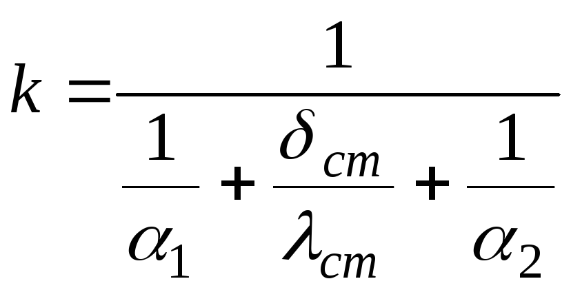(3.22)

где
a₁
и a₂
– средние значения коэффициентов
теплоотдачи от горячего теплоносителя
к стенке и от стенки к холодному
теплоносителю, Вт/м²
К;

d_с_т
– толщина поверхности стенки, м;

l_с_т
– коэффициент теплопроводности
материала, из которого изготовлена
стенка, Вт/м К.

При
проведении тепловых расчетов трубчатых
теплообменников возможно использование
формулы для плоской стенки, за исключением
труб с ребристыми поверхностями и
толстостенных гладких труб, для которых
отношение d_нр/d_вн
> 1,5.

В
практике расчетов применительно к
трубчатым теплообменникам коэффициент
теплопередачи k
относят к
наружной или внутренней поверхностям
трубы. В этом случае уравнение приобретает
вид

	(3.23)
или

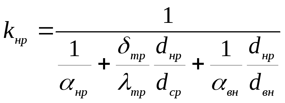
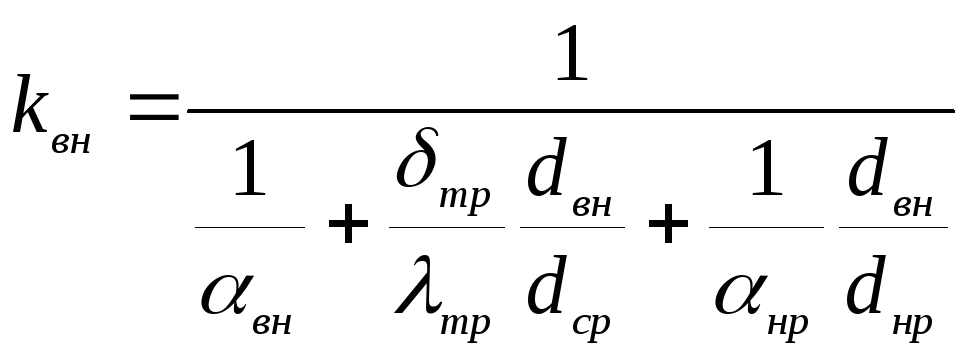
где
индексы вн,
ср,
нр
обозначают внутреннюю, среднюю и наружную
поверхности.

При
проектировании вновь создаваемого
аппарата нужно предусмотреть возможность
загрязнения с
учетом так
называемого коэффициента загрязнения
η_загр.
Расчетное значение коэффициента
теплопередачи k
определяется

k_расч
= η_загр·
k
, Вт/м²К
, (3.24)

применительно
к вязким жидкостям η_загр·=
0,65–0,85,

Расчет
ребристых поверхностей производится
по формулам теплопередачи, в которых
используются численные значения
коэффициентов теплоотдачи, справедливые,
как правило, для определенного диапазона
условий (чаще всего чисел Re)
и определяемые из опытов для конкретных
условий работы ребристых теплообменных
аппаратов [8].

Коэффициент
теплопередачи через ребристую стенку
зависит от площадей теплоотдающих
поверхностей и коэффициентов теплоотдачи
с обеих сторон стенки, толщины последней,
теплопроводности материала стенки и
загрязнений, возможных с обеих ее сторон.

Количество теплоты,
Вт, передаваемое через ребристую
поверхность, можно представить в виде

, (3.25)

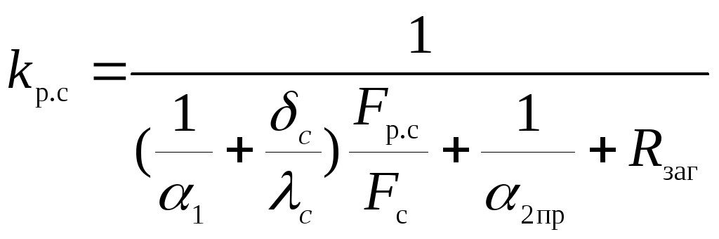
где
k_р.с
– коэффициент теплопередачи через
ребристую стенку,
Вт/м²К;

t_cp₁
и t_ср2
– средние температуры теплоносителей,
°С;

F_р.с= F_р
+ F_п
– площадь ребристой поверхности стенки,
м²,
равная сумме площади ребер F_р
и площади стенки в промежутках между
ребрами F_п.

коэффициент
теплопередачи через ребристую стенку
находим как,

, (3.26)

где
α₁
– коэффициент теплоотдачи с гладкой
стороны, Вт/(м²·К)

δ_с
– толщина материала стенки, м;

λ_с
– коэффициент теплопроводности материала
стенки, Вт/(м·К);

F_c
– площадь гладкой поверхности стенки,
м²;

α_2пр
– приведенный коэффициент теплоотдачи
со стороны ребристой поверхности,
Вт/(м²·К);

R_заг–
термическое сопротивление загрязнений
ребристой поверхности, м²
К/Вт;

Термические
сопротивления слоев загрязнений
учитываются в зависимости от того, с
какой стороны они находятся, величиной
δ’/λ’·F₁
или δ»/λ»·F₂
или их суммой, если загрязнение имеется
с обеих сторон.

Расчетный,
или приведенный, коэффициент теплоотдачи
ребристой поверхности α_2пр,
отнесенный к внешней (ребристой)
поверхности нагрева и учитывающий
неравномерность теплообмена по
поверхности ребра, определяется из
уравнения

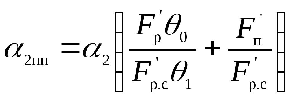, (3.27)

где
α₂
– коэффициент теплоотдачи к воздуху
от поверхности, свободной от ребер,
определяемый по критериальному уравнению,
соответствующему условиям теплообмена
стенки со средой;

F‘_p
– поверхность ребер на 1 м длины, м²/м;

F‘_п
– внешняя поверхность, не занятая
ребрами, на 1 м длины, м²/м;

F‘_p_.с
– полная внешняя поверхность 1 м длины
теплообменного аппарата, м;

θ₁–
разность между температурами основной
поверхности теплообменного аппарата
и воздуха;

θ₀
– разность между температурами
поверхности ребер и воздуха, меньшая,
чем θ₁,
вследствие изменения температуры на
поверхности ребер.

Отношение
θ₀/θ₁
находится как функция конкретных условий
обтекания ребристой поверхности α₂,
материала ребер λ_p
и их геометрии (толщины, высоты и
расположения на оребренной поверхности).

Расчет
оребренной поверхности сложен, поскольку
для его проведения необходим обширный
справочный материал, включающий в себя
вспомогательные формулы и константы
для всевозможных условий обтекания.
При оребрении стремятся к выполнению
условия α₁
F‘_с≈α₂
F‘_p_.с.

Отношение
величин оребренной поверхности F_p_._c
и гладкой F_c
называют коэффициентом оребрения и
выбирают обычно в пределах конструктивных
возможностей от 4 до 10.

Коэффициенты
теплоотдачи и их определение. При
расчетах коэффициентов теплоотдачи
необходимо знать условия движения
теплоносителей, род теплоносителей, их
физические свойства и параметры
обменивающихся теплом сред.

Соответственно
характеру и особенностям движения
теплоносителей и определяются коэффициенты
теплоотдачи сред, характеризующих
интенсивность теплообмена на границе
горячий теплоноситель-стенка и
стенка-холодный теплоноситель.

Применительно
к основным случаям теплообмена используют
критериальные уравнения, которые
получены в результате обобщения
результатов опытных исследований и
использования теории подобия [5].

Соседние файлы в предмете [НЕСОРТИРОВАННОЕ]

Источник

Вопрос от читателя нашего портала: Что такое коэффициент теплопередачи и как его рассчитать?

Ответ: Если вы планируете проживать в вашем доме зимой, важно помнить о таком важном параметре, как коэффициент теплопередачи. Для чего он нужен? Чем ниже его значение, тем меньше тепловые потери у вашего дома и, как следствие, меньше счета за его отопление.

Важно понимать, что зимой в большинстве российских коттеджей не все тепло остается внутри дома, приличная его часть уходит наружу — на улицу. Тепло из дома уходит через стены, окна и даже крышу. И размеры теплопотерь могут быть очень существенными (вплоть до 70-80%). То есть работа вашего котла и батарей в этом случае эффективна лишь на 20-30%. И именно настолько вы переплачиваете за отопление вашего дома.

Как же снизить эти теплопотери? Только качественной теплоизоляцией стен, фундамента, крыши. Так, к примеру, укладка минеральной ваты на крышу и перекрытия на чердаке снижает теплопотери домов до 40% (!), а эффективная изоляция стен, окон и потолка сводит их к минимуму.

Как же все это инженеры посчитали? Очень просто — рассчитывая коэффициент теплопередачи материалов.

Что такое коэффициент теплопередачи?

Данный коэффициент определяет количество теплового потока, проходящего через единицу площади стены или перегородки (или иной конструкции) здания, если с обеих сторон от нее имеется разница температур в 1 К (Кельвин).

Проще говоря, коэффициент теплопередачи показывает, сколько тепловой энергии проходит через ограждающую конструкцию здания. Чем ниже значение этого коэффициента, тем меньше тепловые потери. Чем выше — тем больше. В домах с высоким коэффициентом теплопередачи обычно холоднее зимой, а отопить их гораздо дороже и сложнее.

Коэффициент теплопередачи — это, пожалуй, наиболее важный параметр, используемый для определения качества теплоизоляции здания. Он обозначается символом U. Для расчета коэффициента теплопередачи следует учитывать такие факторы, как толщина стен и перегородок, их слоев и теплопроводность используемого материала.

Какое значение теплопроводности стен можно считать нормой?

В России строгих стандартов (пока что) на этот счет нет. Поэтому давайте возьмем в качестве образца нормы теплопроводности для наружных стен, используемых в странах Европы. Они следующие:

при температуре выше 16 ℃ — 0,23 Вт / (м2 · К);
при температуре от 8 до 16 ℃ — 0,45 Вт / (м2 · К);
при температуре ниже 8 ℃ — 0,90 Вт / (м2 · К).

Нормы касательно теплопроводности внутренних стен:

при температуре выше 8 ℃ и в случае стен, отделяющих отапливаемые помещения от лестничных клеток и коридоров — 1,00 Вт / (м2 · К);
при температуре ниже 8 ℃ — требований нет;
если речь идет о стенах, разделяющих нагретую и неотапливаемую части дома — 0,30 Вт / (м2 · К).

Расчет коэффициента теплопередачи

Для расчета значения коэффициента теплоотдачи дома можно воспользоваться упрощенной формулой. Она не требует особых математических знаний и такой расчет легко сделать самостоятельно.

Первым шагом является определение термического сопротивления, которое выражается символом R. Для его расчета используется формула:

R = d / λ,

где d — толщина слоя материала, выраженная в метрах;
а λ (лямбда) — это коэффициент теплопроводности материала.

Это стандартная формула, которая вошла в обиход застройщиков. Сегодня многие производители утеплителей стараются указывать эти параметры на упаковке своего товара.

Следующим шагом является вычисление общего коэффициента теплопередачи. Общая формула такая:

R + Rsi + Rse

где Rsi — коэффициент теплопередачи снаружи;
а Rse — коэффициент теплопередачи изнутри.

Для чего нужна эта формула? Она определяет окончательное значение термического сопротивления (R1).

Коэффициент теплопередачи тесно связан с проводимостью материала, поэтому он зависит от используемого материала. Информацию об этом можно найти на этикетках продукта и в технической спецификации.

Последним шагом для расчета коэффициента теплопередачи является использование формулы:

U = d / R1

где d — толщина стены или перегородки, выраженная в метрах;
а R1 — полное тепловое сопротивление.

Полученный результат следует сравнить с допустимым пределом фактора. Если стена в вашем доме состоит из нескольких слоев, отличающихся друг от друга, коэффициент следует рассчитывать отдельно для каждого из них.

Непросто и сложно? Возможно. Однако экономия в десятки тысяч рублей в год на отоплении дома в год того стоит. К тому же, вам вовсе необязательно считать все эти данные в уме или на обычном калькуляторе — сегодня в Интернете есть множество онлайн-калькуляторов, которые сделают эти расчеты за вас.

Какие материалы уменьшают теплопотери?

Чтобы снизить размер теплопотерь дома, нужно в первую очередь обратить внимание на строительные материалы, из которых строится ваш дом. Так, к примеру пеноблоки лучше сохраняют тепло, чем керамзитобетон, а пеноплостирол считается более эффективным теплоизолятором, чем минеральная вата. Узнать больше о теплопроводности материалов вы сможете на страницах нашего сайта.

Кроме того, многие производители стройматериалов указывают информацию о коэффициенте теплопередачи на упаковке. Правило простое: если вы хотите построить максимально теплый дом зимой, выбирайте материалы с минимальным значением теплопередачи. Чем меньше значение этого параметра, тем меньше будут теплопотери.

Какие материалы можно считать наиболее теплыми? Их довольно много. Так, к примеру, очень теплые стены получаются из клееного бруса и хорошего кирпича. Очень неплохие качества у пенобетона и газобетона.

Что касаемо утеплителей. Несмотря, на то что минеральную вату уже многие считают устаревшим теплоизолятором, это по-прежнему хороший выбор для утепления стен, перегородок и кровли. Все дело в том, что у минваты великолепное сочетание фактора «цена-легкость монтажа» и низкий коэффициент теплопередачи, который составляет от 0,031 до 0,045 Вт / (м · К).

Еще более эффективным теплоизолятором считается пенополистирол. Он не так удобен в работе как минвата, зато у него существенно ниже коэффициент теплопередачи — от 0,027 до 0,040 Вт / (м · К).

Другие материалы с низким коэффициентом U: керамзит, керамический блок и даже изоляционные пленки с дополнительным слоем алюминия. Ознакомиться более подробно со всеми видами утеплителей для частного дома вы сможете на страницах нашего сайта.

Источник

Composition[edit]

Convective heat transfer correlations[edit]

External flow, vertical plane[edit]

External flow, vertical cylinders[edit]

External flow, horizontal plates[edit]

External flow, horizontal cylinder[edit]

External flow, spheres[edit]

Vertical rectangular enclosure[edit]

Forced convection[edit]

Internal flow, laminar flow[edit]

Internal flow, turbulent flow[edit]

Forced convection, external flow[edit]

Thom correlation[edit]

Heat transfer coefficient of pipe wall[edit]

Combining convective heat transfer coefficients[edit]

Overall heat transfer coefficient[edit]

Thermal resistance due to fouling deposits[edit]

See also[edit]

References[edit]

External links[edit]

Что такое коэффициент теплопередачи?

Какое значение теплопроводности стен можно считать нормой?

Расчет коэффициента теплопередачи

Какие материалы уменьшают теплопотери?