Магнитный момент как найти направление

Формулы для вычисления магнитного момента

В
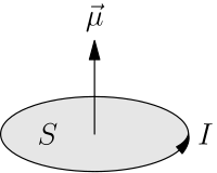
случае плоского контура с электрическим
током магнитный момент вычисляется как

,

где I — сила
тока в
контуре, S —
площадь контура,  —
единичный вектор нормали к плоскости
контура. Направление магнитного момента
обычно находится по правилу
буравчика:
если вращать ручку буравчика в направлении
тока, то направление магнитного момента
будет совпадать с направлением
поступательного движения буравчика.

Для
произвольного замкнутого контура
магнитный момент находится из:

,

где  — радиус-вектор,
проведенный из начала координат до
элемента длины контура 

В
общем случае произвольного распределения
токов в среде:

,

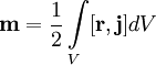где  — плотность
тока в
элементе объёма dV.

8. Принцип суперпозиции

За
положительное направление
векторапринимается
направление от южного полюсаS к
северному полюсу N магнитной
стрелки, свободно ориентирующийся в
магнитном поле. Таким образом, исследуя
магнитное поле, создаваемое током или
постоянным магнитом, с помощью маленькой
магнитной стрелки, можно в каждой точке
пространства определить направление
вектора .

Направление
этого вектора для поля прямого проводника
с током и соленоида можно определить
по правилу буравчика:
если направление поступательного
движения буравчика (винта) с правой
нарезкой совпадает с направлением тока
в проводнике, то направление вращения
ручки буравчика совпадает с направлением
вектора магнитной индукции.

Модуль
индукции B магнитного
поля прямолинейного проводника с
током I на
расстоянии R от
него выражается соотношением:

где
μ₀ –
постоянная величина, которую
называют магнитной
постоянной.
Ее численное значение равно μ₀ =
4π∙10^–7 H/A² ≈
1,26∙10^–6 H/A².

Принцип
суперпозиции магнитных полей:
если магнитное поле создано несколькими
проводниками с токами, то вектор магнитной
индукции в какой-либо точке этого поля
равен векторной сумме магнитных индукций,
созданных в этой точке каждым током в
отдельности:

9. Поток магнитного поля

Магни́тный
пото́к — поток  как
интеграл вектора магнитной
индукции  через
конечную поверхность .
Определяется через интеграл по поверхности

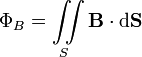
при
этом векторный элемент площади поверхности
определяется как

где  — единичный
вектор, нормальный к
поверхности.

Также
магнитный поток можно рассчитать как
скалярное произведение вектора магнитной
индукции на вектор площади:

где α —
угол между вектором магнитной индукции
и нормалью к
плоскости площади.

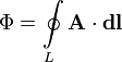
Магнитный
поток через контур также можно выразить
через циркуляцию векторного
потенциала магнитного
поля по этому контуру:

В
системе СИ единицей магнитного
потока является Вебер (Вб, размерность — В·с = кг·м²·с⁻²·А⁻¹),
в системе СГС — максвелл (Мкс);
1 Вб = 10⁸ Мкс.

10. *Момент сил, действующих на контур с током в магнитном поле

Опыт показывает, что моментсил,действующихнаконтур,
зависит от его ориентации в пространстве,
следовательно, физическая величина,
описывающее магнитноеполе,
должна быть векторной. В общем случае
этот вектор может изменяться от точки
к точке, поэтому магнитноеполедолжно
описываться математически как уже
знакомое намвекторной поле.

Так как мы хотим определить «точечную»
характеристику магнитного поля, то
такой контур(или магнитную
стрелку)следует считать бесконечно
малым.

В очередной раз мы должны сделать
традиционную оговорку – бесконечно
малый контурфизически
нереализуем – даже провода имеют
конечную толщину, поэтому переход к
бесконечно малому контуру следует
понимать в физическом смысле – мал,
настолько, что с математической точки
можно считать бесконечно малым, но
реально реализуемым.

Чтобы избавиться от неоднозначности
измеряемого момента сил, связанной
с ориентацией контура, выберем такое
положение контура, при котором модель
моментасилмаксималенM_max.
Наконец, учтем еще один экспериментальный
факт –момент сил, действующих на контур,
пропорционален силе тока в контуре I и
площади контура S.

Следовательно, отношение момента сил к
произведению силы тока в контуре на его
площадь является величиной, не зависящей
от свойств контура, поэтому является
характеристикой поля, которая называется
индукцией магнитного поля

.
(8)

In electromagnetism, the magnetic moment is the magnetic strength and orientation of a magnet or other object that produces a magnetic field. Examples of objects that have magnetic moments include loops of electric current (such as electromagnets), permanent magnets, elementary particles (such as electrons), various molecules, and many astronomical objects (such as many planets, some moons, stars, etc).

More precisely, the term magnetic moment normally refers to a system’s magnetic dipole moment, the component of the magnetic moment that can be represented by an equivalent magnetic dipole: a magnetic north and south pole separated by a very small distance. The magnetic dipole component is sufficient for small enough magnets or for large enough distances. Higher-order terms (such as the magnetic quadrupole moment) may be needed in addition to the dipole moment for extended objects.

The magnetic dipole moment of an object is readily defined in terms of the torque that the object experiences in a given magnetic field. The same applied magnetic field creates larger torques on objects with larger magnetic moments. The strength (and direction) of this torque depends not only on the magnitude of the magnetic moment but also on its orientation relative to the direction of the magnetic field. The magnetic moment may be considered, therefore, to be a vector. The direction of the magnetic moment points from the south to north pole of the magnet (inside the magnet).

The magnetic field of a magnetic dipole is proportional to its magnetic dipole moment. The dipole component of an object’s magnetic field is symmetric about the direction of its magnetic dipole moment, and decreases as the inverse cube of the distance from the object.

Definition, units, and measurement[edit]

Definition[edit]

The magnetic moment can be defined as a vector relating the aligning torque on the object from an externally applied magnetic field to the field vector itself. The relationship is given by:^[1]

where τ is the torque acting on the dipole, B is the external magnetic field, and m is the magnetic moment.

This definition is based on how one could, in principle, measure the magnetic moment of an unknown sample. For a current loop, this definition leads to the magnitude of the magnetic dipole moment equaling the product of the current times the area of the loop. Further, this definition allows the calculation of the expected magnetic moment for any known macroscopic current distribution.

An alternative definition is useful for thermodynamics calculations of the magnetic moment. In this definition, the magnetic dipole moment of a system is the negative gradient of its intrinsic energy, U_int, with respect to external magnetic field:

Generically, the intrinsic energy includes the self-field energy of the system plus the energy of the internal workings of the system. For example, for a hydrogen atom in a 2p state in an external field, the self-field energy is negligible, so the internal energy is essentially the eigenenergy of the 2p state, which includes Coulomb potential energy and the kinetic energy of the electron. The interaction-field energy between the internal dipoles and external fields is not part of this internal energy.^[2]

Units[edit]

The unit for magnetic moment in International System of Units (SI) base units is A⋅m², where A is ampere (SI base unit of current) and m is meter (SI base unit of distance). This unit has equivalents in other SI derived units including:^[3][4]

where N is newton (SI derived unit of force), T is tesla (SI derived unit of magnetic flux density), and J is joule (SI derived unit of energy).^[5] Although torque (N·m) and energy (J) are dimensionally equivalent, torques are never expressed in units of energy.^[6]

In the CGS system, there are several different sets of electromagnetism units, of which the main ones are ESU, Gaussian, and EMU. Among these, there are two alternative (non-equivalent) units of magnetic dipole moment:

(ESU)

(Gaussian and EMU),

where statA is statamperes, cm is centimeters, erg is ergs, and G is gauss. The ratio of these two non-equivalent CGS units (EMU/ESU) is equal to the speed of light in free space, expressed in cm⋅s⁻¹.

All formulae in this article are correct in SI units; they may need to be changed for use in other unit systems. For example, in SI units, a loop of current with current I and area A has magnetic moment IA (see below), but in Gaussian units the magnetic moment is IA/c.

Other units for measuring the magnetic dipole moment include the Bohr magneton and the nuclear magneton.

Measurement[edit]

The magnetic moments of objects are typically measured with devices called magnetometers, though not all magnetometers measure magnetic moment: Some are configured to measure magnetic field instead. If the magnetic field surrounding an object is known well enough, though, then the magnetic moment can be calculated from that magnetic field.

Relation to magnetization[edit]

The magnetic moment is a quantity that describes the magnetic strength of an entire object. Sometimes, though, it is useful or necessary to know how much of the net magnetic moment of the object is produced by a particular portion of that magnet. Therefore, it is useful to define the magnetization field M as:

where m_ΔV and V_ΔV are the magnetic dipole moment and volume of a sufficiently small portion of the magnet ΔV. This equation is often represented using derivative notation such that

where dm is the elementary magnetic moment and dV is the volume element. The net magnetic moment of the magnet m therefore is

where the triple integral denotes integration over the volume of the magnet. For uniform magnetization (where both the magnitude and the direction of M is the same for the entire magnet (such as a straight bar magnet) the last equation simplifies to:

where V is the volume of the bar magnet.

The magnetization is often not listed as a material parameter for commercially available ferromagnetic materials, though. Instead the parameter that is listed is residual flux density (or remanence), denoted B_r. The formula needed in this case to calculate m in (units of A⋅m²) is:

,

where:

• B_r is the residual flux density, expressed in teslas.
• V is the volume of the magnet (in m³).
• μ₀ is the permeability of vacuum (4π×10⁻⁷ H/m).^[7]

Models[edit]

The preferred classical explanation of a magnetic moment has changed over time. Before the 1930s, textbooks explained the moment using hypothetical magnetic point charges. Since then, most have defined it in terms of Ampèrian currents.^[8] In magnetic materials, the cause of the magnetic moment are the spin and orbital angular momentum states of the electrons, and varies depending on whether atoms in one region are aligned with atoms in another.

Magnetic pole model[edit]

The sources of magnetic moments in materials can be represented by poles in analogy to electrostatics. This is sometimes known as the Gilbert model.^[9] In this model, a small magnet is modeled by a pair of fictitious magnetic monopoles of equal magnitude but opposite polarity. Each pole is the source of magnetic force which weakens with distance. Since magnetic poles always come in pairs, their forces partially cancel each other because while one pole pulls, the other repels. This cancellation is greatest when the poles are close to each other i.e. when the bar magnet is short. The magnetic force produced by a bar magnet, at a given point in space, therefore depends on two factors: the strength p of its poles (magnetic pole strength), and the vector separating them. The magnetic dipole moment m is related to the fictitious poles as^[8]

It points in the direction from South to North pole. The analogy with electric dipoles should not be taken too far because magnetic dipoles are associated with angular momentum (see Relation to angular momentum). Nevertheless, magnetic poles are very useful for magnetostatic calculations, particularly in applications to ferromagnets.^[8] Practitioners using the magnetic pole approach generally represent the magnetic field by the irrotational field H, in analogy to the electric field E.

Amperian loop model[edit]

After Hans Christian Ørsted discovered that electric currents produce a magnetic field and André-Marie Ampère discovered that electric currents attract and repel each other similar to magnets, it was natural to hypothesize that all magnetic fields are due to electric current loops. In this model developed by Ampère, the elementary magnetic dipole that makes up all magnets is a sufficiently small amperian loop of current I. The dipole moment of this loop is

where S is the area of the loop. The direction of the magnetic moment is in a direction normal to the area enclosed by the current consistent with the direction of the current using the right hand rule.

Localized current distributions[edit]

The magnetic dipole moment can be calculated for a localized (does not extend to infinity) current distribution assuming that we know all of the currents involved. Conventionally, the derivation starts from a multipole expansion of the vector potential. This leads to the definition of the magnetic dipole moment as:

where × is the vector cross product, r is the position vector, and j is the electric current density and the integral is a volume integral.^[10] When the current density in the integral is replaced by a loop of current I in a plane enclosing an area S then the volume integral becomes a line integral and the resulting dipole moment becomes

which is how the magnetic dipole moment for an Amperian loop is derived.

Practitioners using the current loop model generally represent the magnetic field by the solenoidal field B, analogous to the electrostatic field D.

Magnetic moment of a solenoid[edit]

A generalization of the above current loop is a coil, or solenoid. Its moment is the vector sum of the moments of individual turns. If the solenoid has N identical turns (single-layer winding) and vector area S,

Quantum mechanical model[edit]

When calculating the magnetic moments of materials or molecules on the microscopic level it is often convenient to use a third model for the magnetic moment that exploits the linear relationship between the angular momentum and the magnetic moment of a particle. While this relation is straightforward to develop for macroscopic currents using the amperian loop model (see below), neither the magnetic pole model nor the amperian loop model truly represents what is occurring at the atomic and molecular levels. At that level quantum mechanics must be used. Fortunately, the linear relationship between the magnetic dipole moment of a particle and its angular momentum still holds, although it is different for each particle. Further, care must be used to distinguish between the intrinsic angular momentum (or spin) of the particle and the particle’s orbital angular momentum. See below for more details.

Effects of an external magnetic field[edit]

Torque on a moment[edit]

The torque τ on an object having a magnetic dipole moment m in a uniform magnetic field B is:

.

This is valid for the moment due to any localized current distribution provided that the magnetic field is uniform. For non-uniform B the equation is also valid for the torque about the center of the magnetic dipole provided that the magnetic dipole is small enough.^[11]

An electron, nucleus, or atom placed in a uniform magnetic field will precess with a frequency known as the Larmor frequency. See Resonance.

Force on a moment[edit]

A magnetic moment in an externally produced magnetic field has a potential energy U:

In a case when the external magnetic field is non-uniform, there will be a
force, proportional to the magnetic field gradient, acting on the magnetic moment itself. There are two expressions for the force acting on a magnetic dipole, depending on whether the model used for the dipole is a current loop or two monopoles (analogous to the electric dipole).^[12] The force obtained in the case of a current loop model is

.

Assuming existence of magnetic monopole, the force is modified as follows:

In the case of a pair of monopoles being used (i.e. electric dipole model), the force is

.

And one can be put in terms of the other via the relation

.

In all these expressions m is the dipole and B is the magnetic field at its position. Note that if there are no currents or time-varying electrical fields or magnetic charge, ∇×B = 0, ∇·B = 0 and the two expressions agree.

Relation to Free Energy[edit]

One can relate the magnetic moment of a system to the free energy of that system.^[13] In a uniform magnetic field B, the free energy F can be related to the magnetic moment M of the system as

where S is the entropy of the system and T is the temperature. Therefore, the magnetic moment can also be defined in terms of the free energy of a system as

.

Magnetism[edit]

In addition, an applied magnetic field can change the magnetic moment of the object itself; for example by magnetizing it. This phenomenon is known as magnetism. An applied magnetic field can flip the magnetic dipoles that make up the material causing both paramagnetism and ferromagnetism. Additionally, the magnetic field can affect the currents that create the magnetic fields (such as the atomic orbits) which causes diamagnetism.

Effects on environment[edit]

Magnetic field of a magnetic moment[edit]

Any system possessing a net magnetic dipole moment m will produce a dipolar magnetic field (described below) in the space surrounding the system. While the net magnetic field produced by the system can also have higher-order multipole components, those will drop off with distance more rapidly, so that only the dipole component will dominate the magnetic field of the system at distances far away from it.

The magnetic field of a magnetic dipole depends on the strength and direction of a magnet’s magnetic moment but drops off as the cube of the distance such that:

where is the magnetic field produced by the magnet and is a vector from the center of the magnetic dipole to the location where the magnetic field is measured. The inverse cube nature of this equation is more readily seen by expressing the location vector as the product of its magnitude times the unit vector in its direction () so that:

The equivalent equations for the magnetic -field are the same except for a multiplicative factor of μ₀ = 4π×10⁻⁷ H/m, where μ₀ is known as the vacuum permeability. For example:

Forces between two magnetic dipoles[edit]

As discussed earlier, the force exerted by a dipole loop with moment m₁ on another with moment m₂ is

where B₁ is the magnetic field due to moment m₁. The result of calculating the gradient is^[14][15]

where r̂ is the unit vector pointing from magnet 1 to magnet 2 and r is the distance. An equivalent expression is^[15]

The force acting on m₁ is in the opposite direction.

Torque of one magnetic dipole on another[edit]

The torque of magnet 1 on magnet 2 is

Theory underlying magnetic dipoles[edit]

The magnetic field of any magnet can be modeled by a series of terms for which each term is more complicated (having finer angular detail) than the one before it. The first three terms of that series are called the monopole (represented by an isolated magnetic north or south pole) the dipole (represented by two equal and opposite magnetic poles), and the quadrupole (represented by four poles that together form two equal and opposite dipoles). The magnitude of the magnetic field for each term decreases progressively faster with distance than the previous term, so that at large enough distances the first non-zero term will dominate.

For many magnets the first non-zero term is the magnetic dipole moment. (To date, no isolated magnetic monopoles have been experimentally detected.) A magnetic dipole is the limit of either a current loop or a pair of poles as the dimensions of the source are reduced to zero while keeping the moment constant. As long as these limits only apply to fields far from the sources, they are equivalent. However, the two models give different predictions for the internal field (see below).

Magnetic potentials[edit]

Traditionally, the equations for the magnetic dipole moment (and higher order terms) are derived from theoretical quantities called magnetic potentials^[16] which are simpler to deal with mathematically than the magnetic fields.

In the magnetic pole model, the relevant magnetic field is the demagnetizing field . Since the demagnetizing portion of does not include, by definition, the part of due to free currents, there exists a magnetic scalar potential such that

.

In the amperian loop model, the relevant magnetic field is the magnetic induction . Since magnetic monopoles do not exist, there exists a magnetic vector potential such that

Both of these potentials can be calculated for any arbitrary current distribution (for the amperian loop model) or magnetic charge distribution (for the magnetic charge model) provided that these are limited to a small enough region to give:

where is the current density in the amperian loop model, is the magnetic pole strength density in analogy to the electric charge density that leads to the electric potential, and the integrals are the volume (triple) integrals over the coordinates that make up . The denominators of these equation can be expanded using the multipole expansion to give a series of terms that have larger of power of distances in the denominator. The first nonzero term, therefore, will dominate for large distances. The first non-zero term for the vector potential is:

where is:

where × is the vector cross product, r is the position vector, and j is the electric current density and the integral is a volume integral.

In the magnetic pole perspective, the first non-zero term of the scalar potential is

Here may be represented in terms of the magnetic pole strength density but is more usefully expressed in terms of the magnetization field as:

The same symbol is used for both equations since they produce equivalent results outside of the magnet.

External magnetic field produced by a magnetic dipole moment[edit]

The magnetic flux density for a magnetic dipole in the amperian loop model, therefore, is

Further, the magnetic field strength is

Internal magnetic field of a dipole[edit]

The two models for a dipole (magnetic poles or current loop) give the same predictions for the magnetic field far from the source. However, inside the source region, they give different predictions. The magnetic field between poles (see the figure for Magnetic pole model) is in the opposite direction to the magnetic moment (which points from the negative charge to the positive charge), while inside a current loop it is in the same direction (see the figure to the right). The limits of these fields must also be different as the sources shrink to zero size. This distinction only matters if the dipole limit is used to calculate fields inside a magnetic material.^[8]

If a magnetic dipole is formed by taking a «north pole» and a «south pole», bringing them closer and closer together but keeping the product of magnetic pole charge and distance constant, the limiting field is^[8]

If a magnetic dipole is formed by making a current loop smaller and smaller, but keeping the product of current and area constant, the limiting field is

Unlike the expressions in the previous section, this limit is correct for the internal field of the dipole.^[8][17]

These fields are related by B = μ₀(H + M), where M(r) = mδ(r) is the magnetization.

Relation to angular momentum[edit]

The magnetic moment has a close connection with angular momentum called the gyromagnetic effect. This effect is expressed on a macroscopic scale in the Einstein–de Haas effect, or «rotation by magnetization», and its inverse, the Barnett effect, or «magnetization by rotation».^[1] Further, a torque applied to a relatively isolated magnetic dipole such as an atomic nucleus can cause it to precess (rotate about the axis of the applied field). This phenomenon is used in nuclear magnetic resonance.

Viewing a magnetic dipole as current loop brings out the close connection between magnetic moment and angular momentum. Since the particles creating the current (by rotating around the loop) have charge and mass, both the magnetic moment and the angular momentum increase with the rate of rotation. The ratio of the two is called the gyromagnetic ratio or so that:^[18][19]

where is the angular momentum of the particle or particles that are creating the magnetic moment.

In the amperian loop model, which applies for macroscopic currents, the gyromagnetic ratio is one half of the charge-to-mass ratio. This can be shown as follows. The angular momentum of a moving charged particle is defined as:

where μ is the mass of the particle and v is the particle’s velocity. The angular momentum of the very large number of charged particles that make up a current therefore is:

where ρ is the mass density of the moving particles. By convention the direction of the cross product is given by the right-hand rule.^[20]

This is similar to the magnetic moment created by the very large number of charged particles that make up that current:

where and is the charge density of the moving charged particles.

Comparing the two equations results in:

where is the charge of the particle and is the mass of the particle.

Even though atomic particles cannot be accurately described as orbiting (and spinning) charge distributions of uniform charge-to-mass ratio, this general trend can be observed in the atomic world so that:

where the g-factor depends on the particle and configuration. For example the g-factor for the magnetic moment due to an electron orbiting a nucleus is one while the g-factor for the magnetic moment of electron due to its intrinsic angular momentum (spin) is a little larger than 2. The g-factor of atoms and molecules must account for the orbital and intrinsic moments of its electrons and possibly the intrinsic moment of its nuclei as well.

In the atomic world the angular momentum (spin) of a particle is an integer (or half-integer in the case of spin) multiple of the reduced Planck constant ħ. This is the basis for defining the magnetic moment units of Bohr magneton (assuming charge-to-mass ratio of the electron) and nuclear magneton (assuming charge-to-mass ratio of the proton). See electron magnetic moment and Bohr magneton for more details.

Atoms, molecules, and elementary particles[edit]

Fundamentally, contributions to any system’s magnetic moment may come from sources of two kinds: motion of electric charges, such as electric currents; and the intrinsic magnetism of elementary particles, such as the electron.

Contributions due to the sources of the first kind can be calculated from knowing the distribution of all the electric currents (or, alternatively, of all the electric charges and their velocities) inside the system, by using the formulas below. On the other hand, the magnitude of each elementary particle’s intrinsic magnetic moment is a fixed number, often measured experimentally to a great precision. For example, any electron’s magnetic moment is measured to be −9.284764×10⁻²⁴ J/T.^[21] The direction of the magnetic moment of any elementary particle is entirely determined by the direction of its spin, with the negative value indicating that any electron’s magnetic moment is antiparallel to its spin.

The net magnetic moment of any system is a vector sum of contributions from one or both types of sources.
For example, the magnetic moment of an atom of hydrogen-1 (the lightest hydrogen isotope, consisting of a proton and an electron) is a vector sum of the following contributions:

1. the intrinsic moment of the electron,
2. the orbital motion of the electron around the proton,
3. the intrinsic moment of the proton.

Similarly, the magnetic moment of a bar magnet is the sum of the contributing magnetic moments, which include the intrinsic and orbital magnetic moments of the unpaired electrons of the magnet’s material and the nuclear magnetic moments.

Magnetic moment of an atom[edit]

For an atom, individual electron spins are added to get a total spin, and individual orbital angular momenta are added to get a total orbital angular momentum. These two then are added using angular momentum coupling to get a total angular momentum. For an atom with no nuclear magnetic moment, the magnitude of the atomic dipole moment, , is then^[22]

where j is the total angular momentum quantum number, g_J is the Landé g-factor, and μ_B is the Bohr magneton. The component of this magnetic moment along the direction of the magnetic field is then^[23]

The negative sign occurs because electrons have negative charge.

The integer m (not to be confused with the moment, ) is called the magnetic quantum number or the equatorial quantum number, which can take on any of 2j + 1 values:^[24]

Due to the angular momentum, the dynamics of a magnetic dipole in a magnetic field differs from that of an electric dipole in an electric field. The field does exert a torque on the magnetic dipole tending to align it with the field. However, torque is proportional to rate of change of angular momentum, so precession occurs: the direction of spin changes. This behavior is described by the Landau–Lifshitz–Gilbert equation:^[25][26]

where γ is the gyromagnetic ratio, m is the magnetic moment, λ is the damping coefficient and H_eff is the effective magnetic field (the external field plus any self-induced field). The first term describes precession of the moment about the effective field, while the second is a damping term related to dissipation of energy caused by interaction with the surroundings.

Magnetic moment of an electron[edit]

Electrons and many elementary particles also have intrinsic magnetic moments, an explanation of which requires a quantum mechanical treatment and relates to the intrinsic angular momentum of the particles as discussed in the article Electron magnetic moment. It is these intrinsic magnetic moments that give rise to the macroscopic effects of magnetism, and other phenomena, such as electron paramagnetic resonance.

The magnetic moment of the electron is

where μ_B is the Bohr magneton, S is electron spin, and the g-factor g_S is 2 according to Dirac’s theory, but due to quantum electrodynamic effects it is slightly larger in reality: 2.00231930436. The deviation from 2 is known as the anomalous magnetic dipole moment.

Again it is important to notice that m is a negative constant multiplied by the spin, so the magnetic moment of the electron is antiparallel to the spin. This can be understood with the following classical picture: if we imagine that the spin angular momentum is created by the electron mass spinning around some axis, the electric current that this rotation creates circulates in the opposite direction, because of the negative charge of the electron; such current loops produce a magnetic moment which is antiparallel to the spin. Hence, for a positron (the anti-particle of the electron) the magnetic moment is parallel to its spin.

Magnetic moment of a nucleus[edit]

The nuclear system is a complex physical system consisting of nucleons, i.e., protons and neutrons. The quantum mechanical properties of the nucleons include the spin among others. Since the electromagnetic moments of the nucleus depend on the spin of the individual nucleons, one can look at these properties with measurements of nuclear moments, and more specifically the nuclear magnetic dipole moment.

Most common nuclei exist in their ground state, although nuclei of some isotopes have long-lived excited states. Each energy state of a nucleus of a given isotope is characterized by a well-defined magnetic dipole moment, the magnitude of which is a fixed number, often measured experimentally to a great precision. This number is very sensitive to the individual contributions from nucleons, and a measurement or prediction of its value can reveal important information about the content of the nuclear wave function. There are several theoretical models that predict the value of the magnetic dipole moment and a number of experimental techniques aiming to carry out measurements in nuclei along the nuclear chart.

Magnetic moment of a molecule[edit]

Any molecule has a well-defined magnitude of magnetic moment, which may depend on the molecule’s energy state. Typically, the overall magnetic moment of a molecule is a combination of the following contributions, in the order of their typical strength:

• magnetic moments due to its unpaired electron spins (paramagnetic contribution), if any
• orbital motion of its electrons, which in the ground state is often proportional to the external magnetic field (diamagnetic contribution)
• the combined magnetic moment of its nuclear spins, which depends on the nuclear spin configuration.

Examples of molecular magnetism[edit]

• The dioxygen molecule, O₂, exhibits strong paramagnetism, due to unpaired spins of its outermost two electrons.
• The carbon dioxide molecule, CO₂, mostly exhibits diamagnetism, a much weaker magnetic moment of the electron orbitals that is proportional to the external magnetic field. The nuclear magnetism of a magnetic isotope such as ¹³C or ¹⁷O will contribute to the molecule’s magnetic moment.
• The dihydrogen molecule, H₂, in a weak (or zero) magnetic field exhibits nuclear magnetism, and can be in a para- or an ortho- nuclear spin configuration.
• Many transition metal complexes are magnetic. The spin-only formula is a good first approximation for high-spin complexes of first-row transition metals.^[27]

Number of unpaired electrons	Spin-only moment (μB)
1	1.73
2	2.83
3	3.87
4	4.90
5	5.92

Elementary particles[edit]

In atomic and nuclear physics, the Greek symbol μ represents the magnitude of the magnetic moment, often measured in Bohr magnetons or nuclear magnetons, associated with the intrinsic spin of the particle and/or with the orbital motion of the particle in a system. Values of the intrinsic magnetic moments of some particles are given in the table below:

Intrinsic magnetic moments and spins
of some elementary particles^[28]

Particle name (symbol)	Magnetic dipole moment (10−27 J⋅T−1)	Spin quantum number (dimensionless)
electron (e−)	−9284.764	1/2
proton (H+)	–0 014.106067	1/2
neutron (n)	0 00−9.66236	1/2
muon (μ−)	0 0−44.904478	1/2
deuteron (2H+)	–0 004.3307346	1
triton (3H+)	–0 015.046094	1/2
helion (3He++)	0 0−10.746174	1/2
alpha particle (4He++)	–0 000	0

For the relation between the notions of magnetic moment and magnetization see magnetization.

See also[edit]

• Moment (physics)
• Electric dipole moment
• Toroidal dipole moment
• Magnetic susceptibility
• Orbital magnetization
• Magnetic dipole–dipole interaction
• Electron magnetic moment
• Nucleon magnetic moment

References and notes[edit]

External links[edit]

• Bowtell, Richard (2009). «μ – Magnetic Moment». Sixty Symbols. Brady Haran for the University of Nottingham.

Физическая величина; измеряется в ампер-квадратном метре

. Магнитный момент — это сила магнитного поля и ориентация магнита или другого объекта, который создает магнитное поле. Примеры объектов, обладающих магнитными моментами, включают: контуры электрического тока (например, электромагниты ), постоянные магниты, движущиеся элементарные частицы (такие как электроны ), различные молекулы и многие астрономические объекты (например, многие планеты, луны, звезды и т. Д.).

Точнее, термин «магнитный момент» обычно относится к магнитному дипольному моменту системы, который может быть представлен эквивалентным магнитным диполем : магнитный северный и южный полюсы, разделенные очень короткие расстояния длины. Компонента магнитного диполя достаточно для достаточно маленьких магнитов или для достаточно больших расстояний. Члены более высокого порядка (такие как магнитный квадрупольный момент ) могут потребоваться в дополнение к дипольному моменту для протяженных объектов.

Магнитный дипольный момент объекта легко определить в терминах крутящего момента, объект испытывает в данном магнитном поле. То же приложенное магнитное поле создает большие крутящие моменты на объектх с большими магнитными моментами. Сила (и направление) этого крутящего зависит не только от величины магнитного момента, но и от его ориентации относительно направления магнитного поля. Следовательно, магнитный момент можно рассматривать как вектор . Направление магнитного момента указывает с юга на северный полюс магнита (внутри магнита).

Магнитное поле магнитного диполя пропорционально его магнитному дипольному моменту. Дипольная составляющая магнитного поля объекта симметрична относительно направления его магнитного дипольного момента и уменьшается как куб, обратный расстояния от объекта.

Содержание

• 1 Определение, единицы и измерение
  • 1.1 Определение
  • 1.2 Единицы
  • 1.3 Измерение
• 2 Отношение к намагничиванию
• 3 Модели
  • 3.1 Модель магнитного полюса
  • 3.2 Модель петли Ампера
    • 3.2.1 Локализованные распределения тока
    • 3.2.2 Магнитный момент соленоида
  • 3.3 Квантовая механическая модель
• 4 Влияние внешнего магнитного поля
  • 4.1 Крутящий момент на момент
  • 4.2 Сила, действующая в момент
  • 4.3 Магнетизм
• 5 Воздействие на среду среды
  • 5.1 Магнитное поле магнитного момента
  • 5.2 Силы между двумя магнитными диполями
  • 5.3 Крутящий момент одного магнитного диполя на другой
• 6 Теория, лежащая в основе магнитных диполей
  • 6.1 Магнитные потенциалы
  • 6.2 Внешнее магнитное поле, создаваемое магнитным дипольным моментом
  • 6.3 Внутреннее магнитное поле диполя
• 7 Отношение к угловому моменту
• 8 Атомов, молекулы и элементарные частицы
  • 8.1 Магнитный момент атома
  • 8.2 Магнитный моменте нт электрона
  • 8.3 Магнитный момент ядра
  • 8.4 Магнитный м элемент молекулы
    • 8.4.1 Примеры молекулярного магнетизма
  • 8.5 Элементарные частицы
• 9 См. также
• 10 Ссылки и примечания
• 11 Внешние ссылки

Определение, единицы и измерения

Определение

Магнитный момент может быть определен как вектор, связывающий выравнивающий крутящий момент на объекте от приложенного извне магнитного поля к самому вектору поля. Отношение задается следующим образом:

τ = m × B { displaystyle { boldsymbol { tau}} = mathbf {m} times mathbf {B}}

где τ — крутящий момент, действующий на диполь, B — внешнее магнитное поле, а m — магнитный момент.

Это определение основано на том, как можно в принципе измерить магнитный момент неизвестного образца. Для токовой петли это определение приводит к тому, что величина магнитного дипольного момента равна произведению тока на площади петли. Кроме того, это определение позволяет рассчитать ожидаемый магнитный момент для любого известного макроскопического распределения тока.

Альтернативное определение полезно для термодинамических расчетов магнитного момента. В этом определении магнитный дипольный момент — это отрицательный градиент ее внутренней энергии U int по отношению к внешнему магнитному полю:

m = — x ^ ∂ U int ∂ B x — y ^ ∂ U int ∂ B y — z ^ ∂ U int ∂ B z. { displaystyle mathbf {m} = — { hat { mathbf {x}}} { frac { partial U _ { rm {int}}} { partial B_ {x}}} — { hat { mathbf {y}}} { frac { partial U _ { rm {int}}} { partial B_ {y}}} — { hat { mathbf {z}}} { frac { partial U_ { rm {int}}} { partial B_ {z}}}.}

Как правило, собственная энергия включает в себя энергию собственной поля системы плюс энергия внутренней работы системы. Например, для атома водорода в состоянии 2p во внешнем поле энергии собственного поля пренебрежимо мала, поэтому внутренняя энергия по собственной энергии состояния 2p, которая включает кулоновскую потенциальную энергию и кинетическую энергию электрона. Энергия поля взаимодействия между внутренними диполями и внешними полями не является частью этой внутренней энергии.

Единицы

Единицы измерения магнитного момента в Международной системе единиц (СИ) базовые единицы — А isм, где А — ампер (базовая единица измерения тока в системе СИ), а м — метр (базовая единица измерения тока в системе СИ). Эта единица имеет эквиваленты в других производных единицах СИ, включая:

A ⋅ m 2 = N ⋅ m T = JT, { displaystyle { text {A}} { cdot} { text {m}} ^ { 2} = { frac {{ text {N}} { cdot} { text {m}}} { text {T}}} = { frac { text {J}} { text {T }}},}

где N — ньютон (производная единица силы в системе СИ), T — тесла (производная единица плотности магнитного потока в системе СИ), а Дж — джоуль (производная единица СИ для энергии ). Хотя крутящий момент (Н · м) и энергия (Дж) эквивалентны по размерам, крутящие моменты никогда не выражаются в единицах энергии.

В системе CGS существует несколько различных наборов единиц электромагнетизма., из которых используются ESU, Gaussian и EMU. Среди них есть две альтернативные (неэквивалентные) единицы магнитного дипольного момента:

1 статА ⋅ см 2 = 3,33564095 × 10-14 А ⋅ м 2 { displaystyle 1 { text {statA}} { cdot} { текст {cm}} ^ {2} = 3,33564095 times 10 ^ {- 14} { text {A}} { cdot} { text {m}} ^ {2}}(ESU)

1 эрг G = 10 — 3 A ⋅ м 2 { displaystyle 1 ; { frac { text {erg}} { text {G}}} = 10 ^ {- 3} { text {A}} { cdot} { text {m}} ^ {2}}(по Гауссу и EMU),

где statA — статамперы, см — сантиметры, эрг составляет эрг, а G составляет гаусс. Отношение этих неэквивалентных единиц CGS (EMU / ESU) равно скорости света в свободном пространстве, выраженной в cm ⋅s.

Все формулы в этой статье верны в SI единиц; их может потребовать изменить для использования в других системах Например, в единицах СИ контур тока с током I и областью A имеет магнитный момент IA (см. Ниже), но в гауссовых единицах магнитный момент равен IA / c.

Другие единицы измерения Магнитный дипольный момент включает магнетон Бора и ядерный магнетон.

Измерение

Магнитные моменты обычно измеряются с помощью устройств, называемых магнитометрами, хотя не все магнитометры измеряют магнитный момент: некоторые из сконфигурированы для измерения магнитного поля вместо этого. Однако, если магнитное поле, окружающее объект, хорошо хорошо, то магнитный момент можно рассчитать на основе этого магнитного поля.

Отношение к намагниченности

Магнитный момент — это величина, которая представляет собой магнитную силу всего объекта. Тем не менее, иногда полезно или необходимо знать, какая часть чистого магнитного момента создается специально этого магнита. Поэтому полезно определить поле намагничивания M { displaystyle mathbf {M}}как:

M = m Δ VV Δ V, { displaystyle mathbf {M} = { frac { mathbf {m} _ { Delta V}} {V _ { Delta V}}},}

где m Δ V { displaystyle mathbf {m} _ { Delta V}}и V Δ V { displaystyle V _ { Delta V}}— магнитный дипольный момент и объем достаточно малой части магнита Δ V { Displaystyle Delta V }. Это уравнение часто представляется с использованием производной записи, такой как

M = dmd V, { displaystyle mathbf {M} = { frac { mathrm {d} mathbf {m}} { mathrm {d} V }},}

где d m — элементарный магнитный момент, а dV — элемент объема. Чистый магнитный момент магнита m { displaystyle mathbf {m}}, следовательно, равенство

m = ∭ M d V, { displaystyle mathbf {m} = iiint mathbf {M} , mathrm {d} V,}

где тройной интеграл обозначает интегрирование по объему магнита. Для однородного намагничивания (где величина и направление M { displaystyle mathbf {M}}одинаковы для всего магнита (например, для прямого стержневого магнита) последнее уравнение упрощает на:

m = MV, { displaystyle mathbf {m} = mathbf {M} V,}

где V { displaystyle V}— объем стержневой магнит.

Однако намагниченность не указывается в качестве материала для ферромагнитных материалов в продаже вместо этого параметра указывается остаточная магнитная индукция (или намагниченность), обозначается B r { displaystyle textstyle mathbf {B} _ {r}}. Формула, необходимая в этом случае для вычислений m { displaystyle mathbf {m}}дюйм (ед. Am) :

m = 1 μ 0 B r V { displaystyle mathbf {m} = { frac {1} { mu _ {0}}} mathbf {B} _ {r} V},

где:

Модели

Предпочтительное классическое объяснение магнитного момента имеет изменилось со временем. До 1930-х годов в учебниках этот момент объяснялся с помощью гипотетических точечных магнитных зарядов. С тех пор большинство определили его в терминах амперских токов. В магнитных материалах причиной магнитного момента наступления состояния спина и орбитального углового момента электронов, и он изменен в зависимости от того, выровнены ли атомы в одной области с атомами в другой.

Модель магнитного полюса

Электростатический аналог магнитного момента: два противоположных заряда, разделенных конечным расстоянием.

Источники магнитных моментов в материалах могут быть представлены полюсами по аналогии с электростатика. Иногда это называют моделью Гилберта. В этой модели магнит моделируется парой магнитных полюсов равной величины, но противоположной полярности . Каждый полюс является магнитной силой, которая ослабевает с расстояниями. Всегда магнитные полюса всегда идут парами, их силы частично компенсируют друг друга, потому что пока один полюс тянет, другой отталкивается. Эта компенсация наиболее велика, когда полюса расположено друг к другу, т.е. когда стержневой магнит короткий. Магнитная сила, создаваемая стержневым магнитом в данной точке пространства, поэтому зависит от двух факторов: силы его полюсов (силы магнитного полюса) и движения ℓ { displaystyle mathrm { boldsymbol { ell}}}разделяя их. Магнитный дипольный момент m связан с фиктивными полюсами как

m = p ℓ. { displaystyle mathbf {m} = p , mathrm { boldsymbol { ell}} ,.}

Он указывает направление с юга на северный полюс. Аналогию с электрическими диполями не следует заходить слишком далеко, поскольку магнитные диполи связаны с угловым моментом (см. Отношение к угловому моменту). Тем не менее, магнитные полюса очень полезны для магнитостатических вычислений, особенно в приложениях к ферромагнетикам. Практики, использующие метод магнитного полюса, обычно используют магнитное поле посредством безвихревого поля H, по аналогии с электрическим полем E.

моделью петли Ампера.

Модель петли Ампера: текущая петля (кольцо), которая переходит на страницу в точке x и выходит в точку, создается поле B (линия). Северный полюс находится справа, а юг — слева.

После Ганс Кристиан Эрстед обнаружил, что электрические токи показывают магнитное поле, а Андре-Мари Ампер обнаружил, что электрические токи притягиваются и отталкиваются друг от друга аналог магнитам, было предположить, что все магнитные поля возникают из-за контуров электрического тока. В этой модели, разработанной Ампером, элементарный магнитный диполь, из которого состоят все магниты, представляет собой достаточно маленькую амперовскую петлю тока I. Дипольный момент этой петли равен

m = IS, { displaystyle mathbf {m} = I { boldsymbol {S}},}

где S — площадь петли. Направление магнитного момента — это направление, нормальное к области, окружающей среде, в соответствии с направлением тока с правилами правой руки.

Локализованные распределения тока

Момент

μ { displaystyle { boldsymbol { mu}}}

плоского тока, имеющего значение I и включающего область S

Магнитный дипольный момент может быть рассчитан для локализованного (не простирающегося до бесконечности) распределения тока, предполагая, что мы знаем все задействованные токи. Обычно вывод начинается с мультипольного разложения потенциально возможной . Это приводит к определению магнитного дипольного момента как:

m = 1 2 ∭ V r × jd V, { displaystyle mathbf {m} = { tfrac {1} {2}} iiint _ {V} mathbf {r} times mathbf {j} , { rm {d}} V,}

где × — Новое рождественское произведение ,, r- вектор положения, а j — это плотность электрического тока, а интеграл — это объемный интеграл. Когда плотность тока в интеграле заменяется петлей тока I в покрывающей области S, тогда объемный интеграл становится линейным интегралом, и результирующий дипольный момент становится

m = IS, { displaystyle mathbf {m} = I mathbf {S},}

— вот как найден магнитный дипольный момент для петли Ампера.

Практики, использующие модель токовой петли, обычно используют магнитное поле с помощью соленоидального поля B, аналогичного электростатического полюса D.

Магнитный момент соленоида

Изображение соленоида

Обобщением вышеупомянутой токовой петли является катушка или соленоид. Его момент — это сумма моментов отдельных поворотов. Если у соленоида N одинаковых витков (однослойная обмотка) и площадь S,

m = NI S. { displaystyle mathbf {m} = NI mathbf {S}.}

Квантовая механическая модель

При вычислении магнитных моментов материалов или молекул на микроскопическом уровне часто бывает удобно использовать третью модель магнитного момента, которая использует линейную зависимость между угловым моментом и магнитным моментом частиц. Хотя это соотношение легко развить для макроскопических токов с использованием моделей ампериановой петли (см. ниже), ни модель магнитного полюса, ни модель амперианской петли в действительности не представляет, что происходит на атомном и молекулярном уровнях. На этом уровне квантовая механика должна познакомиться. К счастью, линейная зависимость между магнитным дипольным моментом частиц и ее угловым моментом все еще сохраняется; хотя для каждой частицы он разный. Кроме того, необходимо соблюдать осторожность, чтобы выделить собственный угловой момент (или спин ) частицы и орбитальный угловой момент частицы. Подробнее см. ниже.

Воздействие внешнего магнитного поля

Крутящий момент на момент

Крутящий момент τ { displaystyle { boldsymbol { tau}}}на объекте, имеющем магнитный дипольный момент m { displaystyle mathbf {m}}в однородном магнитном поле B { displaystyle mathbf {B}}это :

τ = m × B { displaystyle { boldsymbol { tau}} = mathbf {m} times mathbf {B}}.

Это действительно на данный момент из-за любых локализованное распределение тока при условии однородности магнитного поля. Для неоднородного B уравнение также справедливо для крутящего момента вокруг магнитного диполя при условии, что магнитный диполь достаточно мал.

Электрон, ядро ​​или атом, помещенные в однородное магнитное поле, будут прецессировать с размером, известной как частота Лармора. См. Резонанс.

Сила на момент

Магнитный момент во внешнем магнитном поле имеет потенциальную энергию U:

U = — m ⋅ B { displaystyle U = — mathbf {m} cdot mathbf {B}}

В случае, когда внешнее магнитное поле неоднородно, будет сила, пропорциональная магнитному полю градиент, действующая на магнитное поле. сам момент. Есть два выражения для силы, действующая на магнитный диполь, в зависимости от того, является ли модель , используемая для диполя, токовой петлей или двумя монополями (аналогично электрическому диполю). Сила, полученная в случае модели токовой петли, равна

F loop = ∇ (m ⋅ B) { displaystyle mathbf {F} _ { text {loop}} = nabla left ( mathbf {m} cdot mathbf {B} right)}.

В случае использования пары монополей (т.е. модели электрического диполя) сила равна

F диполь = (m ⋅ ∇) B { displaystyle mathbf {F} _ { text {диполь}} = left ( mathbf {m} cdot nabla right) mathbf {B}}.

И одно можно выразить через отношение

F петля = F диполь + m × ( ∇ × B) { displaystyle mathbf {F} _ { text {loop}} = mathbf {F} _ { text {диполь}} + mathbf {m} times left ( nabla times mathbf {B} right)}.

Во всех этих выражениях m — диполь, а B — магнитное поле на своем месте. Обратите внимание, что при отсутствии токов или изменяющихся во времени электрических полей ∇ × B = 0 и два выражения согласуются.

Магнетизм

Кроме того, приложенное магнитное поле может магнитный момент самого объекта; например, намагничивая его. Это явление известно как магнетизм. Приложенное магнитное поле может перевернуть магнитные диполи, из которых состоит материал, вызывая как парамагнетизм, так и ферромагнетизм. Кроме того, магнитное поле может влиять на токи, которые создают магнитные поля (например, атомные орбиты), что вызывает диамагнетизм.

Воздействие на окружающую среду

Магнитное поле магнитного момента

Магнитное поле линии вокруг «магнитостатического диполя». Сам магнитный диполь расположен в центре рисунка, если смотреть сбоку, и направлен вверх.

Любая система, обладающая суммарным магнитным дипольным моментом м, создаст диполь магнитное поле (описанное ниже) в пространстве, окружающем систему. В то время как чистое магнитное поле, создаваемое системой, также может иметь мультипольные компоненты более высокого порядка, они будут убывать с расстоянием быстрее, так что только дипольная компонента будет доминировать в магнитном поле системы на больших расстояниях. подальше от него.

Магнитное поле магнитного диполя зависит от силы и направления магнитного момента магнита m { displaystyle mathbf {m}}, но спадает как куб расстояние такое, что:

H (r) = 1 4 π (3 r (m ⋅ r) | r | 5 -м | г | 3), { displaystyle { mathbf {H}} ({ mathbf {r}}) = { frac {1} {4 pi}} left ({ frac {3 mathbf {r} ( mathbf {m} cdot mathbf {r})} {| mathbf {r} | ^ {5}}} — { frac { mathbf {m}} {| mathbf {r} | ^ {3} }} right),}

где H { displaystyle mathbf {H}}— это магнитное поле, создаваемое магнитом, а r { displaystyle mathbf {r}}— вектор от центра магнитного диполя до места измерения магнитного поля. Обратный кубический характер этого легче увидеть, если выразить вектор местоположения r { displaystyle mathbf {r}}как произведение его величины на единичный вектор в его направлении (r = | r | r ^ { displaystyle mathbf {r} = | mathbf {r} | mathbf { hat {r}}}) так, чтобы:

H (г) = 1 4 π 3 г ^ (г ^ ⋅ м) — м | г | 3. { displaystyle mathbf {H} ( mathbf {r}) = { frac {1} {4 pi}} { frac {3 mathbf { hat {r}} ( mathbf { hat {r}} cdot mathbf {m}) — mathbf {m}} {| mathbf {r} | ^ {3}}}.}

Эквивалентные уравнения для магнитного B { displaystyle mathbf {B}}— те же самые, за исключением мультипликативного коэффициента μ 0 = 4π × 10 H /m, где μ 0 известен как вакуумная проницаемость. Например:

B (r) = μ 0 4 π 3 r ^ (r ^ ⋅ m) — m | г | 3. { displaystyle mathbf {B} ( mathbf {r}) = { frac { mu _ {0}} {4 pi}} { frac {3 mathbf { hat {r}} ( mathbf { hat {r}} cdot mathbf {m}) — mathbf {m}} {| mathbf {r} | ^ {3}}}.}

Силы между двумя магнитными диполями

Как обсуждалось ранее, сила прилагаемой дипольной петлей с моментом m1к другому с моментом m2, равна

F = ∇ (м 2 ⋅ В 1), { displaystyle mathbf {F} = nabla left ( mathbf {m} _ {2} cdot mathbf {B} _ {1} right),}

где B1- магнитное поле, создаваемое моментом m1. Результат вычисления градиента:

F (r, m 1, m 2) = 3 μ 0 4 π | г | 4 (м 2 (м 1 ⋅ г ^) + м 1 (м 2 ⋅ г ^) + г ^ (м 1 ⋅ м 2) — 5 г ^ (м 1 ⋅ г ^) (м 2 ⋅ г ^)), { displaystyle mathbf {F} ( mathbf {r}, mathbf {m} _ {1}, mathbf {m} _ {2}) = { frac {3 mu _ {0}} { 4 пи | mathbf {r} | ^ {4}}} left ( mathbf {m} _ {2} ( mathbf {m} _ {1} cdot { hat { mathbf {r}})}) + mathbf {m} _ {1} ( mathbf {m} _ {2} cdot { hat { mathbf {r}}}) + { hat { mathbf {r}}} ( mathbf {m} _ {1} cdot mathbf {m} _ {2}) — 5 { hat { mathbf {r}}} ( mathbf {m} _ {1} cdot { hat { mathbf {r}}}) ( mathbf {m} _ {2} cdot { hat { mathbf {r}}}) right),}

где r̂ — единица измерения вектора, указывающий от магнита 1 к магниту 2, а r — расстояние. Эквивалентное выражение:

F = 3 μ 0 4 π | г | 4 ((r ^ × m 1) × m 2 + (r ^ × m 2) × m 1 — 2 r ^ (m 1 ⋅ m 2) + 5 r ^ (r ^ × m 1) ⋅ (r ^ × м 2)). { displaystyle mathbf {F} = { frac {3 mu _ {0}} {4 pi | mathbf {r} | ^ {4}}} left (({ hat { mathbf {r}}} times mathbf {m} _ {1}) times mathbf {m} _ {2} + ({ hat { mathbf {r}}} times mathbf {m} _ {2}) times mathbf {m} _ {1} -2 { hat { mathbf {r}}} ( mathbf {m} _ {1} cdot mathbf {m} _ {2}) + 5 { hat { mathbf {r}}} ({ hat { mathbf {r}}} times mathbf {m} _ {1 }) cdot ({ hat { mathbf {r}}} times mathbf {m} _ {2}) right).}

Сила, действующая на m1, имеет противоположное направление.

Крутящий момент одного магнитного диполя на другом

Крутящий момент магнита 1 на магните 2 составляет

τ = м 2 × B 1. { displaystyle { boldsymbol { tau}} = mathbf {m} _ {2} times mathbf {B} _ {1}.}

Теория, лежащая в основе магнитных диполей

Магнитное поле любого магнита можно смоделировать серией членов, для которых каждый член более сложен (имеет более мелкие угловые детали), чем предыдущий. Первые три члена этой серии называются монополем (представлен представленным северным или южным магнитнымсом), диполем (представлен двумя равными и противоположными магнитными полюсами) и квадруполь (представлен четырьмя) полюсами которые, вместе образуют два равных и противоположных диполя). Величина магнитного поля для каждого члена одного расстояния с помощью прогрессивно первого ненулевого члена будет доминировать.

Для многих магнитов первым ненулевым членом является магнитный дипольный момент. (На сегодняшний день магнитных монополей не было экспериментально обнаружено.) Магнитный диполь — это предел либо токовой петли, либо пары полюсов, размеры источника уменьшаются до нуля при сохранении момента постоянного. Эти ограничения применяются только к полям, удаленным от источников, они эквивалентны. Однако эти две модели дают разные прогнозы для внутреннего поля (см. Ниже).

Магнитные потенциалы

Традиционно уравнения для магнитного дипольного момента (и члены более высокого порядка) выводятся из теоретических величин, называемых магнитными возможностями, которые проще обрабатывать математически. затем магнитные поля.

В модели магнитного полюса соответствующее магнитное поле — это размагничивающее поле H { displaystyle mathbf {H}}. Размагничивающая часть H { displaystyle mathbf {H}}по определению не включает часть H { displaystyle mathbf {H}}из-за свободных токов существует магнитный скалярный потенциал такой, что

H (r) = — ∇ ψ { displaystyle { mathbf {H}} ({ mathbf {r}}) = — nabla psi }.

В модели петли амперов соответствующим магнитным полемом является магнитная индукция B { displaystyle mathbf {B}}. Существует магнитный потенциал, такой что

B (r) = × A. { displaystyle mathbf {B} ({ mathbf {r}}) = nabla times { mathbf {A}}.}

Оба эти возможности могут быть вычислены для любого произвольного распределения тока (для ампериана модель петли) или распределения магнитного заряда (для модели магнитного заряда) при условии, что они ограничены достаточно малой областью, чтобы дать:

A (r, t) = μ 0 4 π ∫ j (r ′) | г — г ‘| d V ′, ψ (r, t) = 1 4 π ∫ ρ (r ′) | г — г ‘| d В ‘, { displaystyle { begin {align} mathbf {A} left ( mathbf {r}, t right) = { frac { mu _ {0}} {4 pi}} int { frac { mathbf {j} left ( mathbf {r} ‘ right)} { left | mathbf {r} — mathbf {r} ‘ right |}} , mathrm {d} V’, \ psi left ( mathbf {r}, t right) = { frac { 1} {4 pi}} int { frac { rho left ( mathbf {r} ‘ right)} { left | mathbf {r} — mathbf {r} ‘ right |}} , mathrm {d} V’, end {align}}}

где j { displaystyle mathbf {j} }— плотность тока в модели амперовской петли, ρ { displaystyle rho}представляет собой плотность напряженности магнитного полюса по аналогии с плотностью электрического заряд, который приводит к электрическому потенциалу, интегралы представляют собой объемные (тройные) интегралы по единицам измерения, которые составляют r ′ { displaystyle mathbf {r} ‘}. Знаменатели этого уравнения могут быть расширены с помощью мультипольного разложения , чтобы получить ряды, которые имеют большие размеры в знаменателе. Следовательно, первый ненулевой член будет доминировать на больших расстояниях. Первый ненулевой член предлагать:

A (r) = μ 0 4 π m × r | г | 3, { displaystyle mathbf {A} ( mathbf {r}) = { frac { mu _ {0}} {4 pi}} { frac { mathbf {m} times mathbf {r }} {| mathbf {r} | ^ {3}}},}

где m { displaystyle mathbf {m}}равно:

m = 1 2 ∭ В р × jd В, { Displaystyle mathbf {m} = { tfrac {1} {2}} iiint _ {V} mathbf {r} times mathbf {j} , { rm {d}} V,}

где × — векторное изображение ,, r- положения, а j — плотность электрического тока, интеграл равен объемный интеграл.

С точки зрения магнитного полюса первый ненулевой член скалярного присутствия равенство

ψ (r) = m ⋅ r 4 π | г | 3. { displaystyle psi ( mathbf {r}) = { frac { mathbf {m} cdot mathbf {r}} {4 pi | mathbf {r} | ^ {3}}}.}

Здесь m { displaystyle mathbf {m}}может быть представлено в терминах плотности напряженности магнитного полюса, но более полезно выразить в терминах поля намагниченности как:

m = ∭ M d V. { displaystyle mathbf {m} = iiint mathbf {M} , mathrm {d} V.}

Тот же символ m { displaystyle mathbf {m}}используется для обоих уравнений, так как они дают эквивалентные результаты вне магнита.

Внешнее магнитное поле, создаваемое магнитным дипольным моментом

Следовательно, плотность магнитного потока для магнитного диполя в модели амперовой петли составляет

B (r) = ∇ × A = μ 0 4 π (3 r (mr) | r | 5 — m | r | 3). { displaystyle mathbf {B} ({ mathbf {r}}) = nabla times { mathbf {A}} = { frac { mu _ {0}} {4 pi}} left ( { frac {3 mathbf {r} ( mathbf {m} cdot mathbf {r})} {| mathbf {r} | ^ {5}}} — { frac { mathbf {m}} {| mathbf {r} | ^ {3}}} right).}

Кроме того, напряженность магнитного поля H { displaystyle mathbf {H}}равно

H (r) = — ∇ ψ = 1 4 π (3 r (m ⋅ r) | r | 5 — m | r | 3). { displaystyle { mathbf {H}} ({ mathbf {r}}) = — nabla psi = { frac {1} {4 pi}} left ({ frac {3 mathbf {r } ( mathbf {m} cdot mathbf {r})} {| mathbf {r} | ^ {5}}} — { frac { mathbf {m}} {| mathbf {r} | ^ {3}}} right).}

Внутреннее магнитное поле диполя

Магнитное поле токовой петли

Две модели диполя (токовая петля и магнитные полюса) дают одинаковые предсказания для магнитного поля далеко от источника. Однако внутри источника они дают разные прогнозы. Магнитное поле между полюсами (см. Рисунок для Определение магнитного полюса ) имеет направление, противоположное магнитному моменту (которое указывает от отрицательного заряда к положительному), в то время как внутри токовой петли оно находится в том же направлении ( см. рисунок справа). Пределы этих полей также должны быть разными, поскольку источники сжимаются до нулевого размера. Это различие имеет значение в том случае, если предел диполя используется для расчета полей внутри магнитного материала.

Если магнитный диполь создается и уменьшается при сохранении постоянства произведения тока и площади, величина предельное поле

B (r) = μ 0 4 π [3 r ^ (r ^ ⋅ m) — м | г | 3 + 8 π 3 м δ (г)]. { displaystyle mathbf {B} ( mathbf {r}) = { frac { mu _ {0}} {4 pi}} left [{ frac {3 mathbf { hat {r}} ( mathbf { hat {r}} cdot mathbf {m}) — mathbf {m}} {| mathbf {r} | ^ {3}}} + { frac {8 pi} {3}} mathbf {m} delta ( mathbf {r}) right].}

В отличие от выражений в предыдущем разделе, в этом разделе предел верен для внутреннего поля диполя.

Если магнитный диполь сформирован путем взятия «северного полюса» и «южного полюса», сближения их все ближе и ближе друг к другу, но при сохранении постоянства заряда магнитного полюса и расстояния постоянным, предельное поле будет

H (r) = 1 4 π [3 r ^ (r ^ ⋅ m) — ì | г | 3 — 4 π 3 м δ (г)]. { displaystyle mathbf {H} ( mathbf {r}) = { frac {1} {4 pi}} left [{ frac {3 mathbf { hat {r}} ( mathbf { шляпа {r}} cdot mathbf {m}) — mathbf {m}} {| mathbf {r} | ^ {3}}} — { frac {4 pi} {3}} mathbf {m} delta ( mathbf {r}) right].}

Эти поля связаны между собой B = μ 0(H+ M), где M(r) = mδ(r) — намагниченность.

Отношение к угловому моменту

Магнитный момент имеет тесную связь с угловой момент называется гиромагнитным эффектом. Этот эффект выражается в макроскопическом масштабе в эффекте Эйнштейна – де Гааза, или «вращении за счет намагничивания», и его обратной величине, эффекте Барнетта, или «намагничивание вращением». Кроме того, крутящий момент, приложенный к относительно изолированному магнитному диполю, такому как атомное ядро ​​, может вызвать его прецессию (вращение вокруг оси приложенного поля). Это явление используется в ядерном магнитном резонансе.

Рассмотрение магнитного диполя как токовой петли выявляет тесную связь между магнитным моментом и угловым моментом. Поскольку частицы, создающие ток (вращаясь вокруг петли), имеют заряд и массу, и магнитный момент, и угловой момент увеличиваются с увеличением скорости вращения. Отношение этих двух величин называется гиромагнитным соотношением или γ { displaystyle gamma}, так что:

m = γ L, { displaystyle mathbf { m} = gamma , mathbf {L},}

где L { displaystyle mathbf {L}}— угловой момент частицы или частиц, которые создают магнитный момент.

В модели амперианской петли, которая применяется для макроскопических токов, гиромагнитное отношение составляет половину отношения заряда к массе . Это можно показать следующим образом. Угловой момент движущейся заряженной частицы определяется как:

L = r × p = μ r × v, { displaystyle mathbf {L} = mathbf {r} times mathbf {p} = mu , mathbf {r} times mathbf {v},}

где μ — это масса частицы, а v — скорость частицы. Следовательно, угловой момент очень большого числа заряженных частиц, составляющих ток, равен:

L = ∭ V r × (ρ v) d V, { displaystyle mathbf {L} = iiint _ {V} , mathbf {r} times ( rho mathbf {v}) , { rm {d}} V ,,}

где ρ — массовая плотность движущегося частицы. Условно направление перекрестного произведения задается правилом правой руки .

Это похоже на магнитный момент, создаваемый очень большим количеством заряженных частиц, составляющих этот ток:

m = 1 2 ∭ В р × (ρ Q v) d V, { displaystyle mathbf {m} = { tfrac {1} {2}} iiint _ {V} , mathbf {r} times ( rho _ {Q} mathbf {v}) , { rm {d}} V ,,}

где j = ρ Q v { displaystyle mathbf {j} = rho _ {Q } mathbf {v}}и ρ Q { displaystyle rho _ {Q}}— плотность заряда движущихся заряженных частиц..

Сравнение двух уравнений приводит к следующему:

m = e 2 μ L, { displaystyle mathbf {m} = { frac {e} {2 mu}} , mathbf {L } ,,}

где e { displaystyle e}— заряд частицы, а μ { displaystyle mu}— масса частицы.

Даже хотя атомные частицы нельзя точно описать как орбитальные (и вращающиеся) распределение заряда с однородным отношением заряда к массе, эту общую тенденцию можно наблюдать в атомном мире так, что:

m = ge 2 мкл, { displaystyle mathbf {m} = g , { frac {e} {2 mu}} , mathbf {L},}

где g-фактор зависит от частиц и конфигурации. Например, g-фактор для магнитного электрона, вращающегося вокруг ядра, равен единице, в то время как g-фактор для магнитного момента электрона, вызванного его собственным угловым моментом (спин ), немного больше, чем 2. g-фактор и молекулы должны использовать его собственные моменты электронов, а также, возможно, собственный момент его ядер.

В атомном мире угловой момент (является спин ) частицы целым числом (или полуцелым числом в случае вращения) кратное приведенной постоянной Планка ħ. Это основа для определения магнитного момента магнетона Бора (при условии отношения заряда к массе электрона ) и ядерного магнетона (при условии отношения заряда к массе протона ). См. магнитный момент электрона и Магнетон Бора для подробностей.

Атомы, молекулы и элементарные частицы

По сути, в магнитный момент системы может происходить из двух источников: движение электрические заряды, например электрические токи ; и собственный магнетизм элементарных частиц, таких как электрон.

. Вклады, обусловленные первым производством, могут быть рассчитаны все электрические токи (альтернативно, все электрические заряды и скорости) внутри системы, используя приведенные ниже формулы. С другой, величина собственного магнитного момента каждой частицы частицы частицы являются фиксированной стороны, измеряемой экспериментально с большой точностью. Например, измеренный магнитный момент любого электрона равен -9,284764 × 10 Дж / Тл. Направление магнитного момента любого элемента частицы полностью определяется направлением ее спина, с отрицательным значением, указывающим, что магнитный момент электрона антипараллелен к его спину.

Чистый магнитный момент любой системы — это сумма вкладов от одного или обоих типов систем. Например, магнитный момент атома водорода-1 (легчайшего изотопа водорода, состоящего из протона и электрона) представляет собой векторную сумму следующих вкладов:

1. собственный момент электрон,
2. орбитальное движение электрона вокруг протона,
3. собственный момент протона.

Аналогичным образом, магнитный момент стержневого магнита равенство вкладывающих магнитных моментов, которые включают собственные орбитальные магнитные моменты неспаренных электронов материала магнита и ядерные магнитные моменты.

Магнитный момент атома

Для атома складываются электронные спины, чтобы получить общий спин, и индивидуальные орбитальные угловые моменты складываются, чтобы получить общий орбитальный угловой момент. Затем эти два суммируются с использованием связи по угловому моменту , чтобы получить общий угловой момент. Для атома без ядерного магнитного момента величина дипольного момента атома m атом { displaystyle { mathfrak {m}} _ { text {atom}}},

м атом знак равно г J μ В J (J + 1) { displaystyle { mathfrak {m}} _ { text {atom}} = g _ { rm {J}} , mu _ { rm {B}} , { sqrt {j , (j + 1) ,}}}

где j — квантовое число полного углового момента , g J — g- фактор Ланда, а μ B — магнетон Бора. Тогда составляющая этого магнитного момента вдоль направления магнитного поля равна

м атом, z = — мг Дж μ B { displaystyle { mathfrak {m}} _ {{ text {atom}}, z} = -m , g _ { rm {J}} , mu _ { rm {B}} ~}.

Отрицательный знак, потому что электроны имеют отрицательный заряд.

целое число m (не путать с моментом, m { displaystyle { mathfrak {m}}}) называется магнитное квантовое число или экваториальное квантовое число, которое может принимать любое из 2j + 1 значений:

— j, — (j — 1), ⋯, — 1, 0, + 1, ⋯, + (J — 1), + J { Displaystyle -j, — (J-1), cdots, -1, 0, +1, cdots, + (j-1), + j ~}.

Из-за углового момента динамика магнитного диполя в магнитном поле отличается от динамики электрического диполя в электрическом поле. Поле действительно оказывает крутящий момент на магнитный диполь, стремясь выровнять его с полем. Однако крутящий момент пропорционален скорости изменения углового момента, поэтому прецессия : изменяется направление вращения. Это поведение описывается уравнением Ландау — Лифшица — Гильберта :

1 γ dmdt = m × H eff — λ γ мм × dmdt { displaystyle { frac {1} { gamma}} { frac {{ rm {d}} mathbf {m}} {{ rm {d}} t}} = mathbf {m} times mathbf {H} _ { text {eff}} — { frac { lambda} { gamma m}} mathbf {m} times { frac {{ rm {d}} mathbf {m}} {{ rm {d}} t}}}

где γ — гиромагнитное отношение ,, m- магнитный момент, λ — коэффициент затухания, а Heff — эффективное магнитное поле (внешнее поле плюс любое самоиндуцированное поле). Первый член представил прецессию вокруг эффективного поля, второй — это демпфирующий член, связанный с диссипацией энергии, вызванной воздействием с окружающей средой.

Магнитный момент электрона

Электроны и многие элементарные частицы также имеют собственные магнитные моменты, объяснение которых требует квантово-механической обработки и относится к внутренним угловой момент описывает, как описано в статье Магнитный момент электрона. Именно эти собственные магнитные моменты вызывают макроскопические эффекты магнетизма и другие явления, такие как электронный парамагнитный резонанс.

Магнитный момент электрона

м · S = — g S μ BS ℏ, { displaystyle mathbf {m} _ { text {S}} = — { frac {g _ { text {S}} mu _ { text {B}} mathbf {S}} { hbar}}, }

где μB — магнетон Бора,, S- электрон спин, а g-фактор gS- 2 согласно теории Дирака, но из-за квантово-электродинамических эффектов в действительности он немного больше: 2,00231930436. Отклонение от 2 известно как аномальный магнитный дипольный момент.

. Снова важно отметить, что m — отрицательная константа, умноженная на спин, поэтому магнитный момент электрона антипараллелен спину. Это можно понять с помощью следующей классической картины: электрический ток, создаваемый этим вращением, циркулирует в противоположном направлении из-за отрицательного заряда электрона. ; такие токовые петли магнитный момент, антипараллельный спину. Следовательно, для позитрона (античастицы электрона) магнитный момент параллелен его спину.

Магнитный момент ядра

Ядерная система — это сложная физическая система, состоящая из нуклонов, то есть протонов и нейтронов. К квантово-механическим свойствам нуклонов, среди прочего, относится к спин. Эти свойства можно рассматривать с помощью ядерных моментов, а точнее ядерного магнитного дипольного момента, зависимости от спина отдельных нуклонов.

Наиболее распространенные ядра существуют в своем основном состоянии, хотя ядра некоторых изотопов имеют долгоживущие возбужденные состояния. Каждое энергетическое состояние ядра данного изотопа характеризуется четко определенным магнитным дипольным моментом, величина которого часто измеряемым экспериментально с большой точностью. Это число очень чувствительно к индивидуальному вкладу нуклонов. Существует несколько теоретических моделей, предсказывающих значение магнитного дипольного момента и ряд экспериментальных методов, направленных на проведение измерений в ядрах по ядерной карте.

Магнитный момент молекулы

Любая молекула имеет четко определенное определение магнитного момента, которая может зависеть от энергетического молекулы. Обычно общий магнитный момент молекулы представляет собой комбинацию следующих вкладов в порядке типичной силы:

• магнитные моменты, обусловленные ее неспаренными электронными спинами (парамагнитными вкладками), если любое
• орбитальное движение его электронов, которое в основном состоянии часто пропорционально внешнему магнитному полюсу (диамагнитный вклад)
• объединенный магнитный момент его ядерных спинов, который зависит от конфигурации ядерных спинов.

Примеры молекулярного магнетизма

• молекула двуокиси кислорода, O 2, проявляет сильный парамагнетизм из-за неспаренных спинов двух крайних электронов.
• Молекула диоксида углерода, CO 2, в основном проявляет диамагнетизм, гораздо более слабый магнитный момент электронных орбиталей, который пропорционален внешнему магнитному полю. Ядерный магнетизм магнитного изотопа, такого как C или O, будет магнитному моменту молекулы.
• Молекула дигидрогена, H 2, в слабом (или нулевом) магнитном поле проявляет ядерный магнетизм и может находиться в пара- или орто- конфигурации ядерного спина.
• Многие переходные металлы комплексы магнитные. Формула только для спина — хорошее приближение для высокоспиновых комплексов переходных металлов первого ряда .

Число. неспаренных. электронов	Только спин. момент. (μB )
1	1,73
2	2,83
3	3,87
4	4,90
5	5,92

Элементарные частицы

В атомной и ядерной физике греческий символ μ представляет звездную часть магнитного момента, измеряемого в магнетонах Бора или ядерных магнетонах, связанных с собственным часто спином частиц и / или с орбитальным движением частиц в системе. Значения собственных магнитных моментов некоторых представленных в таблице ниже:

Собственные магнитные моменты и спины. некоторых элементов твердых частиц

Частица. имя (символ)	Магнитный. дипольный момент. (10 J ⋅T )	Спин. квантовое число. (безразмерный )
электрон (e)	−9284,764	1 / 2
протон (H)	–0 014.106067	1/2
нейтрон (n)	0 00−9.66236	1/2
мюон (μ)	0 0-44.904478	1/2
дейтрон (H)	–0 004.3307346	1
тритон (H)	–0 015.046094	1/2
гелион (He)	0 0−10.746174	1/2
альфа-частица (He)	–0 000	0

Для связи между понятиями магнитного момента и намагниченности см. намагниченность.

См. также

Ссылки и примечания

Внешние ссылки

Часто бывает, что задачу не удается решить из-за того, что под рукой нет нужной формулы. Выводить формулу с  самого начала – дело не самое быстрое, а у нас на счету каждая минута.

Ниже мы собрали вместе основные формулы по теме «Электричество и Магнетизм». Теперь, решая задачи, вы сможете пользоваться этим материалом как справочником, чтобы не терять время на поиски нужной информации.

Ежедневная рассылка с полезной информацией для студентов всех направлений – на нашем телеграм-канале.

Магнетизм: определение

Магнетизм – это взаимодействие движущихся электрических зарядов, происходящее посредством магнитного поля.

Поле – особая форма материи. В рамках стандартной модели существует электрическое, магнитное, электромагнитные поля, поле ядерных сил, гравитационное поле и поле Хиггса. Возможно, есть и другие гипотетические поля, о которых мы пока что можем только догадываться или не догадываться вовсе. Сегодня нас интересует магнитное поле.

Магнитная индукция

Так же, как заряженные тела создают вокруг себя электрическое поле, движущиеся заряженные тела порождают магнитное поле. Магнитное поле не только создается движущимися зарядами (электрическим током), но еще и действует на них. По сути магнитное поле можно обнаружить только по действию на движущиеся заряды. А действует оно на них с силой, называемой силой Ампера, о которой речь пойдет позже.

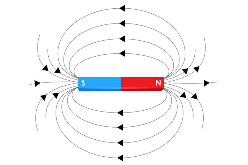
Прежде чем мы начнем приводить конкретные формулы, нужно рассказать про магнитную индукцию.

Магнитная индукция – это силовая векторная характеристика магнитного поля.

Она обозначается буквой B и измеряется в Тесла (Тл). По аналогии с напряженностью для электрического поля Е магнитная индукция показывает, с какой силой магнитное поле действует на заряд.

Кстати, вы найдете много интересных фактов на эту тему в нашей статье про теорию магнитного поля и интересные факты о магнитном поле Земли.

Как определять направление вектора магнитной индукции? Здесь нас интересует практическая сторона вопроса. Самый частый случай в задачах – это магнитное поле, создаваемое проводником с током, который может быть либо прямым, либо в форме окружности или витка.

Для определения направления вектора магнитной индукции существует правило правой руки. Приготовьтесь задействовать абстрактное и пространственное мышление!

Если взять проводник в правую руку так, что большой палец будет указывать на направление тока, то загнутые вокруг проводника пальцы покажут направление силовых линий магнитного поля вокруг проводника. Вектор магнитной индукции в каждой точке будет направлен по касательной к силовым линиям.

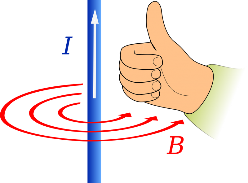
Сила Ампера

Представим, что есть магнитное поле с индукцией B. Если мы поместим в него проводник длиной l, по которому течет ток силой I, то поле будет действовать на проводник с силой:

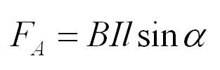
Это и есть сила Ампера. Угол альфа – угол между направлением вектора магнитной индукции и направлением тока в проводнике.

Направление силы Ампера определяется по правилу левой руки: если расположить левую руку так, чтобы в ладонь входили линии магнитной индукции, а вытянутые пальцы указывали бы направление тока, отставленный большой палец укажет направление силы Ампера.

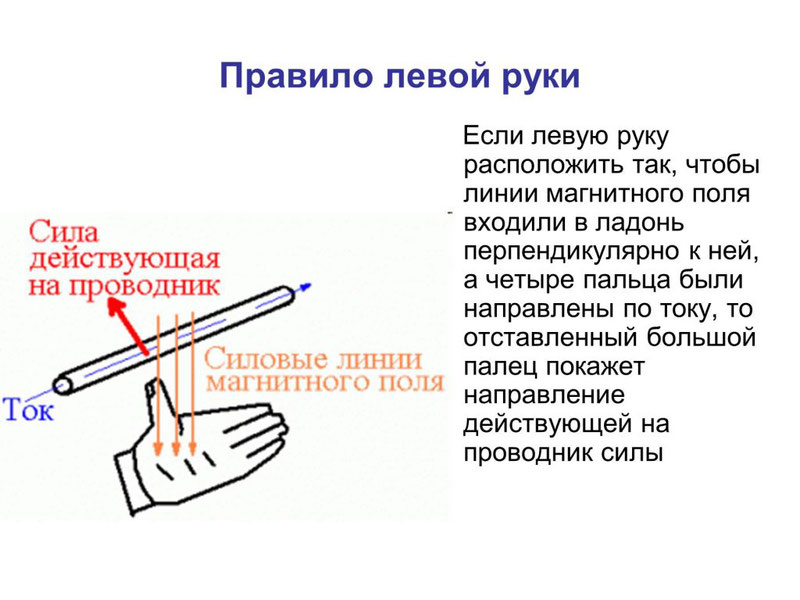
Сила Лоренца

Мы выяснили, что поле действует на проводник с током. Но если это так, то изначально оно действует отдельно на каждый движущийся заряд. Сила, с которой магнитное поле действует на движущийся в нем электрический заряд, называется силой Лоренца. Здесь важно отметить слово «движущийся», так на неподвижные заряды магнитное поле не действует.

Итак, частица с зарядом q движется в магнитном поле с индукцией В со скоростью v, а альфа – это угол между вектором скорости частицы и вектором магнитной индукции. Тогда сила, которая действует на частицу:

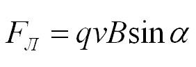
Как определить направление силы Лоренца? По правилу левой руки. Если вектор индукции входит в ладонь, а пальцы указывают на направление скорости, то отогнутый большой палец покажет направление силы Лоренца. Отметим, что так направление определяется для положительно заряженных частиц. Для отрицательных зарядов полученное направление нужно поменять на противоположное.

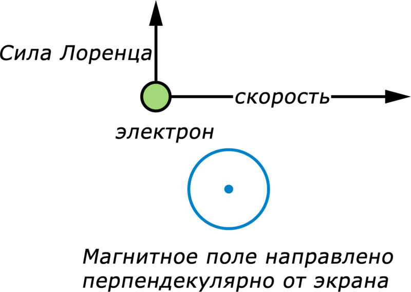
Если частица массы m влетает в поле перпендикулярно линиям индукции, то она будет двигаться по окружности, а сила Лоренца будет играть роль центростремительной силы. Радиус окружности и период обращения частицы в однородном магнитном поле можно найти по формулам:

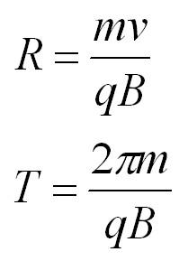
Взаимодействие токов

Рассмотрим два случая. Первый – ток течет по прямому проводу. Второй – по круговому витку. Как мы знаем, ток создает магнитное поле.

В первом случае магнитная индукция провода с током I на расстоянии R от него считается по формуле:

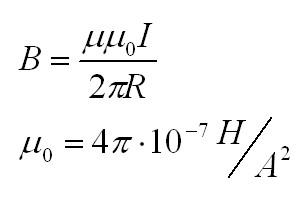
Мю – магнитная проницаемость вещества, мю с индексом ноль – магнитная постоянная.

Во втором случае магнитная индукция в центре кругового витка с током равна:

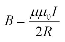
Также при решении задач может пригодиться формула для магнитного поля внутри соленоида. Соленоид – это катушка, то есть множество круговых витков с током.

Пусть их количество – N, а длина самого соленоилда – l. Тогда поле внутри соленоида вычисляется по формуле:

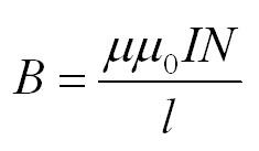
Кстати! Для наших читателей сейчас действует скидка 10% на любой вид работы

Магнитный поток и ЭДС

Если магнитная индукция – векторная характеристика магнитного поля, то магнитный поток – скалярная величина, которая также является одной из самых важных характеристик поля. Представим, что у нас есть какая-то рамка или контур, имеющий определенную площадь. Магнитный поток показывает, какое количество силовых линий проходит через единицу площади, то есть характеризует интенсивность поля. Измеряется в Веберах (Вб) и обозначается Ф.

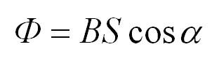
S – площадь контура, альфа – угол между нормалью (перпендикуляром) к плоскости контура и вектором В.

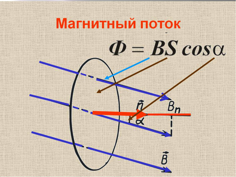
При изменении магнитного потока через контур в контуре индуцируется ЭДС, равная скорости изменения магнитного потока через контур. Кстати, подробнее о том, что такое электродвижущая сила, вы можете почитать в еще одной нашей статье.

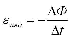
По сути формула выше – это формула для закона электромагнитной индукции Фарадея. Напоминаем, что скорость изменения какой-либо величины есть не что иное, как ее производная по времени.

Для магнитного потока и ЭДС индукции также справедливо обратное. Изменение тока в контуре приводит к изменению магнитного поля и, соответственно, к изменению магнитного потока. При этом возникает ЭДС самоиндукции, которая препятствует изменению тока в контуре. Магнитный поток, который пронизывает контур с током, называется собственным магнитным потоком, пропорционален силе тока в контуре и вычисляется по формуле:

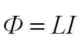
L – коэффициент пропорциональности, называемый индуктивностью, который измеряется в Генри (Гн). На индуктивность влияют форма контура и свойства среды. Для катушки с длиной l и с числом витков N индуктивность рассчитывается по формуле:

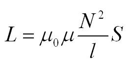
Формула для ЭДС самоиндукции:

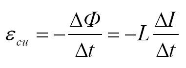
Энергия магнитного поля

Электроэнергия, ядерная энергия, кинетическая энергия. Магнитная энергия – одна из форм энергии. В физических задачах чаще всего нужно рассчитывать энергию магнитного поля катушки. Магнитная энергия катушки с током I и индуктивностью L равна:

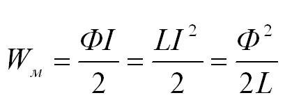
Объемная плотность энергии поля:

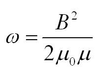
Конечно, это не все основные формулы раздела физики «электричество и магнетизм», однако они часто могут помочь при решении стандартных задач и расчетах. Если же вам попалась задача со звездочкой, и вы никак не можете подобрать к ней ключ, упростите себе жизнь и обратитесь за решением в сервис студенческой помощи.