Содержание:
Нормальный закон распределения:
Нормальный закон распределения имеет плотность вероятности

где 
График функции плотности вероятности (2.9.1) имеет максимум в точке  а точки перегиба отстоят от точки
  на расстояние
  При
При  функция (2.9.1) асимптотически приближается к нулю (ее график изображен на рис. 2.9.1).
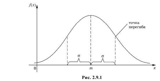
Помимо геометрического смысла, параметры нормального закона распределения имеют и вероятностный смысл. Параметр равен математическому ожиданию нормально распределенной случайной величины, а дисперсия  Если
Если 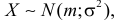 т.е. X имеет нормальный закон распределения с параметрами и
  то
то 
где 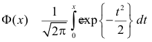 – функция Лапласа
Значения функции  можно найти по таблице (см. прил., табл. П2). Функция Лапласа нечетна, т.е.
 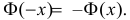 Поэтому ее таблица дана только для неотрицательных
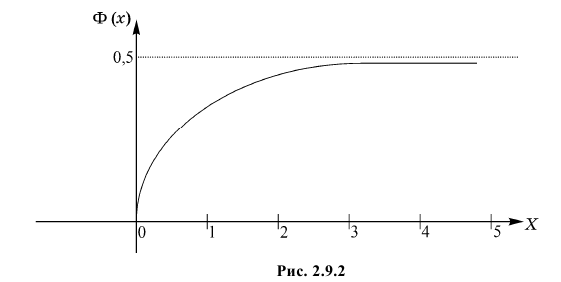
 График функции Лапласа изображен на рис. 2.9.2. При значениях
  она практически остается постоянной. Поэтому в таблице даны значения функции только для
  При значениях можно считать, что
Если 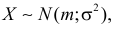 то
то

Пример:
Случайная величина X имеет нормальный закон распределения  Известно, что
  а
а 
 Найти значения параметров
  и
и 
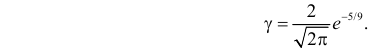
Решение. Воспользуемся формулой (2.9.2): 
Так как  По таблице функции Лапласа (см. прил., табл. П2) находим, что
 Поэтому
  или
или 
Аналогично 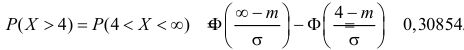 Так как
  то
то  По таблице функции Лапласа (см. прил., табл. П2) находим, что
  Поэтому
  или
или  Из системы двух уравнений
  и
и  находим, что
  а
а  т.е.
т.е.  Итак, случайная величина X имеет нормальный закон распределения N(3;4).
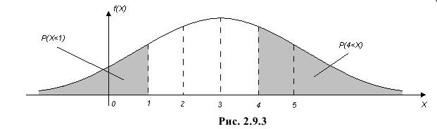
График функции плотности вероятности этого закона распределения изображен на рис. 2.9.3.
Ответ. 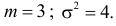
Пример:
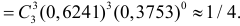
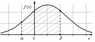
Ошибка измерения X имеет нормальный закон распределения, причем систематическая ошибка равна 1 мк, а дисперсия ошибки равна 4 мк2. Какова вероятность того, что в трех независимых измерениях ошибка ни разу не превзойдет по модулю 2 мк?
Решение. По условиям задачи  Вычислим сначала вероятность того, что в одном измерении ошибка не превзойдет 2 мк. По формуле (2.9.2)
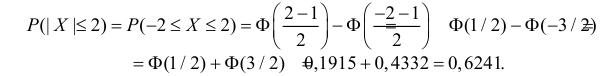
Вычисленная вероятность численно равна заштрихованной площади на рис. 2.9.4.
Каждое измерение можно рассматривать как независимый опыт. Поэтому по формуле Бернулли (2.6.1) вероятность того, что в трех независимых измерениях ошибка ни разу не превзойдет 2 мк, равна 
Ответ. 
Пример:
Функция плотности вероятности случайной величины X имеет вид 
Требуется определить коэффициент  найти
найти  и
и  определить тип закона распределения, нарисовать график функции
  вычислить вероятность
Замечание. Если каждый закон распределения из некоторого семейства законов распределения имеет функцию распределения ,  где
где  – фиксированная функция распределения, a
 то говорят, что эти законы распределения принадлежат к одному виду или типу распределений. Параметр
  называют параметром сдвига,
  – параметром масштаба.
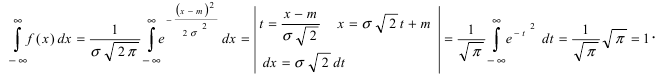
Решение. Так как (2.9.4) функция плотности вероятности, то интеграл от нее по всей числовой оси должен быть равен единице: 
Преобразуем выражение в показателе степени, выделяя полный квадрат: 
Тогда (2.9.5) можно записать в виде 
Сделаем замену переменных так, чтобы  т.е.
т.е. 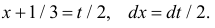 Пределы интегрирования при этом останутся прежними. Тогда (2.9.6) преобразуется к виду
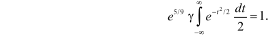
Умножим и разделим левую часть равенства на  Получим равенство
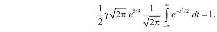
Так как 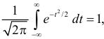 как интеграл по всей числовой оси от функции плотности вероятности стандартного нормального закона распределения N(0,1), то приходим к выводу, что
Поэтому
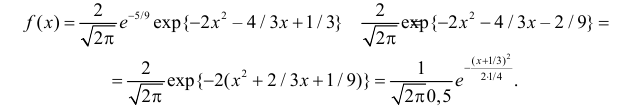
Последняя запись означает, что случайная величина имеет нормальный закон распределения с параметрами  и
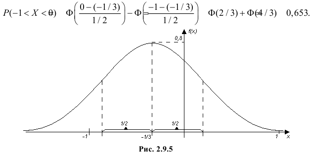
и  График функции плотности вероятности этого закона изображен на рис. 2.9.5. Распределение случайной величины X принадлежит к семейству нормальных законов распределения. По формуле (2.9.2)
Ответ. 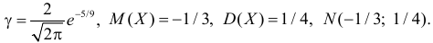
Пример:
Цех на заводе выпускает транзисторы с емкостью коллекторного перехода  Сколько транзисторов попадет в группу
  если в нее попадают транзисторы с емкостью коллекторного перехода от 1,80 до 2,00 пФ. Цех выпустил партию в 1000 штук.
Решение.
Статистическими исследованиями в цеху установлено, что  можно трактовать как случайную величину, подчиняющуюся нормальному закону.
Чтобы вычислить количество транзисторов, попадающих в группу необходимо учитывать, что вся партия транзисторов имеет разброс параметров, накрывающий всю (условно говоря) числовую ось. То есть кривая Гаусса охватывает всю числовую ось, центр ее совпадает с  (т. к. все установки в цеху настроены на выпуск транзисторов именно с этой емкостью). Вероятность попадания отклонений параметров всех транзисторов на всю числовую ось равна 1. Поэтому нам необходимо фактически определить вероятность попадания случайной величины
  в интервал
  а затем пересчитать количество пропорциональной вероятности.
Для расчета этой вероятности надо построить математическую модель. Экспериментальные данные говорят о том, что нормальное распределение можно принять в качестве математической модели. Эмпирическая оценка (установлена статистическими исследованиями в цеху) среднего значения 
дает  оценка среднего квадратического отклонения
Обозначая  подставим приведенные значения в (6.3):
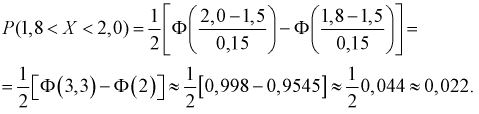
Тогда количество транзисторов  попавших в интервал [1,8; 2,0] пФ, можно найти так:
 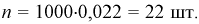 Таким образом можно планировать и рассчитывать количество транзисторов, попадающих в ту или иную группу.
Нормальное распределение и его свойства
Если выйти на улицу любого города и случайным образом выбранных прохожих спросить о том, какой у них рост, вес, возраст, доход, и т.п., а потом построить график любой из этих величин, например, роста… Но не будем спешить, сначала посмотрим, как можно построить такой график.
Сначала, мы просто запишем результаты своего исследования. Потом, мы отсортируем всех людей по группам, так чтобы каждый попал в свой диапазон роста, например, «от 180 до 181 включительно».
После этого мы должны посчитать количество людей в каждой подгруппе-диапазоне, это будет частота попадания роста жителей города в данный диапазон. Обычно эту часть удобно оформить в виде таблички. Если затем эти частоты построить по оси у, а диапазоны отложить по оси х, можно получить так называемую гистограмму, упорядоченный набор столбиков, ширина которых равна, в данном случае, одному сантиметру, а длина будет равна той частоте, которая соответствует каждому диапазону роста. Если
Вам попалось достаточно много жителей, то Ваша схема будет выглядеть примерно так:
Дальше можно уточнить задачу. Каждый диапазон разбить на десять, жителей рассортировать по росту с точностью до миллиметра. Диаграмма станет глаже, но уменьшится по высоте, «оплывет» вниз, т.к. в каждом маленьком диапазоне количество жителей уменьшается. Чтобы избежать этого, просто увеличим масштаб по вертикальной оси в 10 раз. Если гипотетически повторить эту процедуру несколько раз, будет вырисовываться та знаменитая колоколообразная фигура, которая характерна для нормального (или Гауссова) распределения. В результате, относительная частота встречаемости каждого конкретного диапазона роста может быть посчитана как отношение площади «ломтика» кривой, приходящегося на этот диапазон к площади подо всей кривой. Стандартизированные кривые нормального распределения, значения функций которых приводятся в таблицах книг по статистике, всегда имеют суммарную площадь под кривой равную единице. Это связано с тем, что, как Вы помните из курса теории вероятности, вероятность достоверного события всегда равна 100% (или единице), а для любого человека иметь хоть какое-то значение роста — достоверное событие. А вот вероятность того, что рост произвольного человека попадет в определенный выбранный нами диапазон, будет зависеть от трех факторов.
Во-первых, от величины такого диапазона — чем точнее наши требования, тем меньше вероятности, что нам повезет.
Во-вторых, от того, насколько «популярен» выбранный нами рост. Напомним, что мода — самое часто встречающееся значение роста. Кстати для нормального распределения мода, медиана и среднее значение совпадают. Кривая нормального распределения симметрична относительно среднего значения.
И, в-третьих, вероятность попадания роста в определенный диапазон зависит от характеристики рассеивания случайной величины. Отчасти это связано с единицами измерения (представьте, что мы бы измеряли людей в дюймах, а не в миллиметрах, но сами люди и их рост были бы теми же). Но дело не только в этом. Просто некоторые процессы кучнее группируются возле среднего значения, в то время как другие более разбросаны.
Например, рост собак и рост домашних кошек имеют разный разброс значений, их кривые нормального распределения будут выглядеть по-разному (напомним еще раз, что площадь под обеими кривыми будет единичной).
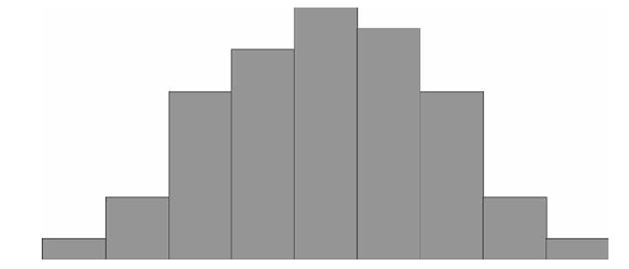
Так, кривая для роста кошек будет более узкой и высокой, а для роста собак кривая будет ниже и шире. Для характеристики разброса конечного ряда данных в прошлом разделе мы использовали величину среднего квадратического отклонения. Аналогичная величина используется для характеристики кривой нормального распределения. Она обозначается буквой s и называется в этом случае стандартным отклонением. Это очень важная величина для кривой нормального распределения. Кривая нормального распределения полностью задана, если известно среднее значение  и отклонение s. Кроме того, любой житель города с вероятностью 68% попадет в диапазон роста
  с вероятностью 95% — в диапазон
 и с вероятностью 99,7% — в диапазон
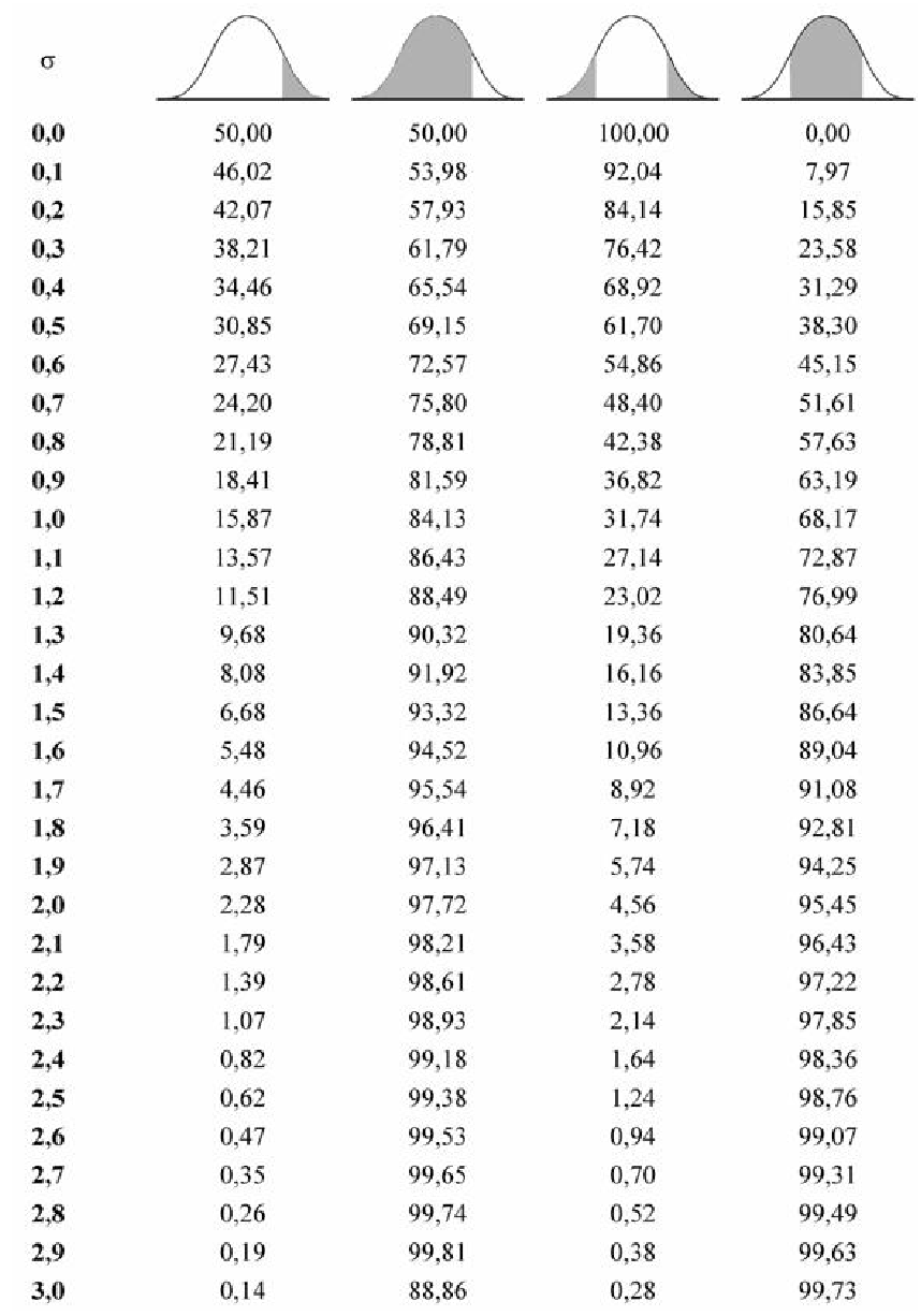
Для вычисления других значений вероятности, которые могут Вам понадобиться, можно воспользоваться приведенной таблицей:
Таблица вероятности попадания случайной величины в отмеченный (заштрихованный) диапазон
Нормальный закон распределения
Нормальный закон распределения случайных величин, который иногда называют законом Гаусса или законом ошибок, занимает особое положение в теории вероятностей, так как 95 % изученных случайных величин подчиняются этому закону. Природа этих случайных величин такова, что их значение в проводимом эксперименте связано с проявлением огромного числа взаимно независимых случайных факторов, действие каждого из которых составляет малую долю их совокупного действия. Например, длина детали, изготавливаемой на станке с программным управлением, зависит от случайных колебаний резца в момент отрезания, от веса и толщины детали, ее формы и температуры, а также от других случайных факторов. По нормальному закону распределения изменяются рост и вес мужчин и женщин, дальность выстрела из орудия, ошибки различных измерений и другие случайные величины.
Определение: Случайная величина X называется нормальной, если она подчиняется нормальному закону распределения, т.е. ее плотность распределения задается формулой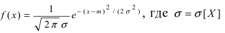 — средне-квадратичное отклонение, a m = М[Х] — математическое ожидание.
Приведенная дифференциальная функция распределения удовлетворяет всем свойствам плотности вероятности, проверим, например, свойство 4.:
Выясним геометрический смысл параметров  Зафиксируем параметр
  и будем изменять параметр m. Построим графики соответствующих кривых (Рис. 8).
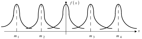
Рис. 8. Изменение графика плотности вероятности в зависимости от изменения математического ожидания при фиксированном значении средне-квадратичного отклонения. Из рисунка видно, кривая  получается путем смещения кривой
  вдоль оси абсцисс на величину m, поэтому параметр m определяет центр тяжести данного распределения. Кроме того, из рисунка видно, что функция
  достигает своего максимального значения в точке
  Из этой формулы видно, что при уменьшении параметра
  значение максимума возрастает. Так как площадь под кривой плотности распределения всегда равна 1, то с уменьшением параметра
  кривая вытягивается вдоль оси ординат, а с увеличением параметра
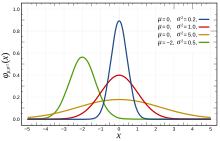
  кривая прижимается к оси абсцисс. Построим график нормальной плотности распределения при m = 0 и разных значениях параметра
  (Рис. 9):
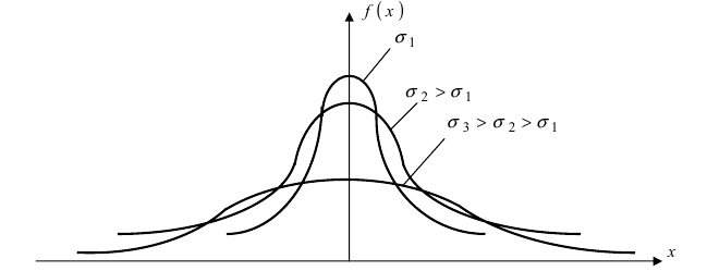
Рис. 9. Изменение графика плотности вероятности в зависимости от изменения средне-квадратичного отклонения при фиксированном значении математического ожидания.
Интегральная функция нормального распределения имеет вид: 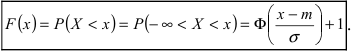
График функции распределения имеет вид (Рис. 10): 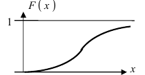
Рис. 10. Графика интегральной функции распределения нормальной случайной величины.
Вероятность попадания нормальной случайной величины в заданный интервал
Пусть требуется определить вероятность того, что нормальная случайная величина попадает в интервал  Согласно определению
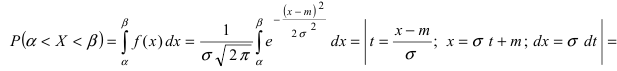 пересчитаем пределы интегрирования
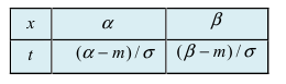
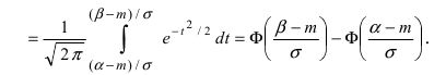 Следовательно,
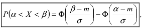
Рассмотрим основные свойства функции Лапласа Ф(х):
- Ф(0) = 0 — график функции Лапласа проходит через начало координат.
- Ф (-х) = — Ф(х) — функция Лапласа является нечетной функцией, поэтому
- таблицы для функции Лапласа приведены только для неотрицательных значений аргумента.
 — график функции Лапласа имеет горизонтальные асимптоты
 — график функции Лапласа имеет горизонтальные асимптоты
Следовательно, график функции Лапласа имеет вид (Рис. 11): 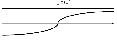
Рис. 11. График функции Лапласа.
Пример №1
Закон распределения нормальной случайной величины X имеет вид: 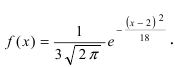 Определить вероятность попадания случайной величины X в интервал (-1;8).
Решение:
Согласно условиям задачи 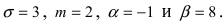 Поэтому искомая вероятность равна:
  0,4772 + 0,3413 = 0,8185.
Вычисление вероятности заданного отклонения
Вычисление вероятности заданного отклонения. Правило  .
.
Если интервал, в который попадает нормальная случайная величина X, симметричен относительно математического ожидания  то, используя свойство нечетности функции Лапласа, получим

Данная формула показывает, что отклонение случайной величины Х от ее математического ожидания на заданную величину l равна удвоенному значению функции Лапласа от отношения / к среднему квадратичному отклонению. Если положить  случаях нормальная случайная величина X отличается от своего математического ожидания на величину равную среднему квадратичному отклонению. Если
  то вероятность отклонения равна
  Наконец, в случае
  то вероятность отклонения равна
 Из последнего равенства видно, что только приблизительно в 0.3 % случаях отклонение нормальной случайной величины X от своего математического ожидания превышает
  Это свойство нормальной случайной величины X называется правилом “трех сигм”. На практике это правило применяется следующим образом: если отклонение случайной величины X от своего математического ожидания не превышает
  то эта случайная величина распределена по нормальному закону.
Показательный закон распределения
Определение: Закон распределения, определяемый фу нкцией распределения:
 называется экспоненциальным или показательным.
График экспоненциального закона распределения имеет вид (Рис. 12): 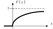
Рис. 12. График функции распределения для случая экспоненциального закона.
Дифференциальная функция распределения (плотность вероятности) имеет вид: 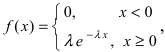 а ее график показан на (Рис. 13):
Рис. 13. График плотности вероятности для случая экспоненциального закона.
Пример №2
Случайная величина X подчиняется дифференциальной функции распределения  Найти вероятность того, что случайная величина X попадет в интервал (2; 4), математическое ожидание M[Х], дисперсию D[X] и среднее квадратичное отклонение
  Проверить выполнение правила “трех сигм” для показательного распределения.
Решение:
Интегральная функция распределения 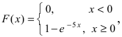 следовательно, вероятность того, что случайная величина X попадет в интервал (2; 4), равна:
  Математическое ожидание
 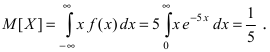 Вычислим значение величины М
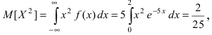 тогда дисперсия случайной величины X равна
 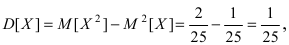 а средне-квадратичное
отклонение  Для проверки правила “трех сигм” вычислим вероятность заданного отклонения:
- Основные законы распределения вероятностей
- Асимптотика схемы независимых испытаний
- Функции случайных величин
- Центральная предельная теорема
- Повторные независимые испытания
- Простейший (пуассоновский) поток событий
- Случайные величины
- Числовые характеристики случайных величин
2.5.3. Нормальный закон распределения вероятностей
Без преувеличения его можно назвать философским законом. Наблюдая за различными объектами и процессами окружающего мира, мы часто
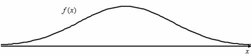
сталкиваемся с тем, что чего-то бывает мало, и что бывает норма. Перед вами принципиальный вид функции плотности нормального распределения вероятностей:
Какие можно примести примеры? Их просто тьма. Это, например, рост, вес людей (и не только), их физическая сила, умственные способности и
т.д. Существует «основная масса» (по тому или иному признаку) и существуют отклонения в обе стороны.
Это различные характеристики неодушевленных объектов (те же размеры, вес). Это случайная продолжительность процессов…, снова пришёл
на ум грустный пример, и поэтому скажу время «жизни» лампочек  Из физики вспомнились молекулы воздуха: среди них есть медленные, есть
быстрые, но большинство двигаются со «стандартными» скоростями.
Более того, даже дискретные распределения бывают близкИ к нормальному, и в конце
урока мы раскроем важную предпосылку «нормальности». А сейчас математика, математика, математика, которая в древности не зря считалась
философией!
Непрерывная случайная величина ![]() , распределённая по нормальному закону, имеет функцию
, распределённая по нормальному закону, имеет функцию
плотности  (не пугаемся) и однозначно
определяется параметрами ![]() и
и ![]() .
.
Эта функция получила фамилию некоронованного короля математики, К.Ф. Гаусса и в своё время была изображена вместе с его портретом
на купюре в 10 немецких марок. Для функции Гаусса выполнены общие свойства плотности, а
именно ![]() (почему?) и
(почему?) и  , откуда следует, что нормально
распределённая случайная величина достоверно примет одно из действительных значений. Теоретически – какое
угодно, практически – узнаем позже.
Следующие замечательные факты я тоже приведу без доказательства:
![]() – то есть, математическое ожидание нормально распределённой случайной величины в точности равно «а», а
– то есть, математическое ожидание нормально распределённой случайной величины в точности равно «а», а
среднее квадратическое отклонение в точности равно «сигме»: ![]() .
.
Эти значения выводятся с помощью общих формул, и желающие могут найти подробные выкладки в учебной литературе.
Ну а мы переходим к насущным практическим вопросам. Практики будет много, и она будет интересна не только «чайникам», но и более
подготовленным читателям:
Задача 118
Нормально распределённая случайная величина задана параметрами ![]() . Записать её функцию плотности и построить график.
. Записать её функцию плотности и построить график.
Несмотря на кажущуюся простоту задания, в нём существует немало тонкостей.
Первый момент касается обозначений. Они стандартные: матожидание обозначают буквой ![]() (реже
(реже ![]() или
или ![]() («мю»)), а стандартное отклонение – буквой
(«мю»)), а стандартное отклонение – буквой ![]() . Кстати, обратите внимание, что в условии ничего не
. Кстати, обратите внимание, что в условии ничего не
сказано о сущности параметров «а» и «сигма», и несведущий человек может только догадываться, что это такое.
Решение начнём шаблонной фразой: функция плотности нормально
распределённой случайной величины имеет вид  . В данном случае
 ![]() и:
и:

Первая, более лёгкая часть задачи выполнена. Теперь график. Вот на нём-то, на моей памяти, студентов «заворачивали» десятки раз,
причём, многих неоднократно. По той причине, что график функции Гаусса обладает несколькими принципиальными
особенностями, которые нужно обязательно отобразить на чертеже.
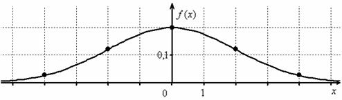
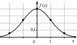
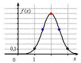
Сначала полная картина, затем комментарии:

На первом шаге декартову систему координат. При выполнении чертежа от руки во многих случаях оптимален следующий масштаб:
по оси абсцисс: 2 тетрадные клетки = 1 ед.,
по оси ординат: 2 тетрадные клетки = 0,1 ед., при этом саму ось следует расположить из тех соображений, что в точке ![]() функция достигает
функция достигает
максимума, и вертикальная прямая ![]() (на чертеже её нет) является линией симметрии
(на чертеже её нет) является линией симметрии
графика.
И логично, что в первую очередь удобно найти максимум функции:
Отмечаем вершину графика (красная точка).
Далее вычислим значения функции при ![]() , а точнее только одно из них – в силу симметрии графика они
, а точнее только одно из них – в силу симметрии графика они
равны:
Отмечаем синим цветом.
Внимание! ![]() и
и
![]() – это точки перегиба нормальной кривой. На интервале
– это точки перегиба нормальной кривой. На интервале
![]() график является
график является
выпуклым вверх, а на крайних интервалах – вогнутым вниз.
Далее отклоняемся от центра влево и право ещё на одно стандартное отклонение ![]() и рассчитываем высоту:
и рассчитываем высоту:
Отмечаем точки на чертеже (зелёный цвет) и видим, что этого вполне достаточно.
На завершающем этапе аккуратно чертим график, и особо аккуратно отражаем его выпуклость /
вогнутость! Ну и, наверное, вы давно поняли, что ось абсцисс – это горизонтальная асимптота, и «залезать» за неё
категорически нельзя!
Поговорим о том, как меняется форма нормальной кривой в зависимости от значений ![]() и
и ![]() .
.
При увеличении или уменьшении «а» (при неизменном «сигма») график сохраняет свою форму и перемещается вправо или
влево соответственно. Так, при ![]() (уменьшили «а» на 3) функция принимает вид
(уменьшили «а» на 3) функция принимает вид ![]() и наш график «переезжает»
и наш график «переезжает»
на 3 единицы влево – ровнехонько в начало координат:
Нормально распределённая величина с нулевым математическим ожиданием получила вполне естественное название – центрированная; её
функция плотности  –
–
чётная, и график симметричен относительно оси ординат.
В случае изменения «сигмы» (при постоянном «а»), график «остаётся на месте», но меняет форму. При увеличении ![]() он становится более
он становится более
низким и вытянутым, словно осьминог, растягивающий щупальца. И, наоборот, при уменьшении ![]() график становится более узким и высоким
график становится более узким и высоким
– как «удивлённый осьминог». Так, при уменьшении «сигмы» в два раза: ![]() предыдущий график сужается и вытягивается вверх в два
предыдущий график сужается и вытягивается вверх в два
раза:
Нормальное распределёние с единичным значением «сигма» называется нормированным, а если оно ещё и центрировано (наш
случай), то такое распределение называют стандартным. Оно имеет ещё более простую функцию плотности, которая уже встречалась в локальной теореме Лапласа: ![]() . Стандартное распределение нашло широкое применение, и
. Стандартное распределение нашло широкое применение, и
очень скоро мы окончательно поймём его предназначение.
И как-то незаслуженно осталась в тени функция распределения вероятностей.
Вспоминаем её определение:
 –
–
вероятность того, что случайная величина ![]() примет значение, МЕНЬШЕЕ, чем переменная
примет значение, МЕНЬШЕЕ, чем переменная ![]() , которая «пробегает» все
, которая «пробегает» все
действительные значения до «плюс» бесконечности.
Внутри интеграла используют другую букву, чтобы не возникало «накладок» с обозначениями, ибо здесь каждому значению ![]() ставится в соответствие
ставится в соответствие
несобственный интеграл  , который равен некоторому числу из интервала
![]() . Почти все значения
. Почти все значения
![]() не поддаются
не поддаются
абсолютно точному расчету, но с современными вычислительными мощностями с этим нет никаких трудностей (ролик на Ютубе).
Так, например, график функции  стандартного распределения
 ![]() имеет следующий вид:
имеет следующий вид:

На чертеже хорошо видно выполнение всех свойств функции распределения, и из
технических нюансов здесь следует обратить внимание на горизонтальные асимптоты и точку перегиба ![]() .
.
Теперь вспомним одну из ключевых задач темы, а именно выясним, как найти ![]() – вероятность того, что
– вероятность того, что
нормальная случайная величина ![]() примет
примет
значение из интервала ![]() . Геометрически эта вероятность равна площади между
. Геометрически эта вероятность равна площади между
нормальной кривой и осью абсцисс на соответствующем участке:
но каждый раз вымучивать приближенное значение  неразумно, и поэтому здесь рациональнее использовать
«лёгкую» формулу:
![]()
! Вспоминает также, что:
![]()
Тут можно снова задействовать Эксель, но есть пара весомых «но»: во-первых, он не всегда под рукой, а во-вторых, «готовые» значения
![]() , скорее всего,
, скорее всего,
вызовут вопросы у преподавателя. Почему?
Об этом я неоднократно рассказывал ранее: в своё время (и ещё не очень давно) роскошью был обычный калькулятор, и в учебной
литературе до сих пор сохранился «ручной» способ решения рассматриваемой задачи. Его суть состоит в том, чтобы свести решение к
стандартному распределению:
![]() , где
, где

Зачем это нужно? Дело в том, что значения ![]() скрупулезно подсчитаны нашими предками и сведены в
скрупулезно подсчитаны нашими предками и сведены в
специальную таблицу, которая есть во многих книгах по терверу. Но ещё чаще встречается таблица значений функции Лапласа:
 , и с этой
функцией и этой таблицей (см. Приложение Таблицы) мы уже имели дело в интегральной теореме Лапласа.
Итак, вероятность того, что нормальная случайная величина ![]() с параметрами
с параметрами ![]() и
и ![]() примет значение из интервала
примет значение из интервала ![]() , можно вычислить по формуле:
, можно вычислить по формуле:
![]() , где
, где ![]() – функция Лапласа.
– функция Лапласа.
Таким образом, наша задача становится чуть ли не устной! Порой, здесь хмыкают и говорят, что метод устарел. Может быть…, но
парадокс состоит в том, что «устаревший метод» очень быстро приводит к результату!
И ещё в этом заключена большая мудрость – если вдруг пропадёт электричество или восстанут машины, то у человечества останется
возможность заглянуть в бумажные таблицы и спасти мир =) Классика жанра:
Задача 119
Из пункта ![]() ведётся стрельба из орудия вдоль прямой
ведётся стрельба из орудия вдоль прямой ![]() . Предполагается, что дальность
. Предполагается, что дальность
полёта распределена нормально с математическим ожиданием 1000 м и средним квадратическим отклонением 5 м. Определить (в процентах) сколько
снарядов упадёт с перелётом от 5 до 70м.
Решение: в задаче рассматривается нормально распределённая случайная величина ![]() – дальность полёта снаряда, и по
– дальность полёта снаряда, и по
условию ![]() .
.
Так как речь идёт о перелёте за цель, то ![]() . Вычислим вероятность
. Вычислим вероятность ![]() – того, что снаряд упадёт в пределах этой
– того, что снаряд упадёт в пределах этой
дистанции.
Если в вашей методичке дана таблица значений функции  , то используйте формулу
 ![]() :
:

Для самопроверки можно «забить» ![]() и затем
и затем ![]() в Пункт 9
в Пункт 9
Калькулятора, и кроме того, для стандартного нормального распределения в Экселе существует прямая функция
=НОРМСТРАСП(z).
Но гораздо чаще, и в этом курсе в частности, встречается таблица значений функции Лапласа  , поэтому решаем через неё:

Дробные значения традиционно округляем до 4 знаков после запятой, как это сделано в типовой таблице. И для контроля есть Пункт
5 макета.
Напоминаю, что ![]() . Всегда контролируйте, таблица КАКОЙ функции
. Всегда контролируйте, таблица КАКОЙ функции
перед вашими глазами.
Ответ требуется дать в процентах, поэтому рассчитанную вероятность нужно умножить на 100 и снабдить результат
содержательным комментарием:
– с перелётом от 5 до 70 м упадёт примерно 15,87% снарядов
Тренируемся самостоятельно:
Задача 120
Диаметр подшипников, изготовленные на заводе, представляет собой случайную величину, распределенную нормально с математическим
ожиданием 1,5 см и средним квадратическим отклонением 0,04 см. Найти вероятность того, что размер наугад взятого подшипника колеблется от
1,4 до 1,6 см.
В образце решения и далее я буду использовать функцию Лапласа, как самый распространённый вариант. Кстати, обратите внимание, что
согласно формулировке, в этой задаче корректнее будет включить концы интервала в рассмотрение.
И уже в этом примере нам встретился особый случай – когда интервал ![]() симметричен относительно математического ожидания. В
симметричен относительно математического ожидания. В
такой ситуации его можно записать в виде ![]() и, пользуясь нечётностью функции Лапласа
и, пользуясь нечётностью функции Лапласа ![]() , упростить рабочую
, упростить рабочую
формулу ![]() :
:

Параметр «дельта» называют отклонением от математического ожидания, и двойное неравенство удобно «упаковать» с помощью модуля:
![]() –
–
вероятность того, что значение случайной величины ![]() отклонится от математического ожидания менее чем на
отклонится от математического ожидания менее чем на
![]() .
.
Таким, образом задача про подшипники решается гораздо короче:
![]() –
–
вероятность того, что диаметр наугад взятого подшипника отличается от 1,5 см не более чем на 0,1 см.
Результат этой задачи получился близким к единице, но хотелось бы ещё бОльшей надежности – а именно, узнать границы, в которых
находится диаметр почти всех подшипников. Существует ли какой-нибудь критерий на этот счёт? Существует! На этот вопрос отвечает
так называемое правило «трех сигм».
Его суть состоит в том, что практически достоверным является тот факт, что
нормально распределённая случайная величина ![]() примет значение из промежутка
примет значение из промежутка ![]() . И в самом деле, вероятность
. И в самом деле, вероятность
отклонения от матожидания менее чем на ![]() составляет:
составляет:
![]() или
или
99,73%
В «пересчёте на подшипники» – это 9973 штуки с диаметром от 1,38 до 1,62 см и всего лишь 27 «некондиционных» экземпляров.
Продолжаем решать суровые советские задачи:
Задача 121
Случайная величина ![]() ошибки взвешивания распределена по нормальному закону
ошибки взвешивания распределена по нормальному закону
с нулевым математическим ожиданием и стандартным отклонением 3 грамма. Найти вероятность того, что очередное взвешивание будет проведено с
ошибкой, не превышающей по модулю 5 грамм.
Решение очень простое. По условию, ![]() и сразу заметим, что по правилу «трёх сигм», при
и сразу заметим, что по правилу «трёх сигм», при
очередном взвешивании (чего-то или кого-то) мы почти 100% получим погрешность менее 9 грамм. Но в задаче фигурирует более узкое
отклонение ![]() и по
и по
формуле ![]() :
:
![]() –
–
вероятность того, что очередное взвешивание будет проведено с ошибкой, не превышающей 5 грамм.
Ответ: ![]()
Этот пример принципиально отличается от вроде бы похожей задачи параграфа о равномерном распределении. Там была погрешность округления результатов измерений,
здесь же речь идёт о случайной погрешности самих измерений. Такие погрешности возникают в связи с техническими характеристиками самого
прибора (диапазон допустимых ошибок, как правило, указывают в его паспорте), а также по вине самого экспериментатора – когда мы,
например, «на глазок» снимаем показания со стрелки механических весов.
Помимо прочих, существуют ещё так называемые систематические ошибки измерения. Это уже неслучайные ошибки, которые
возникают по причине некорректной настройки или эксплуатации прибора. Так, например, неотрегулированные напольные весы могут стабильно
«прибавлять» килограмм, а продавец систематически обвешивать покупателей. Или не систематически, ведь можно обсчитать Однако, в любом
случае, случайной такая «ошибка» не будет, и её матожидание отлично от нуля.
…срочно разрабатываю курс по подготовке продавцов =)
Самостоятельно решаем обратную задачу:
Задача 122
Диаметр валика – случайная нормально распределенная случайная величина, среднее квадратическое отклонение ее равно ![]() мм. Найти длину интервала,
мм. Найти длину интервала,
симметричного относительно математического ожидания, в который с вероятностью ![]() попадет длина диаметра валика.
попадет длина диаметра валика.
Пункт 5* Калькулятора в помощь. Обратите внимание, что здесь не известно математическое ожидание,
но это нисколько не мешает решить поставленную задачу.
И экзаменационное задание, которое я настоятельно рекомендую для закрепления материала:
Задача 123
Нормально распределенная случайная величина ![]() задана своими параметрами
задана своими параметрами ![]() (математическое ожидание) и
(математическое ожидание) и ![]() (среднее квадратическим отклонение).
(среднее квадратическим отклонение).
Требуется:
а) записать плотность вероятности и схематически изобразить ее график;
б) найти вероятность того, что ![]() примет значение из интервала
примет значение из интервала ![]() ;
;
в) найти вероятность того, что ![]() отклонится по модулю от
отклонится по модулю от ![]() не более чем на
не более чем на ![]() ;
;
г) применяя правило «трех сигм», найти значения случайной величины ![]() .
.
Такие задачи предлагаются повсеместно, и за годы практики мне их довелось решить сотни и сотни штук. Обязательно попрактикуйтесь в
ручном построении чертежа и использовании таблицы  После чего мы разберём заключительный пример:
Задача 124
Плотность распределения вероятностей случайной величины ![]() имеет вид
имеет вид ![]() . Найти
. Найти ![]() , математическое ожидание
, математическое ожидание ![]() , дисперсию
, дисперсию ![]() , функцию распределения
, функцию распределения ![]() , построить графики плотности и
, построить графики плотности и
функции распределения, найти ![]() .
.
Решение: прежде всего, обратим внимание, что в условии ничего не сказано о характере случайной величины. Само по
себе присутствие экспоненты ещё ничего не значит: это может оказаться, например, показательное или вообще произвольное непрерывное распределение. И поэтому «нормальность» распределения ещё нужно обосновать:
функция ![]() определена при любом действительном значении
определена при любом действительном значении
![]() , и если её
, и если её
удастся привести к виду  , то случайная величина
 ![]() распределена по нормальному закону.
распределена по нормальному закону.
Пробуем привести. Для этого выделяем полный квадрат и
организуем трёхэтажную дробь:

Обязательно выполняем проверку, возвращая показатель в исходный вид:

![]() , что мы и
, что мы и
хотели увидеть.
Таким образом, мы действительно имеем дело с нормальным распределением:
 – по
– по
правилу действий со степенями «отщипываем» ![]() . И здесь можно сразу записать очевидные числовые
. И здесь можно сразу записать очевидные числовые
характеристики:
![]()
Теперь найдём значение параметра ![]() . Поскольку множитель нормального распределения имеет
. Поскольку множитель нормального распределения имеет
вид ![]() и
и ![]() , то:
, то:
 , откуда
выражаем ![]() и
и
подставляем в нашу функцию:
 , после чего
ещё раз пробежим глазами и убедимся, что полученная функция имеет вид  .
.
Построим график плотности:
и график функции распределения  :
:
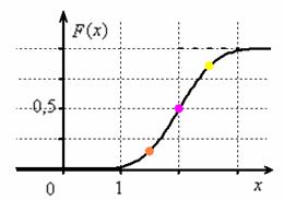
Пару слов на счёт ручного построения последнего графика – на случай отсутствия под рукой Экселя или даже обычного калькулятора. В
точке ![]() функция
функция
распределения принимает значение ![]() и здесь находится перегиб графика (малиновая точка).
и здесь находится перегиб графика (малиновая точка).
Кроме того, для более или менее приличного чертежа желательно найти ещё хотя бы пару точек. Берём традиционное значение ![]() и
и
стандартизируем его по формуле ![]() . Далее по таблице значений функции Лапласа находим:
. Далее по таблице значений функции Лапласа находим: ![]() – жёлтая точка на
– жёлтая точка на
чертеже. С симметричной оранжевой точкой никаких проблем: ![]() и:
и:
![]() .
.
После чего аккуратно проводим интегральную кривую, не забывая о перегибе и двух горизонтальных асимптотах.
Да, и ещё нужно вычислить:
![]()
![]() –
–
вероятность того, что случайная величина ![]() примет значение из данного отрезка.
примет значение из данного отрезка.
Задача была непростой, и посему блеснём академичным стилем, ответ: 
А теперь обещанный секрет:
понятие о центральной предельной теореме.
которую также называют теоремой Ляпунова. Её суть состоит в том, что если случайная величина ![]() является суммой очень большого числа взаимно
является суммой очень большого числа взаимно
независимых случайных величин ![]() , влияние каждой из которых на всю сумму ничтожно мало, то
, влияние каждой из которых на всю сумму ничтожно мало, то
![]() имеет
имеет
распределение, близкое к нормальному.
В окружающем мире условие теоремы Ляпунова выполняется очень часто, и поэтому нормальное распределение встречается буквально на
каждом шагу.
Так, например, молекул воздуха очень и очень много, и каждая из них своим движением оказывает ничтожно малое влияние на всю
совокупность. Поэтому скорость молекул воздуха распределена нормально.
Большая популяция некоторых особей. Каждая из них (или подавляющее большинство) оказывает несущественное влияние на жизнь всей
популяции, следовательно, продолжительность жизни этих особей тоже распределена по нормальному закону.
Теперь вернёмся к знакомой задаче, где проводится ![]() независимых
независимых
испытаний, в каждом из которых некое событие ![]() может появиться с постоянной вероятностью
может появиться с постоянной вероятностью ![]() . Эти испытания можно
. Эти испытания можно
считать попарно независимым случайными величинами ![]() , и при достаточно большом значении «эн» биномиальное распределение случайной величины
, и при достаточно большом значении «эн» биномиальное распределение случайной величины ![]() – числа появлений события
– числа появлений события ![]() в
в ![]() испытаниях – очень близко к
испытаниях – очень близко к
нормальному распределению.
Уже при ![]() и
и ![]() в многоугольнике биномиального распределения хорошо просматривается нормальная кривая:
в многоугольнике биномиального распределения хорошо просматривается нормальная кривая:
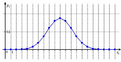
И чем больше ![]() , тем ближе будет сходство. Причём, вероятность
, тем ближе будет сходство. Причём, вероятность ![]() может быть любой, но
может быть любой, но
не слишком малой.
Именно этот факт мы и использовали в теоремах Лапласа – когда приближали биномиальные
вероятности соответствующими значениями функций нормального распределения.
Подчёркиваю, что теорема Ляпунова носит статус теоремы, а значит, строго доказана в теории.
И в заключение книги хочется ответить на один философский вопрос: имеет ли в нашей жизни значение случайность? Безусловно! Везение
играет немаловажную, а порой, и огромную роль: встретить хороших друзей, встретить «своего» человека, найти деятельность по душе и т.д. –
всё это нередко происходит благодаря случаю….
Но, с другой стороны, гораздо более важнА системная и упорная деятельность, после которой следуют закономерные результаты.
Желательно, полезные, конечно J
Дополнительную информацию можно найти в соответствующем разделе портала mathprofi.ru (ссылка
на карту раздела). Из учебной литературы рекомендую:
Гмурман В. Е. Теория вероятностей и математическая статистика (уч. пособие);
Гмурман В. Е. Руководство к решению задач по теории вероятности (задачник с примерами решений).
Везения в главном!
 2.5.2. Показательное распределение вероятностей
| Оглавление |
Полную и свежую версию этой книги в pdf-формате,
а также курсы по другим темам можно найти здесь.
Также вы можете изучить эту тему подробнее – просто, доступно, весело и бесплатно!
С наилучшими пожеланиями, Александр Емелин
Нормальным называют распределение вероятностей непрерывной случайной величины
, плотность которого имеет вид:
где
–
математическое ожидание,
–
среднее квадратическое отклонение
.
Вероятность того, что
примет
значение, принадлежащее интервалу
:
где
– функция Лапласа:
Вероятность того, что абсолютная
величина отклонения меньше положительного числа
:
В частности, при
справедливо
равенство:
Асимметрия, эксцесс,
мода и медиана нормального распределения соответственно равны:
, где
Правило трех сигм
Преобразуем формулу:
Положив
. В итоге получим
если
, и, следовательно,
, то
то есть вероятность того, что
отклонение по абсолютной величине будет меньше утроенного среднего квадратического отклонение, равна 0,9973.
Другими словами, вероятность того,
что абсолютная величина отклонения превысит утроенное среднее квадратическое отклонение, очень мала, а именно равна
0,0027. Это означает, что лишь в 0,27% случаев так может произойти. Такие
события исходя из принципа невозможности маловероятных
событий можно считать практически невозможными. В этом и состоит
сущность правила трех сигм: если случайная величина распределена нормально, то
абсолютная величина ее отклонения от математического ожидания не превосходит
утроенного среднего квадратического отклонения.
На практике правило трех сигм
применяют так: если распределение изучаемой случайной величины неизвестно, но
условие, указанное в приведенном правиле, выполняется, то есть основание
предполагать, что изучаемая величина распределена нормально; в противном случае
она не распределена нормально.
Смежные темы решебника:
- Таблица значений функции Лапласа
- Непрерывная случайная величина
- Показательный закон распределения случайной величины
- Равномерный закон распределения случайной величины
Пример 2
Ошибка
высотометра распределена нормально с математическим ожиданием 20 мм и средним
квадратичным отклонением 10 мм.
а) Найти
вероятность того, что отклонение ошибки от среднего ее значения не превзойдет 5
мм по абсолютной величине.
б) Какова
вероятность, что из 4 измерений два попадут в указанный интервал, а 2 – не
превысят 15 мм?
в)
Сформулируйте правило трех сигм для данной случайной величины и изобразите
схематично функции плотности вероятностей и распределения.
Решение
На сайте можно заказать решение контрольной или самостоятельной работы, домашнего задания, отдельных задач. Для этого вам нужно только связаться со мной:
ВКонтакте
WhatsApp
Telegram
Мгновенная связь в любое время и на любом этапе заказа. Общение без посредников. Удобная и быстрая оплата переводом на карту СберБанка. Опыт работы более 25 лет.
Подробное решение в электронном виде (docx, pdf) получите точно в срок или раньше.
а) Вероятность того, что случайная величина, распределенная по
нормальному закону, отклонится от среднего не более чем на величину
:
В нашем
случае получаем:
б) Найдем
вероятность того, что отклонение ошибки от среднего значения не превзойдет 15
мм:
Пусть событие
– ошибки 2
измерений не превзойдут 5 мм и ошибки 2 измерений не превзойдут 0,8664 мм
– ошибка не
превзошла 5 мм;
– ошибка не
превзошла 15 мм
в)
Для заданной нормальной величины получаем следующее правило трех сигм:
Ошибка высотометра будет лежать в интервале:
Функция плотности вероятностей:
График плотности распределения нормально распределенной случайной величины
Функция распределения:
График функции
распределения нормально распределенной случайной величины
Задача 1
Среднее
количество осадков за июнь 19 см. Среднеквадратическое отклонение количества
осадков 5 см. Предполагая, что количество осадков нормально-распределенная
случайная величина найти вероятность того, что будет не менее 13 см осадков.
Какой уровень превзойдет количество осадков с вероятностью 0,95?
Задача 2
Найти
закон распределения среднего арифметического девяти измерений нормальной
случайной величины с параметрами m=1.0 σ=3.0. Чему равна вероятность того, что
модуль разности между средним арифметическим и математическим ожиданием
превысит 0,5?
Указание:
воспользоваться таблицами нормального распределения (функции Лапласа).
Задача 3
Отклонение
напряжения в сети переменного тока описывается нормальным законом
распределения. Дисперсия составляет 20 В. Какова вероятность при изменении
выйти за пределы требуемых 10% (22 В).
На сайте можно заказать решение контрольной или самостоятельной работы, домашнего задания, отдельных задач. Для этого вам нужно только связаться со мной:
ВКонтакте
WhatsApp
Telegram
Мгновенная связь в любое время и на любом этапе заказа. Общение без посредников. Удобная и быстрая оплата переводом на карту СберБанка. Опыт работы более 25 лет.
Подробное решение в электронном виде (docx, pdf) получите точно в срок или раньше.
Задача 4
Автомат
штампует детали. Контролируется длина детали Х, которая распределена нормально
с математическим ожиданием (проектная длинна), равная 50 мм. Фактическая длина
изготовленных деталей не менее 32 и не более 68 мм. Найти вероятность того, что
длина наудачу взятой детали: а) больше 55 мм; б) меньше 40 мм.
Задача 5
Случайная
величина X распределена нормально с математическим ожиданием a=10и средним
квадратическим отклонением σ=5. Найти
интервал, симметричный относительно математического ожидания, в котором с
вероятностью 0,9973 попадает величина Х в результате испытания.
Задача 6
Заданы
математическое ожидание ax=19 и среднее квадратическое отклонение σ=4
нормально распределенной случайной величины X. Найти: 1) вероятность
того, что X примет значение, принадлежащее интервалу (α=15;
β=19); 2) вероятность того, что абсолютная величина отклонения значения
величины от математического ожидания окажется меньше δ=18.
Задача 7
Диаметр
выпускаемой детали – случайная величина, распределенная по нормальному закону с
математическим ожиданием и дисперсией, равными соответственно 10 см и 0,16 см2.
Найти вероятность того, что две взятые наудачу детали имеют отклонение от
математического ожидания по абсолютной величине не более 0,16 см.
Задача 8
Ошибка
прогноза температуры воздуха есть случайная величина с m=0,σ=2℃. Найти вероятность
того, что в течение недели ошибка прогноза трижды превысит по абсолютной
величине 4℃.
Задача 9
Непрерывная
случайная величина X распределена по нормальному
закону: X∈N(a,σ).
а) Написать
плотность распределения вероятностей и функцию распределения.
б) Найти
вероятность того, что в результате испытания случайная величина примет значение
из интервала (α,β).
в) Определить
приближенно минимальное и максимальное значения случайной величины X.
г) Найти
интервал, симметричный относительно математического ожидания a, в котором с
вероятностью 0,98 будут заключены значения X.
a=5; σ=1.3;
α=4; β=6
Задача 10
Производится измерение вала без
систематических ошибок. Случайные ошибки измерения X
подчинены нормальному закону с σx=10. Найти вероятность того, что измерение будет
произведено с ошибкой, превышающей по абсолютной величине 15 мм.
Задача 11
Высота
стебля озимой пшеницы — случайная величина, распределенная по нормальному закону
с параметрами a = 75 см, σ = 1 см. Найти вероятность того, что высота стебля:
а) окажется от 72 до 80 см; б) отклонится от среднего не более чем на 0,5 см.
Задача 12
Деталь,
изготовленная автоматом, считается годной, если отклонение контролируемого
размера от номинала не превышает 10 мм. Точность изготовления деталей
характеризуется средним квадратическим отклонением, при данной технологии
равным 5 мм.
а)
Считая, что отклонение размера детали от номинала есть нормально распределенная
случайная величина, найти долю годных деталей, изготовляемых автоматом.
б) Какой
должна быть точность изготовления, чтобы процент годных деталей повысился до
98?
в)
Написать выражение для функции плотности вероятности и распределения случайной
величины.
Задача 13
Диаметр
детали, изготовленной цехом, является случайной величиной, распределенной по
нормальному закону. Дисперсия ее равна 0,0001 см, а математическое ожидание –
2,5 см. Найдите границы, симметричные относительно математического ожидания, в
которых с вероятностью 0,9973 заключен диаметр наудачу взятой детали. Какова
вероятность того, что в серии из 1000 испытаний размер диаметра двух деталей
выйдет за найденные границы?
На сайте можно заказать решение контрольной или самостоятельной работы, домашнего задания, отдельных задач. Для этого вам нужно только связаться со мной:
ВКонтакте
WhatsApp
Telegram
Мгновенная связь в любое время и на любом этапе заказа. Общение без посредников. Удобная и быстрая оплата переводом на карту СберБанка. Опыт работы более 25 лет.
Подробное решение в электронном виде (docx, pdf) получите точно в срок или раньше.
Задача 14
Предприятие
производит детали, размер которых распределен по нормальному закону с
математическим ожиданием 20 см и стандартным отклонением 2 см. Деталь будет
забракована, если ее размер отклонится от среднего (математического ожидания)
более, чем на 2 стандартных отклонения. Наугад выбрали две детали. Какова вероятность
того, что хотя бы одна из них будет забракована?
Задача 15
Диаметры
деталей распределены по нормальному закону. Среднее значение диаметра равно d=14 мм
, среднее квадратическое
отклонение σ=2 мм
. Найти вероятность того,
что диаметр наудачу взятой детали будет больше α=15 мм и не меньше β=19 мм; вероятность того, что диаметр детали
отклонится от стандартной длины не более, чем на Δ=1,5 мм.
Задача 16
В
электропечи установлена термопара, показывающая температуру с некоторой
ошибкой, распределенной по нормальному закону с нулевым математическим
ожиданием и средним квадратическим отклонением σ=10℃. В момент когда термопара
покажет температуру не ниже 600℃, печь автоматически отключается. Найти
вероятность того, что печь отключается при температуре не превышающей 540℃ (то
есть ошибка будет не меньше 30℃).
Задача 17
Длина
детали представляет собой нормальную случайную величину с математическим
ожиданием 40 мм и среднеквадратическим отклонением 3 мм. Найти:
а)
Вероятность того, что длина взятой наугад детали будет больше 34 мм и меньше 43
мм;
б)
Вероятность того, что длина взятой наугад детали отклонится от ее
математического ожидания не более, чем на 1,5 мм.
Задача 18
Случайное
отклонение размера детали от номинала распределены нормально. Математическое
ожидание размера детали равно 200 мм, среднее квадратическое отклонение равно
0,25 мм, стандартами считаются детали, размер которых заключен между 199,5 мм и
200,5 мм. Из-за нарушения технологии точность изготовления деталей уменьшилась
и характеризуется средним квадратическим отклонением 0,4 мм. На сколько
повысился процент бракованных деталей?
Задача 19
Случайная
величина X~N(1,22). Найти P{2
На сайте можно заказать решение контрольной или самостоятельной работы, домашнего задания, отдельных задач. Для этого вам нужно только связаться со мной:
ВКонтакте
WhatsApp
Telegram
Мгновенная связь в любое время и на любом этапе заказа. Общение без посредников. Удобная и быстрая оплата переводом на карту СберБанка. Опыт работы более 25 лет.
Подробное решение в электронном виде (docx, pdf) получите точно в срок или раньше.
Задача 20
Заряд пороха для охотничьего ружья
должен составлять 2,3 г. Заряд отвешивается на весах, имеющих ошибку
взвешивания, распределенную по нормальному закону со средним квадратическим
отклонением, равным 0,2 г. Определить вероятность повреждения ружья, если максимально
допустимый вес заряда составляет 2,8 г.
Задача 21
Заряд
охотничьего пороха отвешивается на весах, имеющих среднеквадратическую ошибку
взвешивания 150 мг. Номинальный вес порохового заряда 2,3 г. Определить
вероятность повреждения ружья, если максимально допустимый вес порохового
заряда 2,5 г.
Задача 21
Найти
вероятность попадания снарядов в интервал (α1=10.7; α2=11.2).
Если случайная величина X распределена по
нормальному закону с параметрами m=11;
σ=0.2.
Задача 22
Плотность
вероятности распределения случайной величины имеет вид
Найти
вероятность того, что из 3 независимых случайных величин, распределенных по
данному закону, 3 окажутся на интервале (-∞;5).
Задача 23
Непрерывная
случайная величина имеет нормальное распределение. Её математическое ожидание
равно 12, среднее квадратичное отклонение равно 2. Найти вероятность того, что
в результате испытания случайная величина примет значение в интервале (8,14)
Задача 24
Вероятность
попадания нормально распределенной случайной величины с математическим
ожиданием m=4 в интервал (3;5) равна 0,6. Найти дисперсию данной случайной
величины.
Задача 25
В
нормально распределенной совокупности 17% значений случайной величины X
меньше 13% и 47% значений случайной величины X
больше 19%. Найти параметры этой совокупности.
Задача 26
Студенты
мужского пола образовательного учреждения были обследованы на предмет
физических характеристик и обнаружили, что средний рост составляет 182 см, со
стандартным отклонением 6 см. Предполагая нормальное распределение для роста,
найдите вероятность того, что конкретный студент-мужчина имеет рост более 185
см.
|
Probability density function
The red curve is the standard normal distribution |
|
|
Cumulative distribution function
|
|
| Notation |
 |
|---|---|
| Parameters |
 = mean (location) = mean (location) = variance (squared scale) = variance (squared scale) |
| Support |
 |
 |
|
| CDF |
![{displaystyle {frac {1}{2}}left[1+operatorname {erf} left({frac {x-mu }{sigma {sqrt {2}}}}right)right]}](https://wikimedia.org/api/rest_v1/media/math/render/svg/187f33664b79492eedf4406c66d67f9fe5f524ea) |
| Quantile |
 |
| Mean |
 |
| Median |
|
| Mode |
|
| Variance |
 |
| MAD |
 |
| Skewness |
 |
| Ex. kurtosis |
|
| Entropy |
 |
| MGF |
 |
| CF |
 |
| Fisher information |
|
| Kullback-Leibler divergence |
 |
| CVaR (ES) |
 [1] [1] |


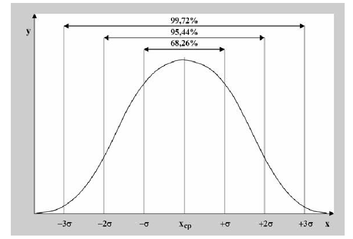
In statistics, a normal distribution or Gaussian distribution is a type of continuous probability distribution for a real-valued random variable. The general form of its probability density function is

The parameter is the mean or expectation of the distribution (and also its median and mode), while the parameter  is its standard deviation. The variance of the distribution is . A random variable with a Gaussian distribution is said to be normally distributed, and is called a normal deviate.
Normal distributions are important in statistics and are often used in the natural and social sciences to represent real-valued random variables whose distributions are not known.[2][3] Their importance is partly due to the central limit theorem. It states that, under some conditions, the average of many samples (observations) of a random variable with finite mean and variance is itself a random variable—whose distribution converges to a normal distribution as the number of samples increases. Therefore, physical quantities that are expected to be the sum of many independent processes, such as measurement errors, often have distributions that are nearly normal.[4]
Moreover, Gaussian distributions have some unique properties that are valuable in analytic studies. For instance, any linear combination of a fixed collection of normal deviates is a normal deviate. Many results and methods, such as propagation of uncertainty and least squares parameter fitting, can be derived analytically in explicit form when the relevant variables are normally distributed.
A normal distribution is sometimes informally called a bell curve.[5] However, many other distributions are bell-shaped (such as the Cauchy, Student’s t, and logistic distributions). For other names, see Naming.
The univariate probability distribution is generalized for vectors in the multivariate normal distribution and for matrices in the matrix normal distribution.
Definitions[edit]
Standard normal distribution[edit]
The simplest case of a normal distribution is known as the standard normal distribution or unit normal distribution. This is a special case when  and
and  , and it is described by this probability density function (or density):

The variable  has a mean of 0 and a variance and standard deviation of 1. The density
  has its peak
  at
at  and inflection points at
  and
and  .
.
Although the density above is most commonly known as the standard normal, a few authors have used that term to describe other versions of the normal distribution. Carl Friedrich Gauss, for example, once defined the standard normal as

which has a variance of 1/2, and Stephen Stigler[6] once defined the standard normal as

which has a simple functional form and a variance of 
General normal distribution[edit]
Every normal distribution is a version of the standard normal distribution, whose domain has been stretched by a factor (the standard deviation) and then translated by (the mean value):

The probability density must be scaled by  so that the integral is still 1.
If  is a standard normal deviate, then
  will have a normal distribution with expected value and standard deviation . This is equivalent to saying that the «standard» normal distribution can be scaled/stretched by a factor of and shifted by to yield a different normal distribution, called
  . Conversely, if is a normal deviate with parameters and , then this distribution can be re-scaled and shifted via the formula
  to convert it to the «standard» normal distribution. This variate is also called the standardized form of .
Notation[edit]
The probability density of the standard Gaussian distribution (standard normal distribution, with zero mean and unit variance) is often denoted with the Greek letter  (phi).[7] The alternative form of the Greek letter phi,
  , is also used quite often.
The normal distribution is often referred to as  or .[8] Thus when a random variable is normally distributed with mean and standard deviation , one may write

Alternative parameterizations[edit]
Some authors advocate using the precision  as the parameter defining the width of the distribution, instead of the deviation or the variance . The precision is normally defined as the reciprocal of the variance,
  .[9] The formula for the distribution then becomes

This choice is claimed to have advantages in numerical computations when is very close to zero, and simplifies formulas in some contexts, such as in the Bayesian inference of variables with multivariate normal distribution.
Alternatively, the reciprocal of the standard deviation  might be defined as the precision, in which case the expression of the normal distribution becomes

According to Stigler, this formulation is advantageous because of a much simpler and easier-to-remember formula, and simple approximate formulas for the quantiles of the distribution.
Normal distributions form an exponential family with natural parameters  and
and  , and natural statistics x and x2. The dual expectation parameters for normal distribution are η1 = μ and η2 = μ2 + σ2.
Cumulative distribution functions[edit]
The cumulative distribution function (CDF) of the standard normal distribution, usually denoted with the capital Greek letter  (phi), is the integral

The related error function  gives the probability of a random variable, with normal distribution of mean 0 and variance 1/2 falling in the range
 ![[-x,x]](https://wikimedia.org/api/rest_v1/media/math/render/svg/e23c41ff0bd6f01a0e27054c2b85819fcd08b762) . That is:
. That is:

These integrals cannot be expressed in terms of elementary functions, and are often said to be special functions. However, many numerical approximations are known; see below for more.
The two functions are closely related, namely
![{displaystyle Phi (x)={frac {1}{2}}left[1+operatorname {erf} left({frac {x}{sqrt {2}}}right)right]}](https://wikimedia.org/api/rest_v1/media/math/render/svg/c7831a9a5f630df7170fa805c186f4c53219ca36)
For a generic normal distribution with density  , mean and deviation , the cumulative distribution function is
![{displaystyle F(x)=Phi left({frac {x-mu }{sigma }}right)={frac {1}{2}}left[1+operatorname {erf} left({frac {x-mu }{sigma {sqrt {2}}}}right)right]}](https://wikimedia.org/api/rest_v1/media/math/render/svg/75deccfbc473d782dacb783f1524abb09b8135c0)
The complement of the standard normal CDF,  , is often called the Q-function, especially in engineering texts.[10][11] It gives the probability that the value of a standard normal random variable will exceed
  :
:  . Other definitions of the
  -function, all of which are simple transformations of , are also used occasionally.[12]
The graph of the standard normal CDF has 2-fold rotational symmetry around the point (0,1/2); that is,  . Its antiderivative (indefinite integral) can be expressed as follows:

The CDF of the standard normal distribution can be expanded by Integration by parts into a series:
![{displaystyle Phi (x)={frac {1}{2}}+{frac {1}{sqrt {2pi }}}cdot e^{-x^{2}/2}left[x+{frac {x^{3}}{3}}+{frac {x^{5}}{3cdot 5}}+cdots +{frac {x^{2n+1}}{(2n+1)!!}}+cdots right]}](https://wikimedia.org/api/rest_v1/media/math/render/svg/54d12af9a3b12a7f859e4e7be105d172b53bcfb8)
where  denotes the double factorial.
An asymptotic expansion of the CDF for large x can also be derived using integration by parts. For more, see Error function#Asymptotic expansion.[13]
A quick approximation to the standard normal distribution’s CDF can be found by using a Taylor series approximation:

Recursive computation with Taylor Series expansion[edit]
The recursive nature of the  family of derivatives may be used to easily construct a rapidly converging Taylor series expansion using recursive entries about any point of known value of the distribution,
 :
:

Where:


 , for all n ≥ 2.
Using the Taylor series and Newton’s method for the inverse function[edit]
An application for the above Taylor series expansion is to use Newton’s method to reverse the computation. That is, if we have a value for the CDF,  , but do not know the x needed to obtain the , we can use Newton’s method to find x, and use the Taylor series expansion above to minimize the number of computations. Newton’s method is ideal to solve this problem because the first derivative of , which is an integral of the normal standard distribution, is the normal standard distribution, and is readily available to use in the Newton’s method solution.
To solve, select a known approximate solution,  , to the desired . may be a value from a distribution table, or an intelligent estimate followed by a computation of using any desired means to compute. Use this value of and the Taylor series expansion above to minimize computations.
Repeat the following process until the difference between the computed  and the desired , which we will call
  , is below a chosen acceptably small error, such as 1.e-05, 1.e-15, etc.:

Where
 is the from a Taylor series solution using and

When the repeated computations converge to an error below the chosen acceptably small value, x will be the value needed to obtain a of the desired value, . If is a good beginning estimate, convergence should be rapid with only a small number of iterations needed.[citation needed]
Standard deviation and coverage[edit]
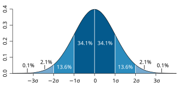
For the normal distribution, the values less than one standard deviation away from the mean account for 68.27% of the set; while two standard deviations from the mean account for 95.45%; and three standard deviations account for 99.73%.
About 68% of values drawn from a normal distribution are within one standard deviation σ away from the mean; about 95% of the values lie within two standard deviations; and about 99.7% are within three standard deviations.[5] This fact is known as the 68-95-99.7 (empirical) rule, or the 3-sigma rule.
More precisely, the probability that a normal deviate lies in the range between  and
and  is given by

To 12 significant digits, the values for  are:[citation needed]
 |
 |
 |
 |
OEIS | ||
|---|---|---|---|---|---|---|
| 1 | 0.682689492137 | 0.317310507863 |
|
OEIS: A178647 | ||
| 2 | 0.954499736104 | 0.045500263896 |
|
OEIS: A110894 | ||
| 3 | 0.997300203937 | 0.002699796063 |
|
OEIS: A270712 | ||
| 4 | 0.999936657516 | 0.000063342484 |
|
|||
| 5 | 0.999999426697 | 0.000000573303 |
|
|||
| 6 | 0.999999998027 | 0.000000001973 |
|
For large , one can use the approximation  .
.
Quantile function[edit]
The quantile function of a distribution is the inverse of the cumulative distribution function. The quantile function of the standard normal distribution is called the probit function, and can be expressed in terms of the inverse error function:

For a normal random variable with mean and variance , the quantile function is

The quantile  of the standard normal distribution is commonly denoted as
  . These values are used in hypothesis testing, construction of confidence intervals and Q–Q plots. A normal random variable will exceed
  with probability
  , and will lie outside the interval
  with probability
  . In particular, the quantile
  is 1.96; therefore a normal random variable will lie outside the interval
  in only 5% of cases.
The following table gives the quantile such that will lie in the range with a specified probability  . These values are useful to determine tolerance interval for sample averages and other statistical estimators with normal (or asymptotically normal) distributions.[citation needed] Note that the following table shows
  , not as defined above.
|
|
|
|
|
|---|---|---|---|---|
| 0.80 | 1.281551565545 | 0.999 | 3.290526731492 | |
| 0.90 | 1.644853626951 | 0.9999 | 3.890591886413 | |
| 0.95 | 1.959963984540 | 0.99999 | 4.417173413469 | |
| 0.98 | 2.326347874041 | 0.999999 | 4.891638475699 | |
| 0.99 | 2.575829303549 | 0.9999999 | 5.326723886384 | |
| 0.995 | 2.807033768344 | 0.99999999 | 5.730728868236 | |
| 0.998 | 3.090232306168 | 0.999999999 | 6.109410204869 |
For small , the quantile function has the useful asymptotic expansion
 [citation needed]
Properties[edit]
The normal distribution is the only distribution whose cumulants beyond the first two (i.e., other than the mean and variance) are zero. It is also the continuous distribution with the maximum entropy for a specified mean and variance.[14][15] Geary has shown, assuming that the mean and variance are finite, that the normal distribution is the only distribution where the mean and variance calculated from a set of independent draws are independent of each other.[16][17]
The normal distribution is a subclass of the elliptical distributions. The normal distribution is symmetric about its mean, and is non-zero over the entire real line. As such it may not be a suitable model for variables that are inherently positive or strongly skewed, such as the weight of a person or the price of a share. Such variables may be better described by other distributions, such as the log-normal distribution or the Pareto distribution.
The value of the normal distribution is practically zero when the value lies more than a few standard deviations away from the mean (e.g., a spread of three standard deviations covers all but 0.27% of the total distribution). Therefore, it may not be an appropriate model when one expects a significant fraction of outliers—values that lie many standard deviations away from the mean—and least squares and other statistical inference methods that are optimal for normally distributed variables often become highly unreliable when applied to such data. In those cases, a more heavy-tailed distribution should be assumed and the appropriate robust statistical inference methods applied.
The Gaussian distribution belongs to the family of stable distributions which are the attractors of sums of independent, identically distributed distributions whether or not the mean or variance is finite. Except for the Gaussian which is a limiting case, all stable distributions have heavy tails and infinite variance. It is one of the few distributions that are stable and that have probability density functions that can be expressed analytically, the others being the Cauchy distribution and the Lévy distribution.
Symmetries and derivatives[edit]
The normal distribution with density  (mean and standard deviation
  ) has the following properties:
Furthermore, the density of the standard normal distribution (i.e. and ) also has the following properties:
Moments[edit]
The plain and absolute moments of a variable are the expected values of  and
and  , respectively. If the expected value of is zero, these parameters are called central moments; otherwise, these parameters are called non-central moments. Usually we are interested only in moments with integer order
  .
.
If has a normal distribution, the non-central moments exist and are finite for any whose real part is greater than −1. For any non-negative integer , the plain central moments are:[21]
![{displaystyle operatorname {E} left[(X-mu )^{p}right]={begin{cases}0&{text{if }}p{text{ is odd,}}\sigma ^{p}(p-1)!!&{text{if }}p{text{ is even.}}end{cases}}}](https://wikimedia.org/api/rest_v1/media/math/render/svg/f1d2c92b62ac2bbe07a8e475faac29c8cc5f7755)
Here  denotes the double factorial, that is, the product of all numbers from to 1 that have the same parity as
The central absolute moments coincide with plain moments for all even orders, but are nonzero for odd orders. For any non-negative integer 
![{displaystyle {begin{aligned}operatorname {E} left[|X-mu |^{p}right]&=sigma ^{p}(p-1)!!cdot {begin{cases}{sqrt {frac {2}{pi }}}&{text{if }}p{text{ is odd}}\1&{text{if }}p{text{ is even}}end{cases}}\&=sigma ^{p}cdot {frac {2^{p/2}Gamma left({frac {p+1}{2}}right)}{sqrt {pi }}}.end{aligned}}}](https://wikimedia.org/api/rest_v1/media/math/render/svg/3b196371c491676efa7ea7770ef56773db7652cd)
The last formula is valid also for any non-integer  When the mean
  the plain and absolute moments can be expressed in terms of confluent hypergeometric functions
  and
and  [citation needed]
![{displaystyle {begin{aligned}operatorname {E} left[X^{p}right]&=sigma ^{p}cdot (-i{sqrt {2}})^{p}Uleft(-{frac {p}{2}},{frac {1}{2}},-{frac {1}{2}}left({frac {mu }{sigma }}right)^{2}right),\operatorname {E} left[|X|^{p}right]&=sigma ^{p}cdot 2^{p/2}{frac {Gamma left({frac {1+p}{2}}right)}{sqrt {pi }}}{}_{1}F_{1}left(-{frac {p}{2}},{frac {1}{2}},-{frac {1}{2}}left({frac {mu }{sigma }}right)^{2}right).end{aligned}}}](https://wikimedia.org/api/rest_v1/media/math/render/svg/0c17bf881593b86e728bf5dfbdb41a4b86da3875)
These expressions remain valid even if is not an integer. See also generalized Hermite polynomials.
| Order | Non-central moment | Central moment |
|---|---|---|
| 1 |
|
|
| 2 | 
|
|
| 3 | 
|
|
| 4 | 
|

|
| 5 | 
|
|
| 6 | 
|

|
| 7 | 
|
|
| 8 | 
|

|
The expectation of conditioned on the event that lies in an interval ![[a,b]](https://wikimedia.org/api/rest_v1/media/math/render/svg/9c4b788fc5c637e26ee98b45f89a5c08c85f7935) is given by
is given by
![{displaystyle operatorname {E} left[Xmid a<X<bright]=mu -sigma ^{2}{frac {f(b)-f(a)}{F(b)-F(a)}}}](https://wikimedia.org/api/rest_v1/media/math/render/svg/d82ec10bf31f0b63137699ae6e2b5a346770b097)
where and  respectively are the density and the cumulative distribution function of . For
  this is known as the inverse Mills ratio. Note that above, density of is used instead of standard normal density as in inverse Mills ratio, so here we have instead of .
Fourier transform and characteristic function[edit]
The Fourier transform of a normal density with mean and standard deviation is[22]

where  is the imaginary unit. If the mean , the first factor is 1, and the Fourier transform is, apart from a constant factor, a normal density on the frequency domain, with mean 0 and standard deviation . In particular, the standard normal distribution is an eigenfunction of the Fourier transform.
In probability theory, the Fourier transform of the probability distribution of a real-valued random variable is closely connected to the characteristic function  of that variable, which is defined as the expected value of
  , as a function of the real variable
  (the frequency parameter of the Fourier transform). This definition can be analytically extended to a complex-value variable .[23] The relation between both is:

Moment and cumulant generating functions[edit]
The moment generating function of a real random variable is the expected value of  , as a function of the real parameter . For a normal distribution with density , mean and deviation , the moment generating function exists and is equal to
![{displaystyle M(t)=operatorname {E} [e^{tX}]={hat {f}}(it)=e^{mu t}e^{{tfrac {1}{2}}sigma ^{2}t^{2}}}](https://wikimedia.org/api/rest_v1/media/math/render/svg/04bbd225c0fee5e58e9a8cd73b0f1b2bf535dc56)
The cumulant generating function is the logarithm of the moment generating function, namely

Since this is a quadratic polynomial in , only the first two cumulants are nonzero, namely the mean and the variance .
Stein operator and class[edit]
Within Stein’s method the Stein operator and class of a random variable  are
are  and
and  the class of all absolutely continuous functions
 ![{displaystyle f:mathbb {R} to mathbb {R} {mbox{ such that }}mathbb {E} [|f'(X)|]<infty }](https://wikimedia.org/api/rest_v1/media/math/render/svg/69d73a6b7e591a67eaff64aaf974a8c37584626e) .
.
Zero-variance limit[edit]
In the limit when tends to zero, the probability density eventually tends to zero at any  , but grows without limit if
  , while its integral remains equal to 1. Therefore, the normal distribution cannot be defined as an ordinary function when
  .
.
However, one can define the normal distribution with zero variance as a generalized function; specifically, as Dirac’s «delta function»  translated by the mean , that is
Its CDF is then the Heaviside step function translated by the mean , namely

Maximum entropy[edit]
Of all probability distributions over the reals with a specified mean and variance , the normal distribution is the one with maximum entropy.[24] If is a continuous random variable with probability density , then the entropy of is defined as[25][26][27]

where  is understood to be zero whenever
  . This functional can be maximized, subject to the constraints that the distribution is properly normalized and has a specified variance, by using variational calculus. A function with two Lagrange multipliers is defined:

where is, for now, regarded as some density function with mean and standard deviation .
At maximum entropy, a small variation  about will produce a variation
  about
about  which is equal to 0:

Since this must hold for any small , the term in brackets must be zero, and solving for yields:

Using the constraint equations to solve for  and
and  yields the density of the normal distribution:

The entropy of a normal distribution is equal to

Other properties[edit]
- If the characteristic function of some random variable is of the form , where is a polynomial, then the Marcinkiewicz theorem (named after Józef Marcinkiewicz) asserts that can be at most a quadratic polynomial, and therefore is a normal random variable.[28] The consequence of this result is that the normal distribution is the only distribution with a finite number (two) of non-zero cumulants.
- If and are jointly normal and uncorrelated, then they are independent. The requirement that and should be jointly normal is essential; without it the property does not hold.[29][30][proof] For non-normal random variables uncorrelatedness does not imply independence.
- The Kullback–Leibler divergence of one normal distribution from another is given by:[31]
The Hellinger distance between the same distributions is equal to
- The Fisher information matrix for a normal distribution w.r.t. and is diagonal and takes the form
- The conjugate prior of the mean of a normal distribution is another normal distribution.[32] Specifically, if are iid and the prior is , then the posterior distribution for the estimator of will be
- The family of normal distributions not only forms an exponential family (EF), but in fact forms a natural exponential family (NEF) with quadratic variance function (NEF-QVF). Many properties of normal distributions generalize to properties of NEF-QVF distributions, NEF distributions, or EF distributions generally. NEF-QVF distributions comprises 6 families, including Poisson, Gamma, binomial, and negative binomial distributions, while many of the common families studied in probability and statistics are NEF or EF.
- In information geometry, the family of normal distributions forms a statistical manifold with constant curvature . The same family is flat with respect to the (±1)-connections and .[33]


[edit]
Central limit theorem[edit]
As the number of discrete events increases, the function begins to resemble a normal distribution

Comparison of probability density functions,  for the sum of fair 6-sided dice to show their convergence to a normal distribution with increasing
  , in accordance to the central limit theorem. In the bottom-right graph, smoothed profiles of the previous graphs are rescaled, superimposed and compared with a normal distribution (black curve).
The central limit theorem states that under certain (fairly common) conditions, the sum of many random variables will have an approximately normal distribution. More specifically, where  are independent and identically distributed random variables with the same arbitrary distribution, zero mean, and variance and is their
mean scaled by 

Then, as increases, the probability distribution of will tend to the normal distribution with zero mean and variance .
The theorem can be extended to variables  that are not independent and/or not identically distributed if certain constraints are placed on the degree of dependence and the moments of the distributions.
Many test statistics, scores, and estimators encountered in practice contain sums of certain random variables in them, and even more estimators can be represented as sums of random variables through the use of influence functions. The central limit theorem implies that those statistical parameters will have asymptotically normal distributions.
The central limit theorem also implies that certain distributions can be approximated by the normal distribution, for example:
Whether these approximations are sufficiently accurate depends on the purpose for which they are needed, and the rate of convergence to the normal distribution. It is typically the case that such approximations are less accurate in the tails of the distribution.
A general upper bound for the approximation error in the central limit theorem is given by the Berry–Esseen theorem, improvements of the approximation are given by the Edgeworth expansions.
This theorem can also be used to justify modeling the sum of many uniform noise sources as Gaussian noise. See AWGN.
Operations and functions of normal variables[edit]

a: Probability density of a function  of a normal variable with
  and
and  . b: Probability density of a function
  of two normal variables and
  , where
  ,
,  ,
,  ,
,  , and
, and  . c: Heat map of the joint probability density of two functions of two correlated normal variables and , where
  ,
,  ,
,  ,
,  , and
, and  . d: Probability density of a function
  of 4 iid standard normal variables. These are computed by the numerical method of ray-tracing.[35]
The probability density, cumulative distribution, and inverse cumulative distribution of any function of one or more independent or correlated normal variables can be computed with the numerical method of ray-tracing[35] (Matlab code). In the following sections we look at some special cases.
Operations on a single normal variable[edit]
If is distributed normally with mean and variance , then
- , for any real numbers and , is also normally distributed, with mean and standard deviation . That is, the family of normal distributions is closed under linear transformations.
- The exponential of is distributed log-normally: eX ~ ln(N (μ, σ2)).
- The absolute value of has folded normal distribution: |X| ~ Nf (μ, σ2). If this is known as the half-normal distribution.
- The absolute value of normalized residuals, |X − μ|/σ, has chi distribution with one degree of freedom: .
- The square of X/σ has the noncentral chi-squared distribution with one degree of freedom: . If , the distribution is called simply chi-squared.
- The log-likelihood of a normal variable is simply the log of its probability density function:
Since this is a scaled and shifted square of a standard normal variable, it is distributed as a scaled and shifted chi-squared variable.
- The distribution of the variable X restricted to an interval [a, b] is called the truncated normal distribution.
- (X − μ)−2 has a Lévy distribution with location 0 and scale σ−2.


Operations on two independent normal variables[edit]
- If and are two independent normal random variables, with means , and standard deviations , , then their sum will also be normally distributed,[proof] with mean and variance .
- In particular, if and are independent normal deviates with zero mean and variance , then and are also independent and normally distributed, with zero mean and variance . This is a special case of the polarization identity.[36]
- If , are two independent normal deviates with mean and deviation , and , are arbitrary real numbers, then the variable
is also normally distributed with mean
and deviation . It follows that the normal distribution is stable (with exponent ).


Operations on two independent standard normal variables[edit]
If  and
and  are two independent standard normal random variables with mean 0 and variance 1, then
Operations on multiple independent normal variables[edit]
[edit]
- A quadratic form of a normal vector, i.e. a quadratic function of multiple independent or correlated normal variables, is a generalized chi-square variable.

Operations on the density function[edit]
The split normal distribution is most directly defined in terms of joining scaled sections of the density functions of different normal distributions and rescaling the density to integrate to one. The truncated normal distribution results from rescaling a section of a single density function.
Infinite divisibility and Cramér’s theorem[edit]
For any positive integer  , any normal distribution with mean and variance is the distribution of the sum of independent normal deviates, each with mean
  and variance
  . This property is called infinite divisibility.[41]
Conversely, if and are independent random variables and their sum  has a normal distribution, then both and must be normal deviates.[42]
This result is known as Cramér’s decomposition theorem, and is equivalent to saying that the convolution of two distributions is normal if and only if both are normal. Cramér’s theorem implies that a linear combination of independent non-Gaussian variables will never have an exactly normal distribution, although it may approach it arbitrarily closely.[28]
Bernstein’s theorem[edit]
Bernstein’s theorem states that if and  are independent and
  and
and  are also independent, then both X and Y must necessarily have normal distributions.[43][44]
More generally, if are independent random variables, then two distinct linear combinations  and
and  will be independent if and only if all
  are normal and
  , where
  denotes the variance of .[43]
Extensions[edit]
The notion of normal distribution, being one of the most important distributions in probability theory, has been extended far beyond the standard framework of the univariate (that is one-dimensional) case (Case 1). All these extensions are also called normal or Gaussian laws, so a certain ambiguity in names exists.
- The multivariate normal distribution describes the Gaussian law in the k-dimensional Euclidean space. A vector X ∈ Rk is multivariate-normally distributed if any linear combination of its components Σk
j=1aj Xj has a (univariate) normal distribution. The variance of X is a k×k symmetric positive-definite matrix V. The multivariate normal distribution is a special case of the elliptical distributions. As such, its iso-density loci in the k = 2 case are ellipses and in the case of arbitrary k are ellipsoids. - Rectified Gaussian distribution a rectified version of normal distribution with all the negative elements reset to 0
- Complex normal distribution deals with the complex normal vectors. A complex vector X ∈ Ck is said to be normal if both its real and imaginary components jointly possess a 2k-dimensional multivariate normal distribution. The variance-covariance structure of X is described by two matrices: the variance matrix Γ, and the relation matrix C.
- Matrix normal distribution describes the case of normally distributed matrices.
- Gaussian processes are the normally distributed stochastic processes. These can be viewed as elements of some infinite-dimensional Hilbert space H, and thus are the analogues of multivariate normal vectors for the case k = ∞. A random element h ∈ H is said to be normal if for any constant a ∈ H the scalar product (a, h) has a (univariate) normal distribution. The variance structure of such Gaussian random element can be described in terms of the linear covariance operator K: H → H. Several Gaussian processes became popular enough to have their own names:
- Brownian motion,
- Brownian bridge,
- Ornstein–Uhlenbeck process.
- Gaussian q-distribution is an abstract mathematical construction that represents a «q-analogue» of the normal distribution.
- the q-Gaussian is an analogue of the Gaussian distribution, in the sense that it maximises the Tsallis entropy, and is one type of Tsallis distribution. Note that this distribution is different from the Gaussian q-distribution above.
- The Kaniadakis κ-Gaussian distribution is a generalization of the Gaussian distribution which arises from the Kaniadakis statistics, being one of the Kaniadakis distributions.
A random variable X has a two-piece normal distribution if it has a distribution


where μ is the mean and σ1 and σ2 are the standard deviations of the distribution to the left and right of the mean respectively.
The mean, variance and third central moment of this distribution have been determined[45]


![{displaystyle operatorname {T} (X)={sqrt {frac {2}{pi }}}(sigma _{2}-sigma _{1})left[left({frac {4}{pi }}-1right)(sigma _{2}-sigma _{1})^{2}+sigma _{1}sigma _{2}right]}](https://wikimedia.org/api/rest_v1/media/math/render/svg/9959f2c5186e2ed76884054edaf837a602ac6fac)
where E(X), V(X) and T(X) are the mean, variance, and third central moment respectively.
One of the main practical uses of the Gaussian law is to model the empirical distributions of many different random variables encountered in practice. In such case a possible extension would be a richer family of distributions, having more than two parameters and therefore being able to fit the empirical distribution more accurately. The examples of such extensions are:
- Pearson distribution — a four-parameter family of probability distributions that extend the normal law to include different skewness and kurtosis values.
- The generalized normal distribution, also known as the exponential power distribution, allows for distribution tails with thicker or thinner asymptotic behaviors.
Statistical inference[edit]
Estimation of parameters[edit]
It is often the case that we do not know the parameters of the normal distribution, but instead want to estimate them. That is, having a sample  from a normal population we would like to learn the approximate values of parameters and . The standard approach to this problem is the maximum likelihood method, which requires maximization of the log-likelihood function:

Taking derivatives with respect to and and solving the resulting system of first order conditions yields the maximum likelihood estimates:

Sample mean[edit]
Estimator  is called the sample mean, since it is the arithmetic mean of all observations. The statistic
  is complete and sufficient for , and therefore by the Lehmann–Scheffé theorem, is the uniformly minimum variance unbiased (UMVU) estimator.[46] In finite samples it is distributed normally:

The variance of this estimator is equal to the μμ-element of the inverse Fisher information matrix  . This implies that the estimator is finite-sample efficient. Of practical importance is the fact that the standard error of is proportional to
  , that is, if one wishes to decrease the standard error by a factor of 10, one must increase the number of points in the sample by a factor of 100. This fact is widely used in determining sample sizes for opinion polls and the number of trials in Monte Carlo simulations.
From the standpoint of the asymptotic theory, is consistent, that is, it converges in probability to as  . The estimator is also asymptotically normal, which is a simple corollary of the fact that it is normal in finite samples:

Sample variance[edit]
The estimator  is called the sample variance, since it is the variance of the sample (). In practice, another estimator is often used instead of the . This other estimator is denoted
  , and is also called the sample variance, which represents a certain ambiguity in terminology; its square root
  is called the sample standard deviation. The estimator differs from by having (n − 1) instead of n in the denominator (the so-called Bessel’s correction):

The difference between and becomes negligibly small for large n‘s. In finite samples however, the motivation behind the use of is that it is an unbiased estimator of the underlying parameter , whereas is biased. Also, by the Lehmann–Scheffé theorem the estimator is uniformly minimum variance unbiased (UMVU),[46] which makes it the «best» estimator among all unbiased ones. However it can be shown that the biased estimator is «better» than the in terms of the mean squared error (MSE) criterion. In finite samples both and have scaled chi-squared distribution with (n − 1) degrees of freedom:

The first of these expressions shows that the variance of is equal to  , which is slightly greater than the σσ-element of the inverse Fisher information matrix . Thus, is not an efficient estimator for , and moreover, since is UMVU, we can conclude that the finite-sample efficient estimator for does not exist.
Applying the asymptotic theory, both estimators and are consistent, that is they converge in probability to as the sample size . The two estimators are also both asymptotically normal:

In particular, both estimators are asymptotically efficient for .
Confidence intervals[edit]
By Cochran’s theorem, for normal distributions the sample mean and the sample variance s2 are independent, which means there can be no gain in considering their joint distribution. There is also a converse theorem: if in a sample the sample mean and sample variance are independent, then the sample must have come from the normal distribution. The independence between and s can be employed to construct the so-called t-statistic:

This quantity t has the Student’s t-distribution with (n − 1) degrees of freedom, and it is an ancillary statistic (independent of the value of the parameters). Inverting the distribution of this t-statistics will allow us to construct the confidence interval for μ;[47] similarly, inverting the χ2 distribution of the statistic s2 will give us the confidence interval for σ2:[48]
![{displaystyle mu in left[{hat {mu }}-t_{n-1,1-alpha /2}{frac {1}{sqrt {n}}}s,{hat {mu }}+t_{n-1,1-alpha /2}{frac {1}{sqrt {n}}}sright],}](https://wikimedia.org/api/rest_v1/media/math/render/svg/f6e3068587bfbaf61a549a39b518757119bfb846)
![{displaystyle sigma ^{2}in left[{frac {(n-1)s^{2}}{chi _{n-1,1-alpha /2}^{2}}},{frac {(n-1)s^{2}}{chi _{n-1,alpha /2}^{2}}}right],}](https://wikimedia.org/api/rest_v1/media/math/render/svg/3549a31cb861d9e479c232271cb88b019cfa9fd5)
where tk,p and χ 2
k,p are the pth quantiles of the t— and χ2-distributions respectively. These confidence intervals are of the confidence level 1 − α, meaning that the true values μ and σ2 fall outside of these intervals with probability (or significance level) α. In practice people usually take α = 5%, resulting in the 95% confidence intervals.
Approximate formulas can be derived from the asymptotic distributions of and s2:
![{displaystyle mu in left[{hat {mu }}-|z_{alpha /2}|{frac {1}{sqrt {n}}}s,{hat {mu }}+|z_{alpha /2}|{frac {1}{sqrt {n}}}sright],}](https://wikimedia.org/api/rest_v1/media/math/render/svg/e13883f93c0a1405e71bd105685ecac6b4c84089)
![{displaystyle sigma ^{2}in left[s^{2}-|z_{alpha /2}|{frac {sqrt {2}}{sqrt {n}}}s^{2},s^{2}+|z_{alpha /2}|{frac {sqrt {2}}{sqrt {n}}}s^{2}right],}](https://wikimedia.org/api/rest_v1/media/math/render/svg/e3e7c940eb3f6f50af62200ae75e10435ef8dfe6)
The approximate formulas become valid for large values of n, and are more convenient for the manual calculation since the standard normal quantiles zα/2 do not depend on n. In particular, the most popular value of α = 5%, results in |z0.025| = 1.96.
Normality tests[edit]
Normality tests assess the likelihood that the given data set {x1, …, xn} comes from a normal distribution. Typically the null hypothesis H0 is that the observations are distributed normally with unspecified mean μ and variance σ2, versus the alternative Ha that the distribution is arbitrary. Many tests (over 40) have been devised for this problem. The more prominent of them are outlined below:
Diagnostic plots are more intuitively appealing but subjective at the same time, as they rely on informal human judgement to accept or reject the null hypothesis.
- Q–Q plot, also known as normal probability plot or rankit plot—is a plot of the sorted values from the data set against the expected values of the corresponding quantiles from the standard normal distribution. That is, it’s a plot of point of the form (Φ−1(pk), x(k)), where plotting points pk are equal to pk = (k − α)/(n + 1 − 2α) and α is an adjustment constant, which can be anything between 0 and 1. If the null hypothesis is true, the plotted points should approximately lie on a straight line.
- P–P plot – similar to the Q–Q plot, but used much less frequently. This method consists of plotting the points (Φ(z(k)), pk), where . For normally distributed data this plot should lie on a 45° line between (0, 0) and (1, 1).

Goodness-of-fit tests:
Moment-based tests:
- D’Agostino’s K-squared test
- Jarque–Bera test
- Shapiro–Wilk test: This is based on the fact that the line in the Q–Q plot has the slope of σ. The test compares the least squares estimate of that slope with the value of the sample variance, and rejects the null hypothesis if these two quantities differ significantly.
Tests based on the empirical distribution function:
- Anderson–Darling test
- Lilliefors test (an adaptation of the Kolmogorov–Smirnov test)
Bayesian analysis of the normal distribution[edit]
Bayesian analysis of normally distributed data is complicated by the many different possibilities that may be considered:
- Either the mean, or the variance, or neither, may be considered a fixed quantity.
- When the variance is unknown, analysis may be done directly in terms of the variance, or in terms of the precision, the reciprocal of the variance. The reason for expressing the formulas in terms of precision is that the analysis of most cases is simplified.
- Both univariate and multivariate cases need to be considered.
- Either conjugate or improper prior distributions may be placed on the unknown variables.
- An additional set of cases occurs in Bayesian linear regression, where in the basic model the data is assumed to be normally distributed, and normal priors are placed on the regression coefficients. The resulting analysis is similar to the basic cases of independent identically distributed data.
The formulas for the non-linear-regression cases are summarized in the conjugate prior article.
Sum of two quadratics[edit]
Scalar form[edit]
The following auxiliary formula is useful for simplifying the posterior update equations, which otherwise become fairly tedious.

This equation rewrites the sum of two quadratics in x by expanding the squares, grouping the terms in x, and completing the square. Note the following about the complex constant factors attached to some of the terms:
- The factor has the form of a weighted average of y and z.
- This shows that this factor can be thought of as resulting from a situation where the reciprocals of quantities a and b add directly, so to combine a and b themselves, it’s necessary to reciprocate, add, and reciprocate the result again to get back into the original units. This is exactly the sort of operation performed by the harmonic mean, so it is not surprising that is one-half the harmonic mean of a and b.


Vector form[edit]
A similar formula can be written for the sum of two vector quadratics: If x, y, z are vectors of length k, and A and B are symmetric, invertible matrices of size  , then

where

Note that the form x′ A x is called a quadratic form and is a scalar:

In other words, it sums up all possible combinations of products of pairs of elements from x, with a separate coefficient for each. In addition, since  , only the sum
  matters for any off-diagonal elements of A, and there is no loss of generality in assuming that A is symmetric. Furthermore, if A is symmetric, then the form
Sum of differences from the mean[edit]
Another useful formula is as follows:

where 
With known variance[edit]
For a set of i.i.d. normally distributed data points X of size n where each individual point x follows  with known variance σ2, the conjugate prior distribution is also normally distributed.
This can be shown more easily by rewriting the variance as the precision, i.e. using τ = 1/σ2. Then if  and
and  we proceed as follows.
First, the likelihood function is (using the formula above for the sum of differences from the mean):
![{displaystyle {begin{aligned}p(mathbf {X} mid mu ,tau )&=prod _{i=1}^{n}{sqrt {frac {tau }{2pi }}}exp left(-{frac {1}{2}}tau (x_{i}-mu )^{2}right)\&=left({frac {tau }{2pi }}right)^{n/2}exp left(-{frac {1}{2}}tau sum _{i=1}^{n}(x_{i}-mu )^{2}right)\&=left({frac {tau }{2pi }}right)^{n/2}exp left[-{frac {1}{2}}tau left(sum _{i=1}^{n}(x_{i}-{bar {x}})^{2}+n({bar {x}}-mu )^{2}right)right].end{aligned}}}](https://wikimedia.org/api/rest_v1/media/math/render/svg/c2bcd1c34520a24e29b758a0f7427e79e9d8a414)
Then, we proceed as follows:
![{displaystyle {begin{aligned}p(mu mid mathbf {X} )&propto p(mathbf {X} mid mu )p(mu )\&=left({frac {tau }{2pi }}right)^{n/2}exp left[-{frac {1}{2}}tau left(sum _{i=1}^{n}(x_{i}-{bar {x}})^{2}+n({bar {x}}-mu )^{2}right)right]{sqrt {frac {tau _{0}}{2pi }}}exp left(-{frac {1}{2}}tau _{0}(mu -mu _{0})^{2}right)\&propto exp left(-{frac {1}{2}}left(tau left(sum _{i=1}^{n}(x_{i}-{bar {x}})^{2}+n({bar {x}}-mu )^{2}right)+tau _{0}(mu -mu _{0})^{2}right)right)\&propto exp left(-{frac {1}{2}}left(ntau ({bar {x}}-mu )^{2}+tau _{0}(mu -mu _{0})^{2}right)right)\&=exp left(-{frac {1}{2}}(ntau +tau _{0})left(mu -{dfrac {ntau {bar {x}}+tau _{0}mu _{0}}{ntau +tau _{0}}}right)^{2}+{frac {ntau tau _{0}}{ntau +tau _{0}}}({bar {x}}-mu _{0})^{2}right)\&propto exp left(-{frac {1}{2}}(ntau +tau _{0})left(mu -{dfrac {ntau {bar {x}}+tau _{0}mu _{0}}{ntau +tau _{0}}}right)^{2}right)end{aligned}}}](https://wikimedia.org/api/rest_v1/media/math/render/svg/96e309ead00fbc8603eced5342aa5df534522d6a)
In the above derivation, we used the formula above for the sum of two quadratics and eliminated all constant factors not involving μ. The result is the kernel of a normal distribution, with mean  and precision
  , i.e.

This can be written as a set of Bayesian update equations for the posterior parameters in terms of the prior parameters:
![{displaystyle {begin{aligned}tau _{0}'&=tau _{0}+ntau \[5pt]mu _{0}'&={frac {ntau {bar {x}}+tau _{0}mu _{0}}{ntau +tau _{0}}}\[5pt]{bar {x}}&={frac {1}{n}}sum _{i=1}^{n}x_{i}end{aligned}}}](https://wikimedia.org/api/rest_v1/media/math/render/svg/a6cfbdf504b1a9ce4cbe79561b4ae983fdf7271d)
That is, to combine n data points with total precision of nτ (or equivalently, total variance of n/σ2) and mean of values  , derive a new total precision simply by adding the total precision of the data to the prior total precision, and form a new mean through a precision-weighted average, i.e. a weighted average of the data mean and the prior mean, each weighted by the associated total precision. This makes logical sense if the precision is thought of as indicating the certainty of the observations: In the distribution of the posterior mean, each of the input components is weighted by its certainty, and the certainty of this distribution is the sum of the individual certainties. (For the intuition of this, compare the expression «the whole is (or is not) greater than the sum of its parts». In addition, consider that the knowledge of the posterior comes from a combination of the knowledge of the prior and likelihood, so it makes sense that we are more certain of it than of either of its components.)
The above formula reveals why it is more convenient to do Bayesian analysis of conjugate priors for the normal distribution in terms of the precision. The posterior precision is simply the sum of the prior and likelihood precisions, and the posterior mean is computed through a precision-weighted average, as described above. The same formulas can be written in terms of variance by reciprocating all the precisions, yielding the more ugly formulas
![{displaystyle {begin{aligned}{sigma _{0}^{2}}'&={frac {1}{{frac {n}{sigma ^{2}}}+{frac {1}{sigma _{0}^{2}}}}}\[5pt]mu _{0}'&={frac {{frac {n{bar {x}}}{sigma ^{2}}}+{frac {mu _{0}}{sigma _{0}^{2}}}}{{frac {n}{sigma ^{2}}}+{frac {1}{sigma _{0}^{2}}}}}\[5pt]{bar {x}}&={frac {1}{n}}sum _{i=1}^{n}x_{i}end{aligned}}}](https://wikimedia.org/api/rest_v1/media/math/render/svg/ea454c8840683777ce8192d9ae63068c63962858)
With known mean[edit]
For a set of i.i.d. normally distributed data points X of size n where each individual point x follows with known mean μ, the conjugate prior of the variance has an inverse gamma distribution or a scaled inverse chi-squared distribution. The two are equivalent except for having different parameterizations. Although the inverse gamma is more commonly used, we use the scaled inverse chi-squared for the sake of convenience. The prior for σ2 is as follows:
![{displaystyle p(sigma ^{2}mid nu _{0},sigma _{0}^{2})={frac {(sigma _{0}^{2}{frac {nu _{0}}{2}})^{nu _{0}/2}}{Gamma left({frac {nu _{0}}{2}}right)}}~{frac {exp left[{frac {-nu _{0}sigma _{0}^{2}}{2sigma ^{2}}}right]}{(sigma ^{2})^{1+{frac {nu _{0}}{2}}}}}propto {frac {exp left[{frac {-nu _{0}sigma _{0}^{2}}{2sigma ^{2}}}right]}{(sigma ^{2})^{1+{frac {nu _{0}}{2}}}}}}](https://wikimedia.org/api/rest_v1/media/math/render/svg/ef2528fe4774a93087d4adae570ef9ab84707f52)
The likelihood function from above, written in terms of the variance, is:
![{displaystyle {begin{aligned}p(mathbf {X} mid mu ,sigma ^{2})&=left({frac {1}{2pi sigma ^{2}}}right)^{n/2}exp left[-{frac {1}{2sigma ^{2}}}sum _{i=1}^{n}(x_{i}-mu )^{2}right]\&=left({frac {1}{2pi sigma ^{2}}}right)^{n/2}exp left[-{frac {S}{2sigma ^{2}}}right]end{aligned}}}](https://wikimedia.org/api/rest_v1/media/math/render/svg/cc06aa31588bba03e4748f8f345f0638a75dc156)
where

Then:
![{displaystyle {begin{aligned}p(sigma ^{2}mid mathbf {X} )&propto p(mathbf {X} mid sigma ^{2})p(sigma ^{2})\&=left({frac {1}{2pi sigma ^{2}}}right)^{n/2}exp left[-{frac {S}{2sigma ^{2}}}right]{frac {(sigma _{0}^{2}{frac {nu _{0}}{2}})^{frac {nu _{0}}{2}}}{Gamma left({frac {nu _{0}}{2}}right)}}~{frac {exp left[{frac {-nu _{0}sigma _{0}^{2}}{2sigma ^{2}}}right]}{(sigma ^{2})^{1+{frac {nu _{0}}{2}}}}}\&propto left({frac {1}{sigma ^{2}}}right)^{n/2}{frac {1}{(sigma ^{2})^{1+{frac {nu _{0}}{2}}}}}exp left[-{frac {S}{2sigma ^{2}}}+{frac {-nu _{0}sigma _{0}^{2}}{2sigma ^{2}}}right]\&={frac {1}{(sigma ^{2})^{1+{frac {nu _{0}+n}{2}}}}}exp left[-{frac {nu _{0}sigma _{0}^{2}+S}{2sigma ^{2}}}right]end{aligned}}}](https://wikimedia.org/api/rest_v1/media/math/render/svg/381c1b93f6dc76e2cdca9f3f1f77132dd51dc55f)
The above is also a scaled inverse chi-squared distribution where

or equivalently

Reparameterizing in terms of an inverse gamma distribution, the result is:

With unknown mean and unknown variance[edit]
For a set of i.i.d. normally distributed data points X of size n where each individual point x follows with unknown mean μ and unknown variance σ2, a combined (multivariate) conjugate prior is placed over the mean and variance, consisting of a normal-inverse-gamma distribution.
Logically, this originates as follows:
- From the analysis of the case with unknown mean but known variance, we see that the update equations involve sufficient statistics computed from the data consisting of the mean of the data points and the total variance of the data points, computed in turn from the known variance divided by the number of data points.
- From the analysis of the case with unknown variance but known mean, we see that the update equations involve sufficient statistics over the data consisting of the number of data points and sum of squared deviations.
- Keep in mind that the posterior update values serve as the prior distribution when further data is handled. Thus, we should logically think of our priors in terms of the sufficient statistics just described, with the same semantics kept in mind as much as possible.
- To handle the case where both mean and variance are unknown, we could place independent priors over the mean and variance, with fixed estimates of the average mean, total variance, number of data points used to compute the variance prior, and sum of squared deviations. Note however that in reality, the total variance of the mean depends on the unknown variance, and the sum of squared deviations that goes into the variance prior (appears to) depend on the unknown mean. In practice, the latter dependence is relatively unimportant: Shifting the actual mean shifts the generated points by an equal amount, and on average the squared deviations will remain the same. This is not the case, however, with the total variance of the mean: As the unknown variance increases, the total variance of the mean will increase proportionately, and we would like to capture this dependence.
- This suggests that we create a conditional prior of the mean on the unknown variance, with a hyperparameter specifying the mean of the pseudo-observations associated with the prior, and another parameter specifying the number of pseudo-observations. This number serves as a scaling parameter on the variance, making it possible to control the overall variance of the mean relative to the actual variance parameter. The prior for the variance also has two hyperparameters, one specifying the sum of squared deviations of the pseudo-observations associated with the prior, and another specifying once again the number of pseudo-observations. Note that each of the priors has a hyperparameter specifying the number of pseudo-observations, and in each case this controls the relative variance of that prior. These are given as two separate hyperparameters so that the variance (aka the confidence) of the two priors can be controlled separately.
- This leads immediately to the normal-inverse-gamma distribution, which is the product of the two distributions just defined, with conjugate priors used (an inverse gamma distribution over the variance, and a normal distribution over the mean, conditional on the variance) and with the same four parameters just defined.
The priors are normally defined as follows:

The update equations can be derived, and look as follows:

The respective numbers of pseudo-observations add the number of actual observations to them. The new mean hyperparameter is once again a weighted average, this time weighted by the relative numbers of observations. Finally, the update for  is similar to the case with known mean, but in this case the sum of squared deviations is taken with respect to the observed data mean rather than the true mean, and as a result a new «interaction term» needs to be added to take care of the additional error source stemming from the deviation between prior and data mean.
Proof
The prior distributions are
![{displaystyle {begin{aligned}p(mu mid sigma ^{2};mu _{0},n_{0})&sim {mathcal {N}}(mu _{0},sigma ^{2}/n_{0})={frac {1}{sqrt {2pi {frac {sigma ^{2}}{n_{0}}}}}}exp left(-{frac {n_{0}}{2sigma ^{2}}}(mu -mu _{0})^{2}right)\&propto (sigma ^{2})^{-1/2}exp left(-{frac {n_{0}}{2sigma ^{2}}}(mu -mu _{0})^{2}right)\p(sigma ^{2};nu _{0},sigma _{0}^{2})&sim Ichi ^{2}(nu _{0},sigma _{0}^{2})=IG(nu _{0}/2,nu _{0}sigma _{0}^{2}/2)\&={frac {(sigma _{0}^{2}nu _{0}/2)^{nu _{0}/2}}{Gamma (nu _{0}/2)}}~{frac {exp left[{frac {-nu _{0}sigma _{0}^{2}}{2sigma ^{2}}}right]}{(sigma ^{2})^{1+nu _{0}/2}}}\&propto {(sigma ^{2})^{-(1+nu _{0}/2)}}exp left[{frac {-nu _{0}sigma _{0}^{2}}{2sigma ^{2}}}right].end{aligned}}}](https://wikimedia.org/api/rest_v1/media/math/render/svg/cf7afb8e3b63fb1526171840344b32458e55cf8b)
Therefore, the joint prior is
![{displaystyle {begin{aligned}p(mu ,sigma ^{2};mu _{0},n_{0},nu _{0},sigma _{0}^{2})&=p(mu mid sigma ^{2};mu _{0},n_{0}),p(sigma ^{2};nu _{0},sigma _{0}^{2})\&propto (sigma ^{2})^{-(nu _{0}+3)/2}exp left[-{frac {1}{2sigma ^{2}}}left(nu _{0}sigma _{0}^{2}+n_{0}(mu -mu _{0})^{2}right)right].end{aligned}}}](https://wikimedia.org/api/rest_v1/media/math/render/svg/b6f808161077baef3854dbfd90b870698d721090)
The likelihood function from the section above with known variance is:
![{begin{aligned}p(mathbf {X} mid mu ,sigma ^{2})&=left({frac {1}{2pi sigma ^{2}}}right)^{n/2}exp left[-{frac {1}{2sigma ^{2}}}left(sum _{i=1}^{n}(x_{i}-mu )^{2}right)right]end{aligned}}](https://wikimedia.org/api/rest_v1/media/math/render/svg/f3d77342aadcb34c5d84418cecaefdb52842b6b7)
Writing it in terms of variance rather than precision, we get:
![{begin{aligned}p(mathbf {X} mid mu ,sigma ^{2})&=left({frac {1}{2pi sigma ^{2}}}right)^{n/2}exp left[-{frac {1}{2sigma ^{2}}}left(sum _{i=1}^{n}(x_{i}-{bar {x}})^{2}+n({bar {x}}-mu )^{2}right)right]\&propto {sigma ^{2}}^{-n/2}exp left[-{frac {1}{2sigma ^{2}}}left(S+n({bar {x}}-mu )^{2}right)right]end{aligned}}](https://wikimedia.org/api/rest_v1/media/math/render/svg/29b915f070b522a1e9f419be05624c86c854ca14)
where 
Therefore, the posterior is (dropping the hyperparameters as conditioning factors):
![{begin{aligned}p(mu ,sigma ^{2}mid mathbf {X} )&propto p(mu ,sigma ^{2}),p(mathbf {X} mid mu ,sigma ^{2})\&propto (sigma ^{2})^{-(nu _{0}+3)/2}exp left[-{frac {1}{2sigma ^{2}}}left(nu _{0}sigma _{0}^{2}+n_{0}(mu -mu _{0})^{2}right)right]{sigma ^{2}}^{-n/2}exp left[-{frac {1}{2sigma ^{2}}}left(S+n({bar {x}}-mu )^{2}right)right]\&=(sigma ^{2})^{-(nu _{0}+n+3)/2}exp left[-{frac {1}{2sigma ^{2}}}left(nu _{0}sigma _{0}^{2}+S+n_{0}(mu -mu _{0})^{2}+n({bar {x}}-mu )^{2}right)right]\&=(sigma ^{2})^{-(nu _{0}+n+3)/2}exp left[-{frac {1}{2sigma ^{2}}}left(nu _{0}sigma _{0}^{2}+S+{frac {n_{0}n}{n_{0}+n}}(mu _{0}-{bar {x}})^{2}+(n_{0}+n)left(mu -{frac {n_{0}mu _{0}+n{bar {x}}}{n_{0}+n}}right)^{2}right)right]\&propto (sigma ^{2})^{-1/2}exp left[-{frac {n_{0}+n}{2sigma ^{2}}}left(mu -{frac {n_{0}mu _{0}+n{bar {x}}}{n_{0}+n}}right)^{2}right]\&quad times (sigma ^{2})^{-(nu _{0}/2+n/2+1)}exp left[-{frac {1}{2sigma ^{2}}}left(nu _{0}sigma _{0}^{2}+S+{frac {n_{0}n}{n_{0}+n}}(mu _{0}-{bar {x}})^{2}right)right]\&={mathcal {N}}_{mu mid sigma ^{2}}left({frac {n_{0}mu _{0}+n{bar {x}}}{n_{0}+n}},{frac {sigma ^{2}}{n_{0}+n}}right)cdot {rm {IG}}_{sigma ^{2}}left({frac {1}{2}}(nu _{0}+n),{frac {1}{2}}left(nu _{0}sigma _{0}^{2}+S+{frac {n_{0}n}{n_{0}+n}}(mu _{0}-{bar {x}})^{2}right)right).end{aligned}}](https://wikimedia.org/api/rest_v1/media/math/render/svg/cad9489034d77d53c12c7ee6044f712cfdb77831)
In other words, the posterior distribution has the form of a product of a normal distribution over p(μ | σ2) times an inverse gamma distribution over p(σ2), with parameters that are the same as the update equations above.
Occurrence and applications[edit]
The occurrence of normal distribution in practical problems can be loosely classified into four categories:
- Exactly normal distributions;
- Approximately normal laws, for example when such approximation is justified by the central limit theorem; and
- Distributions modeled as normal – the normal distribution being the distribution with maximum entropy for a given mean and variance.
- Regression problems – the normal distribution being found after systematic effects have been modeled sufficiently well.
Exact normality[edit]

Certain quantities in physics are distributed normally, as was first demonstrated by James Clerk Maxwell. Examples of such quantities are:
Approximate normality[edit]
Approximately normal distributions occur in many situations, as explained by the central limit theorem. When the outcome is produced by many small effects acting additively and independently, its distribution will be close to normal. The normal approximation will not be valid if the effects act multiplicatively (instead of additively), or if there is a single external influence that has a considerably larger magnitude than the rest of the effects.
- In counting problems, where the central limit theorem includes a discrete-to-continuum approximation and where infinitely divisible and decomposable distributions are involved, such as
- Binomial random variables, associated with binary response variables;
- Poisson random variables, associated with rare events;
- Thermal radiation has a Bose–Einstein distribution on very short time scales, and a normal distribution on longer timescales due to the central limit theorem.
Assumed normality[edit]
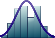
Histogram of sepal widths for Iris versicolor from Fisher’s Iris flower data set, with superimposed best-fitting normal distribution.
I can only recognize the occurrence of the normal curve – the Laplacian curve of errors – as a very abnormal phenomenon. It is roughly approximated to in certain distributions; for this reason, and on account for its beautiful simplicity, we may, perhaps, use it as a first approximation, particularly in theoretical investigations.
There are statistical methods to empirically test that assumption; see the above Normality tests section.
- In biology, the logarithm of various variables tend to have a normal distribution, that is, they tend to have a log-normal distribution (after separation on male/female subpopulations), with examples including:
- Measures of size of living tissue (length, height, skin area, weight);[49]
- The length of inert appendages (hair, claws, nails, teeth) of biological specimens, in the direction of growth; presumably the thickness of tree bark also falls under this category;
- Certain physiological measurements, such as blood pressure of adult humans.
- In finance, in particular the Black–Scholes model, changes in the logarithm of exchange rates, price indices, and stock market indices are assumed normal (these variables behave like compound interest, not like simple interest, and so are multiplicative). Some mathematicians such as Benoit Mandelbrot have argued that log-Levy distributions, which possesses heavy tails would be a more appropriate model, in particular for the analysis for stock market crashes. The use of the assumption of normal distribution occurring in financial models has also been criticized by Nassim Nicholas Taleb in his works.
- Measurement errors in physical experiments are often modeled by a normal distribution. This use of a normal distribution does not imply that one is assuming the measurement errors are normally distributed, rather using the normal distribution produces the most conservative predictions possible given only knowledge about the mean and variance of the errors.[50]
- In standardized testing, results can be made to have a normal distribution by either selecting the number and difficulty of questions (as in the IQ test) or transforming the raw test scores into «output» scores by fitting them to the normal distribution. For example, the SAT’s traditional range of 200–800 is based on a normal distribution with a mean of 500 and a standard deviation of 100.

- Many scores are derived from the normal distribution, including percentile ranks («percentiles» or «quantiles»), normal curve equivalents, stanines, z-scores, and T-scores. Additionally, some behavioral statistical procedures assume that scores are normally distributed; for example, t-tests and ANOVAs. Bell curve grading assigns relative grades based on a normal distribution of scores.
- In hydrology the distribution of long duration river discharge or rainfall, e.g. monthly and yearly totals, is often thought to be practically normal according to the central limit theorem.[51] The blue picture, made with CumFreq, illustrates an example of fitting the normal distribution to ranked October rainfalls showing the 90% confidence belt based on the binomial distribution. The rainfall data are represented by plotting positions as part of the cumulative frequency analysis.
Methodological problems and peer review[edit]
John Ioannidis argues that using normally distributed standard deviations as standards for validating research findings leave falsifiable predictions about phenomena that are not normally distributed untested. This includes, for example, phenomena that only appear when all necessary conditions are present and one cannot be a substitute for another in an addition-like way and phenomena that are not randomly distributed. Ioannidis argues that standard deviation-centered validation gives a false appearance of validity to hypotheses and theories where some but not all falsifiable predictions are normally distributed since the portion of falsifiable predictions that there is evidence against may and in some cases are in the non-normally distributed parts of the range of falsifiable predictions, as well as baselessly dismissing hypotheses for which none of the falsifiable predictions are normally distributed as if were they unfalsifiable when in fact they do make falsifiable predictions. It is argued by Ioannidis that many cases of mutually exclusive theories being accepted as «validated» by research journals are caused by failure of the journals to take in empirical falsifications of non-normally distributed predictions, and not because mutually exclusive theories are true, which they cannot be, although two mutually exclusive theories can both be wrong and a third one correct.[52]
Computational methods[edit]
Generating values from normal distribution[edit]
The bean machine, a device invented by Francis Galton, can be called the first generator of normal random variables. This machine consists of a vertical board with interleaved rows of pins. Small balls are dropped from the top and then bounce randomly left or right as they hit the pins. The balls are collected into bins at the bottom and settle down into a pattern resembling the Gaussian curve.
In computer simulations, especially in applications of the Monte-Carlo method, it is often desirable to generate values that are normally distributed. The algorithms listed below all generate the standard normal deviates, since a N(μ, σ2) can be generated as X = μ + σZ, where Z is standard normal. All these algorithms rely on the availability of a random number generator U capable of producing uniform random variates.
- The most straightforward method is based on the probability integral transform property: if U is distributed uniformly on (0,1), then Φ−1(U) will have the standard normal distribution. The drawback of this method is that it relies on calculation of the probit function Φ−1, which cannot be done analytically. Some approximate methods are described in Hart (1968) and in the erf article. Wichura gives a fast algorithm for computing this function to 16 decimal places,[53] which is used by R to compute random variates of the normal distribution.
- An easy-to-program approximate approach that relies on the central limit theorem is as follows: generate 12 uniform U(0,1) deviates, add them all up, and subtract 6 – the resulting random variable will have approximately standard normal distribution. In truth, the distribution will be Irwin–Hall, which is a 12-section eleventh-order polynomial approximation to the normal distribution. This random deviate will have a limited range of (−6, 6).[54] Note that in a true normal distribution, only 0.00034% of all samples will fall outside ±6σ.
- The Box–Muller method uses two independent random numbers U and V distributed uniformly on (0,1). Then the two random variables X and Y
will both have the standard normal distribution, and will be independent. This formulation arises because for a bivariate normal random vector (X, Y) the squared norm X2 + Y2 will have the chi-squared distribution with two degrees of freedom, which is an easily generated exponential random variable corresponding to the quantity −2ln(U) in these equations; and the angle is distributed uniformly around the circle, chosen by the random variable V.
- The Marsaglia polar method is a modification of the Box–Muller method which does not require computation of the sine and cosine functions. In this method, U and V are drawn from the uniform (−1,1) distribution, and then S = U2 + V2 is computed. If S is greater or equal to 1, then the method starts over, otherwise the two quantities
are returned. Again, X and Y are independent, standard normal random variables.
- The Ratio method[55] is a rejection method. The algorithm proceeds as follows:
- Generate two independent uniform deviates U and V;
- Compute X = √8/e (V − 0.5)/U;
- Optional: if X2 ≤ 5 − 4e1/4U then accept X and terminate algorithm;
- Optional: if X2 ≥ 4e−1.35/U + 1.4 then reject X and start over from step 1;
- If X2 ≤ −4 lnU then accept X, otherwise start over the algorithm.
- The two optional steps allow the evaluation of the logarithm in the last step to be avoided in most cases. These steps can be greatly improved[56] so that the logarithm is rarely evaluated.
- The ziggurat algorithm[57] is faster than the Box–Muller transform and still exact. In about 97% of all cases it uses only two random numbers, one random integer and one random uniform, one multiplication and an if-test. Only in 3% of the cases, where the combination of those two falls outside the «core of the ziggurat» (a kind of rejection sampling using logarithms), do exponentials and more uniform random numbers have to be employed.
- Integer arithmetic can be used to sample from the standard normal distribution.[58] This method is exact in the sense that it satisfies the conditions of ideal approximation;[59] i.e., it is equivalent to sampling a real number from the standard normal distribution and rounding this to the nearest representable floating point number.
- There is also some investigation[60] into the connection between the fast Hadamard transform and the normal distribution, since the transform employs just addition and subtraction and by the central limit theorem random numbers from almost any distribution will be transformed into the normal distribution. In this regard a series of Hadamard transforms can be combined with random permutations to turn arbitrary data sets into a normally distributed data.


Numerical approximations for the normal CDF and normal quantile function[edit]
The standard normal CDF is widely used in scientific and statistical computing.
The values Φ(x) may be approximated very accurately by a variety of methods, such as numerical integration, Taylor series, asymptotic series and continued fractions. Different approximations are used depending on the desired level of accuracy.
- Zelen & Severo (1964) give the approximation for Φ(x) for x > 0 with the absolute error |ε(x)| < 7.5·10−8 (algorithm 26.2.17):
where ϕ(x) is the standard normal PDF, and b0 = 0.2316419, b1 = 0.319381530, b2 = −0.356563782, b3 = 1.781477937, b4 = −1.821255978, b5 = 1.330274429.
- Hart (1968) lists some dozens of approximations – by means of rational functions, with or without exponentials – for the erfc() function. His algorithms vary in the degree of complexity and the resulting precision, with maximum absolute precision of 24 digits. An algorithm by West (2009) combines Hart’s algorithm 5666 with a continued fraction approximation in the tail to provide a fast computation algorithm with a 16-digit precision.
- Cody (1969) after recalling Hart68 solution is not suited for erf, gives a solution for both erf and erfc, with maximal relative error bound, via Rational Chebyshev Approximation.
- Marsaglia (2004) suggested a simple algorithm[note 1] based on the Taylor series expansion
for calculating Φ(x) with arbitrary precision. The drawback of this algorithm is comparatively slow calculation time (for example it takes over 300 iterations to calculate the function with 16 digits of precision when x = 10).
- The GNU Scientific Library calculates values of the standard normal CDF using Hart’s algorithms and approximations with Chebyshev polynomials.


Shore (1982) introduced simple approximations that may be incorporated in stochastic optimization models of engineering and operations research, like reliability engineering and inventory analysis. Denoting p = Φ(z), the simplest approximation for the quantile function is:
![{displaystyle z=Phi ^{-1}(p)=5.5556left[1-left({frac {1-p}{p}}right)^{0.1186}right],qquad pgeq 1/2}](https://wikimedia.org/api/rest_v1/media/math/render/svg/5f2df7f1427d0c90d075faef38f4f5ab7acce5c9)
This approximation delivers for z a maximum absolute error of 0.026 (for 0.5 ≤ p ≤ 0.9999, corresponding to 0 ≤ z ≤ 3.719). For p < 1/2 replace p by 1 − p and change sign. Another approximation, somewhat less accurate, is the single-parameter approximation:
![{displaystyle z=-0.4115left{{frac {1-p}{p}}+log left[{frac {1-p}{p}}right]-1right},qquad pgeq 1/2}](https://wikimedia.org/api/rest_v1/media/math/render/svg/e1edea9f990058f741db6735799c8b40999b833b)
The latter had served to derive a simple approximation for the loss integral of the normal distribution, defined by
![{displaystyle {begin{aligned}L(z)&=int _{z}^{infty }(u-z)varphi (u),du=int _{z}^{infty }[1-Phi (u)],du\[5pt]L(z)&approx {begin{cases}0.4115left({dfrac {p}{1-p}}right)-z,&p<1/2,\\0.4115left({dfrac {1-p}{p}}right),&pgeq 1/2.end{cases}}\[5pt]{text{or, equivalently,}}\L(z)&approx {begin{cases}0.4115left{1-log left[{frac {p}{1-p}}right]right},&p<1/2,\\0.4115{dfrac {1-p}{p}},&pgeq 1/2.end{cases}}end{aligned}}}](https://wikimedia.org/api/rest_v1/media/math/render/svg/e4b69fa586cffdfbbd40a94c65629726e4ae78bf)
This approximation is particularly accurate for the right far-tail (maximum error of 10−3 for z≥1.4). Highly accurate approximations for the CDF, based on Response Modeling Methodology (RMM, Shore, 2011, 2012), are shown in Shore (2005).
Some more approximations can be found at: Error function#Approximation with elementary functions. In particular, small relative error on the whole domain for the CDF and the quantile function  as well, is achieved via an explicitly invertible formula by Sergei Winitzki in 2008.
History[edit]
Development[edit]
Some authors[61][62] attribute the credit for the discovery of the normal distribution to de Moivre, who in 1738[note 2] published in the second edition of his «The Doctrine of Chances» the study of the coefficients in the binomial expansion of (a + b)n. De Moivre proved that the middle term in this expansion has the approximate magnitude of  , and that «If m or 1/2n be a Quantity infinitely great, then the Logarithm of the Ratio, which a Term distant from the middle by the Interval ℓ, has to the middle Term, is
  .»[63] Although this theorem can be interpreted as the first obscure expression for the normal probability law, Stigler points out that de Moivre himself did not interpret his results as anything more than the approximate rule for the binomial coefficients, and in particular de Moivre lacked the concept of the probability density function.[64]

In 1823 Gauss published his monograph «Theoria combinationis observationum erroribus minimis obnoxiae« where among other things he introduces several important statistical concepts, such as the method of least squares, the method of maximum likelihood, and the normal distribution. Gauss used M, M′, M′′, … to denote the measurements of some unknown quantity V, and sought the «most probable» estimator of that quantity: the one that maximizes the probability φ(M − V) · φ(M′ − V) · φ(M′′ − V) · … of obtaining the observed experimental results. In his notation φΔ is the probability density function of the measurement errors of magnitude Δ. Not knowing what the function φ is, Gauss requires that his method should reduce to the well-known answer: the arithmetic mean of the measured values.[note 3] Starting from these principles, Gauss demonstrates that the only law that rationalizes the choice of arithmetic mean as an estimator of the location parameter, is the normal law of errors:[65]

where h is «the measure of the precision of the observations». Using this normal law as a generic model for errors in the experiments, Gauss formulates what is now known as the non-linear weighted least squares method.[66]
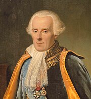
Although Gauss was the first to suggest the normal distribution law, Laplace made significant contributions.[note 4] It was Laplace who first posed the problem of aggregating several observations in 1774,[67] although his own solution led to the Laplacian distribution. It was Laplace who first calculated the value of the integral ∫ e−t2 dt = √π in 1782, providing the normalization constant for the normal distribution.[68] Finally, it was Laplace who in 1810 proved and presented to the Academy the fundamental central limit theorem, which emphasized the theoretical importance of the normal distribution.[69]
It is of interest to note that in 1809 an Irish-American mathematician Robert Adrain published two insightful but flawed derivations of the normal probability law, simultaneously and independently from Gauss.[70] His works remained largely unnoticed by the scientific community, until in 1871 they were exhumed by Abbe.[71]
In the middle of the 19th century Maxwell demonstrated that the normal distribution is not just a convenient mathematical tool, but may also occur in natural phenomena:[72] «The number of particles whose velocity, resolved in a certain direction, lies between x and x + dx is

Naming[edit]
Today, the concept is usually known in English as the normal distribution or Gaussian distribution. Other less common names include Gauss distribution, Laplace-Gauss distribution, the law of error, the law of facility of errors, Laplace’s second law, Gaussian law.
Gauss himself apparently coined the term with reference to the «normal equations» involved in its applications, with normal having its technical meaning of orthogonal rather than «usual».[73] However, by the end of the 19th century some authors[note 5] had started using the name normal distribution, where the word «normal» was used as an adjective – the term now being seen as a reflection of the fact that this distribution was seen as typical, common – and thus «normal». Peirce (one of those authors) once defined «normal» thus: «…the ‘normal’ is not the average (or any other kind of mean) of what actually occurs, but of what would, in the long run, occur under certain circumstances.»[74] Around the turn of the 20th century Pearson popularized the term normal as a designation for this distribution.[75]
Many years ago I called the Laplace–Gaussian curve the normal curve, which name, while it avoids an international question of priority, has the disadvantage of leading people to believe that all other distributions of frequency are in one sense or another ‘abnormal’.
Also, it was Pearson who first wrote the distribution in terms of the standard deviation σ as in modern notation. Soon after this, in year 1915, Fisher added the location parameter to the formula for normal distribution, expressing it in the way it is written nowadays:

The term «standard normal», which denotes the normal distribution with zero mean and unit variance came into general use around the 1950s, appearing in the popular textbooks by P. G. Hoel (1947) «Introduction to mathematical statistics» and A. M. Mood (1950) «Introduction to the theory of statistics«.[76]
See also[edit]
Notes[edit]
- ^ For example, this algorithm is given in the article Bc programming language.
- ^ De Moivre first published his findings in 1733, in a pamphlet «Approximatio ad Summam Terminorum Binomii (a + b)n in Seriem Expansi» that was designated for private circulation only. But it was not until the year 1738 that he made his results publicly available. The original pamphlet was reprinted several times, see for example Walker (1985).
- ^ «It has been customary certainly to regard as an axiom the hypothesis that if any quantity has been determined by several direct observations, made under the same circumstances and with equal care, the arithmetical mean of the observed values affords the most probable value, if not rigorously, yet very nearly at least, so that it is always most safe to adhere to it.» — Gauss (1809, section 177)
- ^ «My custom of terming the curve the Gauss–Laplacian or normal curve saves us from proportioning the merit of discovery between the two great astronomer mathematicians.» quote from Pearson (1905, p. 189)
- ^ Besides those specifically referenced here, such use is encountered in the works of Peirce, Galton (Galton (1889, chapter V)) and Lexis (Lexis (1878), Rohrbasser & Véron (2003)) c. 1875.[citation needed]
References[edit]
Citations[edit]
- ^ Norton, Matthew; Khokhlov, Valentyn; Uryasev, Stan (2019). «Calculating CVaR and bPOE for common probability distributions with application to portfolio optimization and density estimation» (PDF). Annals of Operations Research. Springer. 299 (1–2): 1281–1315. doi:10.1007/s10479-019-03373-1. Retrieved February 27, 2023.
- ^ Normal Distribution, Gale Encyclopedia of Psychology
- ^ Casella & Berger (2001, p. 102)
- ^ Lyon, A. (2014). Why are Normal Distributions Normal?, The British Journal for the Philosophy of Science.
- ^ a b «Normal Distribution». www.mathsisfun.com. Retrieved August 15, 2020.
- ^ Stigler (1982)
- ^ Halperin, Hartley & Hoel (1965, item 7)
- ^ McPherson (1990, p. 110)
- ^ Bernardo & Smith (2000, p. 121)
- ^ Scott, Clayton; Nowak, Robert (August 7, 2003). «The Q-function». Connexions.
- ^ Barak, Ohad (April 6, 2006). «Q Function and Error Function» (PDF). Tel Aviv University. Archived from the original (PDF) on March 25, 2009.
- ^ Weisstein, Eric W. «Normal Distribution Function». MathWorld.
- ^ Abramowitz, Milton; Stegun, Irene Ann, eds. (1983) [June 1964]. «Chapter 26, eqn 26.2.12». Handbook of Mathematical Functions with Formulas, Graphs, and Mathematical Tables. Applied Mathematics Series. Vol. 55 (Ninth reprint with additional corrections of tenth original printing with corrections (December 1972); first ed.). Washington D.C.; New York: United States Department of Commerce, National Bureau of Standards; Dover Publications. p. 932. ISBN 978-0-486-61272-0. LCCN 64-60036. MR 0167642. LCCN 65-12253.
- ^ Cover, Thomas M.; Thomas, Joy A. (2006). Elements of Information Theory. John Wiley and Sons. p. 254. ISBN 9780471748816.
- ^ Park, Sung Y.; Bera, Anil K. (2009). «Maximum Entropy Autoregressive Conditional Heteroskedasticity Model» (PDF). Journal of Econometrics. 150 (2): 219–230. CiteSeerX 10.1.1.511.9750. doi:10.1016/j.jeconom.2008.12.014. Archived from the original (PDF) on March 7, 2016. Retrieved June 2, 2011.
- ^ Geary RC(1936) The distribution of the «Student’s» ratio for the non-normal samples». Supplement to the Journal of the Royal Statistical Society 3 (2): 178–184
- ^ Lukacs, Eugene (March 1942). «A Characterization of the Normal Distribution». Annals of Mathematical Statistics. 13 (1): 91–93. doi:10.1214/AOMS/1177731647. ISSN 0003-4851. JSTOR 2236166. MR 0006626. Zbl 0060.28509. Wikidata Q55897617.
- ^ a b c Patel & Read (1996, [2.1.4])
- ^ Fan (1991, p. 1258)
- ^ Patel & Read (1996, [2.1.8])
- ^ Papoulis, Athanasios. Probability, Random Variables and Stochastic Processes (4th ed.). p. 148.
- ^ Bryc (1995, p. 23)
- ^ Bryc (1995, p. 24)
- ^ Cover & Thomas (2006, p. 254)
- ^ Williams, David (2001). Weighing the odds : a course in probability and statistics (Reprinted. ed.). Cambridge [u.a.]: Cambridge Univ. Press. pp. 197–199. ISBN 978-0-521-00618-7.
- ^ Smith, José M. Bernardo; Adrian F. M. (2000). Bayesian theory (Reprint ed.). Chichester [u.a.]: Wiley. pp. 209, 366. ISBN 978-0-471-49464-5.
- ^ O’Hagan, A. (1994) Kendall’s Advanced Theory of statistics, Vol 2B, Bayesian Inference, Edward Arnold. ISBN 0-340-52922-9 (Section 5.40)
- ^ a b Bryc (1995, p. 35)
- ^ UIUC, Lecture 21. The Multivariate Normal Distribution, 21.6:»Individually Gaussian Versus Jointly Gaussian».
- ^ Edward L. Melnick and Aaron Tenenbein, «Misspecifications of the Normal Distribution», The American Statistician, volume 36, number 4 November 1982, pages 372–373
- ^ «Kullback Leibler (KL) Distance of Two Normal (Gaussian) Probability Distributions». Allisons.org. December 5, 2007. Retrieved March 3, 2017.
- ^ Jordan, Michael I. (February 8, 2010). «Stat260: Bayesian Modeling and Inference: The Conjugate Prior for the Normal Distribution» (PDF).
- ^ Amari & Nagaoka (2000)
- ^ «Normal Approximation to Poisson Distribution». Stat.ucla.edu. Retrieved March 3, 2017.
- ^ a b Das, Abhranil (2020). «A method to integrate and classify normal distributions». arXiv:2012.14331 [stat.ML].
- ^ Bryc (1995, p. 27)
- ^ Weisstein, Eric W. «Normal Product Distribution». MathWorld. wolfram.com.
- ^ Lukacs, Eugene (1942). «A Characterization of the Normal Distribution». The Annals of Mathematical Statistics. 13 (1): 91–3. doi:10.1214/aoms/1177731647. ISSN 0003-4851. JSTOR 2236166.
- ^ Basu, D.; Laha, R. G. (1954). «On Some Characterizations of the Normal Distribution». Sankhyā. 13 (4): 359–62. ISSN 0036-4452. JSTOR 25048183.
- ^ Lehmann, E. L. (1997). Testing Statistical Hypotheses (2nd ed.). Springer. p. 199. ISBN 978-0-387-94919-2.
- ^ Patel & Read (1996, [2.3.6])
- ^ Galambos & Simonelli (2004, Theorem 3.5)
- ^ a b Lukacs & King (1954)
- ^ Quine, M.P. (1993). «On three characterisations of the normal distribution». Probability and Mathematical Statistics. 14 (2): 257–263.
- ^ John, S (1982). «The three parameter two-piece normal family of distributions and its fitting». Communications in Statistics — Theory and Methods. 11 (8): 879–885. doi:10.1080/03610928208828279.
- ^ a b Krishnamoorthy (2006, p. 127)
- ^ Krishnamoorthy (2006, p. 130)
- ^ Krishnamoorthy (2006, p. 133)
- ^ Huxley (1932)
- ^ Jaynes, Edwin T. (2003). Probability Theory: The Logic of Science. Cambridge University Press. pp. 592–593. ISBN 9780521592710.
- ^ Oosterbaan, Roland J. (1994). «Chapter 6: Frequency and Regression Analysis of Hydrologic Data» (PDF). In Ritzema, Henk P. (ed.). Drainage Principles and Applications, Publication 16 (second revised ed.). Wageningen, The Netherlands: International Institute for Land Reclamation and Improvement (ILRI). pp. 175–224. ISBN 978-90-70754-33-4.
- ^ Why Most Published Research Findings Are False, John P. A. Ioannidis, 2005
- ^ Wichura, Michael J. (1988). «Algorithm AS241: The Percentage Points of the Normal Distribution». Applied Statistics. 37 (3): 477–84. doi:10.2307/2347330. JSTOR 2347330.
- ^ Johnson, Kotz & Balakrishnan (1995, Equation (26.48))
- ^ Kinderman & Monahan (1977)
- ^ Leva (1992)
- ^ Marsaglia & Tsang (2000)
- ^ Karney (2016)
- ^ Monahan (1985, section 2)
- ^ Wallace (1996)
- ^ Johnson, Kotz & Balakrishnan (1994, p. 85)
- ^ Le Cam & Lo Yang (2000, p. 74)
- ^ De Moivre, Abraham (1733), Corollary I – see Walker (1985, p. 77)
- ^ Stigler (1986, p. 76)
- ^ Gauss (1809, section 177)
- ^ Gauss (1809, section 179)
- ^ Laplace (1774, Problem III)
- ^ Pearson (1905, p. 189)
- ^ Stigler (1986, p. 144)
- ^ Stigler (1978, p. 243)
- ^ Stigler (1978, p. 244)
- ^ Maxwell (1860, p. 23)
- ^ Jaynes, Edwin J.; Probability Theory: The Logic of Science, Ch. 7.
- ^ Peirce, Charles S. (c. 1909 MS), Collected Papers v. 6, paragraph 327.
- ^ Kruskal & Stigler (1997).
- ^ «Earliest uses… (entry STANDARD NORMAL CURVE)».
- ^ Sun, Jingchao; Kong, Maiying; Pal, Subhadip (June 22, 2021). «The Modified-Half-Normal distribution: Properties and an efficient sampling scheme». Communications in Statistics — Theory and Methods. 52 (5): 1591–1613. doi:10.1080/03610926.2021.1934700. ISSN 0361-0926. S2CID 237919587.
Sources[edit]
- Aldrich, John; Miller, Jeff. «Earliest Uses of Symbols in Probability and Statistics».
- Aldrich, John; Miller, Jeff. «Earliest Known Uses of Some of the Words of Mathematics». In particular, the entries for «bell-shaped and bell curve», «normal (distribution)», «Gaussian», and «Error, law of error, theory of errors, etc.».
- Amari, Shun-ichi; Nagaoka, Hiroshi (2000). Methods of Information Geometry. Oxford University Press. ISBN 978-0-8218-0531-2.
- Bernardo, José M.; Smith, Adrian F. M. (2000). Bayesian Theory. Wiley. ISBN 978-0-471-49464-5.
- Bryc, Wlodzimierz (1995). The Normal Distribution: Characterizations with Applications. Springer-Verlag. ISBN 978-0-387-97990-8.
- Casella, George; Berger, Roger L. (2001). Statistical Inference (2nd ed.). Duxbury. ISBN 978-0-534-24312-8.
- Cody, William J. (1969). «Rational Chebyshev Approximations for the Error Function». Mathematics of Computation. 23 (107): 631–638. doi:10.1090/S0025-5718-1969-0247736-4.
- Cover, Thomas M.; Thomas, Joy A. (2006). Elements of Information Theory. John Wiley and Sons.
- de Moivre, Abraham (1738). The Doctrine of Chances. ISBN 978-0-8218-2103-9.
- Fan, Jianqing (1991). «On the optimal rates of convergence for nonparametric deconvolution problems». The Annals of Statistics. 19 (3): 1257–1272. doi:10.1214/aos/1176348248. JSTOR 2241949.
- Galton, Francis (1889). Natural Inheritance (PDF). London, UK: Richard Clay and Sons.
- Galambos, Janos; Simonelli, Italo (2004). Products of Random Variables: Applications to Problems of Physics and to Arithmetical Functions. Marcel Dekker, Inc. ISBN 978-0-8247-5402-0.
- Gauss, Carolo Friderico (1809). Theoria motvs corporvm coelestivm in sectionibvs conicis Solem ambientivm [Theory of the Motion of the Heavenly Bodies Moving about the Sun in Conic Sections] (in Latin). Hambvrgi, Svmtibvs F. Perthes et I. H. Besser. English translation.
- Gould, Stephen Jay (1981). The Mismeasure of Man (first ed.). W. W. Norton. ISBN 978-0-393-01489-1.
- Halperin, Max; Hartley, Herman O.; Hoel, Paul G. (1965). «Recommended Standards for Statistical Symbols and Notation. COPSS Committee on Symbols and Notation». The American Statistician. 19 (3): 12–14. doi:10.2307/2681417. JSTOR 2681417.
- Hart, John F.; et al. (1968). Computer Approximations. New York, NY: John Wiley & Sons, Inc. ISBN 978-0-88275-642-4.
- «Normal Distribution», Encyclopedia of Mathematics, EMS Press, 2001 [1994]
- Herrnstein, Richard J.; Murray, Charles (1994). The Bell Curve: Intelligence and Class Structure in American Life. Free Press. ISBN 978-0-02-914673-6.
- Huxley, Julian S. (1932). Problems of Relative Growth. London. ISBN 978-0-486-61114-3. OCLC 476909537.
- Johnson, Norman L.; Kotz, Samuel; Balakrishnan, Narayanaswamy (1994). Continuous Univariate Distributions, Volume 1. Wiley. ISBN 978-0-471-58495-7.
- Johnson, Norman L.; Kotz, Samuel; Balakrishnan, Narayanaswamy (1995). Continuous Univariate Distributions, Volume 2. Wiley. ISBN 978-0-471-58494-0.
- Karney, C. F. F. (2016). «Sampling exactly from the normal distribution». ACM Transactions on Mathematical Software. 42 (1): 3:1–14. arXiv:1303.6257. doi:10.1145/2710016. S2CID 14252035.
- Kinderman, Albert J.; Monahan, John F. (1977). «Computer Generation of Random Variables Using the Ratio of Uniform Deviates». ACM Transactions on Mathematical Software. 3 (3): 257–260. doi:10.1145/355744.355750. S2CID 12884505.
- Krishnamoorthy, Kalimuthu (2006). Handbook of Statistical Distributions with Applications. Chapman & Hall/CRC. ISBN 978-1-58488-635-8.
- Kruskal, William H.; Stigler, Stephen M. (1997). Spencer, Bruce D. (ed.). Normative Terminology: ‘Normal’ in Statistics and Elsewhere. Statistics and Public Policy. Oxford University Press. ISBN 978-0-19-852341-3.
- Laplace, Pierre-Simon de (1774). «Mémoire sur la probabilité des causes par les événements». Mémoires de l’Académie Royale des Sciences de Paris (Savants étrangers), Tome 6: 621–656. Translated by Stephen M. Stigler in Statistical Science 1 (3), 1986: JSTOR 2245476.
- Laplace, Pierre-Simon (1812). Théorie analytique des probabilités [Analytical theory of probabilities]. Paris, Ve. Courcier.
- Le Cam, Lucien; Lo Yang, Grace (2000). Asymptotics in Statistics: Some Basic Concepts (second ed.). Springer. ISBN 978-0-387-95036-5.
- Leva, Joseph L. (1992). «A fast normal random number generator» (PDF). ACM Transactions on Mathematical Software. 18 (4): 449–453. CiteSeerX 10.1.1.544.5806. doi:10.1145/138351.138364. S2CID 15802663. Archived from the original (PDF) on July 16, 2010.
- Lexis, Wilhelm (1878). «Sur la durée normale de la vie humaine et sur la théorie de la stabilité des rapports statistiques». Annales de Démographie Internationale. Paris. II: 447–462.
- Lukacs, Eugene; King, Edgar P. (1954). «A Property of Normal Distribution». The Annals of Mathematical Statistics. 25 (2): 389–394. doi:10.1214/aoms/1177728796. JSTOR 2236741.
- McPherson, Glen (1990). Statistics in Scientific Investigation: Its Basis, Application and Interpretation. Springer-Verlag. ISBN 978-0-387-97137-7.
- Marsaglia, George; Tsang, Wai Wan (2000). «The Ziggurat Method for Generating Random Variables». Journal of Statistical Software. 5 (8). doi:10.18637/jss.v005.i08.
- Marsaglia, George (2004). «Evaluating the Normal Distribution». Journal of Statistical Software. 11 (4). doi:10.18637/jss.v011.i04.
- Maxwell, James Clerk (1860). «V. Illustrations of the dynamical theory of gases. — Part I: On the motions and collisions of perfectly elastic spheres». Philosophical Magazine. Series 4. 19 (124): 19–32. doi:10.1080/14786446008642818.
- Monahan, J. F. (1985). «Accuracy in random number generation». Mathematics of Computation. 45 (172): 559–568. doi:10.1090/S0025-5718-1985-0804945-X.
- Patel, Jagdish K.; Read, Campbell B. (1996). Handbook of the Normal Distribution (2nd ed.). CRC Press. ISBN 978-0-8247-9342-5.
- Pearson, Karl (1901). «On Lines and Planes of Closest Fit to Systems of Points in Space» (PDF). Philosophical Magazine. 6. 2 (11): 559–572. doi:10.1080/14786440109462720.
- Pearson, Karl (1905). «‘Das Fehlergesetz und seine Verallgemeinerungen durch Fechner und Pearson’. A rejoinder». Biometrika. 4 (1): 169–212. doi:10.2307/2331536. JSTOR 2331536.
- Pearson, Karl (1920). «Notes on the History of Correlation». Biometrika. 13 (1): 25–45. doi:10.1093/biomet/13.1.25. JSTOR 2331722.
- Rohrbasser, Jean-Marc; Véron, Jacques (2003). «Wilhelm Lexis: The Normal Length of Life as an Expression of the «Nature of Things»«. Population. 58 (3): 303–322. doi:10.3917/pope.303.0303.
- Shore, H (1982). «Simple Approximations for the Inverse Cumulative Function, the Density Function and the Loss Integral of the Normal Distribution». Journal of the Royal Statistical Society. Series C (Applied Statistics). 31 (2): 108–114. doi:10.2307/2347972. JSTOR 2347972.
- Shore, H (2005). «Accurate RMM-Based Approximations for the CDF of the Normal Distribution». Communications in Statistics – Theory and Methods. 34 (3): 507–513. doi:10.1081/sta-200052102. S2CID 122148043.
- Shore, H (2011). «Response Modeling Methodology». WIREs Comput Stat. 3 (4): 357–372. doi:10.1002/wics.151. S2CID 62021374.
- Shore, H (2012). «Estimating Response Modeling Methodology Models». WIREs Comput Stat. 4 (3): 323–333. doi:10.1002/wics.1199. S2CID 122366147.
- Stigler, Stephen M. (1978). «Mathematical Statistics in the Early States». The Annals of Statistics. 6 (2): 239–265. doi:10.1214/aos/1176344123. JSTOR 2958876.
- Stigler, Stephen M. (1982). «A Modest Proposal: A New Standard for the Normal». The American Statistician. 36 (2): 137–138. doi:10.2307/2684031. JSTOR 2684031.
- Stigler, Stephen M. (1986). The History of Statistics: The Measurement of Uncertainty before 1900. Harvard University Press. ISBN 978-0-674-40340-6.
- Stigler, Stephen M. (1999). Statistics on the Table. Harvard University Press. ISBN 978-0-674-83601-3.
- Walker, Helen M. (1985). «De Moivre on the Law of Normal Probability» (PDF). In Smith, David Eugene (ed.). A Source Book in Mathematics. Dover. ISBN 978-0-486-64690-9.
- Wallace, C. S. (1996). «Fast pseudo-random generators for normal and exponential variates». ACM Transactions on Mathematical Software. 22 (1): 119–127. doi:10.1145/225545.225554. S2CID 18514848.
- Weisstein, Eric W. «Normal Distribution». MathWorld.
- West, Graeme (2009). «Better Approximations to Cumulative Normal Functions» (PDF). Wilmott Magazine: 70–76.
- Zelen, Marvin; Severo, Norman C. (1964). Probability Functions (chapter 26). Handbook of mathematical functions with formulas, graphs, and mathematical tables, by Abramowitz, M.; and Stegun, I. A.: National Bureau of Standards. New York, NY: Dover. ISBN 978-0-486-61272-0.
External links[edit]
- «Normal distribution», Encyclopedia of Mathematics, EMS Press, 2001 [1994]
- Normal distribution calculator