Распределение пуассона как найти вероятность - Исправление недочетов и поиск решений вместе с Examum.ru

Определение распределения Пуассона

Распределение Пуассона относится к процессу определения вероятности повторения событий в течение определенного периода времени. Переменные для этого распределения вероятностей должны быть счетными, случайными и независимыми.

Этот статистический инструмент используется для понимания будущих возможностей и тенденций. Он используется бизнес-организациями, финансовыми аналитиками. Финансовые аналитики. Финансовый аналитик анализирует проект или компанию с основной целью консультировать руководство / клиентов по поводу жизнеспособных инвестиционных решений. Они проводят тщательный финансовый анализ и делают подходящие объективные прогнозы, чтобы прийти к своим выводам. Читать далее, исследователи рынка, астрономы, ученые, физиологи, спортивные власти и правительственные учреждения. Впервые он был введен Симеоном Дени Пуассоном в 1830 году. Используя этот метод, французский математик рассчитал вероятность успеха в азартных играх.

Оглавление

Определение распределения Пуассона
- Как работает распределение Пуассона?
- Формула распределения Пуассона
- Расчет с графиком
- Примеры распределения Пуассона в Excel
  - Пример №1
  - Пример #2
- Приложения распределения Пуассона
- Часто задаваемые вопросы (FAQ)
- Рекомендуемые статьи

Распределение Пуассона — это однопараметрический вероятностный инструмент, используемый для определения шансов на успех, т. е. для определения того, сколько раз событие происходит в течение определенного периода времени.
Формула распределения Пуассона: P(x;µ)=(e^(-µ) µ^x)/x!.
Распределение считается моделью Пуассона, когда количество вхождений является счетным (в целых числах), случайным и независимым. Другими словами, оно должно быть независимым от других событий и их возникновения.
Кроме того, среднее значение X ∼P(µ) = µ; Дисперсия X ∼P(µ) = µ; и стандартное отклонение X ∼P(µ) = +√µ.

Как работает распределение Пуассона?

Распределение Пуассона есть не что иное, как прогноз события, происходящего в определенный период. Устанавливается возможность возникновения события заданное количество раз для заданного периода времени. Например, шансы получить определенное количество ударов сердца в течение минуты — это распределение вероятностей. Рассмотрим другой пример, предположим, что больница хочет реструктурировать персонал своего отделения неотложной помощи. Скажем, больница ежедневно принимает три неотложных случая. Администрация использует распределение Пуассона, чтобы определить возможность приема пяти экстренных случаев в день для найма резервного персонала.

Этот статистический инструмент является однопараметрическим. В результате знание средней переменной возникновения события можно использовать для определения других возможностей. Распределение ПуассонаРаспределение ПуассонаРаспределение Пуассона относится к процессу определения вероятности повторения событий в течение определенного периода времени. X ∼ P(μ). Более того, мы также можем найти его среднее значение, дисперсию и стандартное отклонение, используя следующие уравнения:

Среднее значение X ∼P(µ) = µ
Дисперсия X ∼P(µ) = µ
Стандартное отклонениеСтандартное отклонениеСтандартное отклонение (SD) — это популярный статистический инструмент, обозначаемый греческой буквой «σ», для измерения вариации или дисперсии набора значений данных относительно их среднего (среднего) значения, таким образом интерпретируя надежность данных.Подробнее о X ∼P(μ) = +√μ

Результаты двух распределений Пуассона можно суммировать, чтобы получить вероятность более широкой случайной величины. То есть X1∼P(µ1) и X2∼P(µ2) могут предоставить значение третьей переменной Y. Здесь Y = X1+X2∼P (µ1+ µ2). Например, предположим, что хоккейная команда выигрывает в среднем два матча на каждые пять сыгранных игр. Какова вероятность выиграть одно соревнование в этом году? Команда может выиграть 0 или 1 матч. Таким образом, чтобы вычислить желаемые результаты, сложите обе вероятности. То есть сложите вероятность выигрыша нулевого матча и вероятность выигрыша одного матча.

В 1830 году Симеон Дени Пуассон представил модель распределения Пуассона. Он был французским математиком, который вычислил шансы на успех в азартных играх, используя этот метод. Однако это был непопулярный инструмент среди игроков. Тем не менее, концепция приобрела значение в области статистики после Второй мировой войны. Британский статистик Р. Д. Кларк использовал этот инструмент, чтобы помочь британскому правительству получить представление о немецких бомбардировках Лондона. Кларк проанализировал, что немцы сбросили бомбы случайным образом. Кларк пришел к выводу, что в атаках не указан регион или город.

Формула распределения Пуассона

Это распределение вероятности определяет вероятность повторения события в течение заданного интервала времени. Формула выглядит следующим образом:

Здесь P(x; µ) — вероятность того, что событие произойдет определенное число раз за определенный период;

e обозначает число Эйлера, основное значение которого равно 2,72;

µ — среднее количество вхождений за определенный период; и

Икс! является факториалом числа событий, для которых определяется вероятность.

Расчет с графиком

Рассмотрим следующее числовое значение, чтобы лучше понять вычисления, используемые в этом математическом инструменте.

Компания-производитель часов хочет сократить количество бракованных изделий. Было отобрано в среднем 100 партий, и было обнаружено, что 7 часов из каждой партии были бракованными. Какова вероятность того, что 10 часов будут бракованными в одной партии?

Решение:

Данный:

Среднее количество бракованных часов в партии (µ) = 7

Ожидаемое количество бракованных часов в конкретной партии (x) = 10

Р (х; мк) = [e^(-μ) μ^x]/Икс!

Р (10;7) = [e^ (-7) 7^10]/10!

Р (10;7) = 0,07098 или 7,098%

Таким образом, вероятность того, что в данной партии будет 10 бракованных часов, составляет 7,098%.

График распределения Пуассона

На том же примере изобразим на графике вероятность наличия 0,1, 2, 3, 4, 5, 6, 7, 8, 9, 10, 11, 12, 13, 14 бракованных часов.

Примеры распределения Пуассона в Excel

Рассмотрим этот простой пример Excel, чтобы лучше понять, как применяется формула распределения Пуассона.

Пример №1

Среднее количество событий в заданном временном интервале равно 10. Какова вероятность того, что это событие произойдет 15 раз?

В этом примере u = среднее количество появлений события = 10

И х = 15

Следовательно, расчет распределения Пуассона можно выполнить следующим образом:

P (15;10) = e^(-10)*10^15/15!

Р (15; 10) = 0,0347 = 3,47%

Следовательно, вероятность того, что это событие произойдет 15 раз, составляет 3,47%.

Пример #2

Другое использование формулы Пуассона в страховой отрасли. Компания, занимающаяся страховым бизнесом, определяет размер страховой премии на основе количества исков и суммы требований в год. Так, для оценки суммы своей премии страховая компания будет определять среднее количество заявленной суммы в год. Затем, основываясь на этом среднем, он также определит минимальное и максимальное количество исков, которые можно обоснованно подать в год. Основываясь на максимальном количестве суммы претензии, а также стоимости и прибыли от премии, страховая компания определит, какая сумма премии будет хорошей для безубыточности.

Скажем, среднее количество претензий, обрабатываемых страховой компанией в день, равно 5. Она выяснит, какова вероятность 10 претензий в день.

Следовательно, расчет можно провести следующим образом:

Р(10;5) = е^(-5). 5^10/10!

Р(10;5) = 1,81%

Следовательно, вероятность того, что компания будет иметь 10 претензий в день, очень мала. На основании этих данных компания может принять решение о размере премии.

Приложения распределения Пуассона

Распределение Пуассона полезно для прогнозирования, отслеживания и повышения эффективности компании. Он часто применяется для оценки эффективности бизнеса и направления организационных усилий для достижения операционной эффективности. Например, руководство может определить пиковые часы продаж и эффективности обслуживания клиентов, чтобы спланировать потребности в рабочей силе. Таким образом, можно комфортно переносить периоды спешки и суеты.

Этот статистический инструмент очень эффективен для проверки осуществимости и жизнеспособности страхового покрытия. Он включает в себя анализ различных факторов, таких как вероятность несчастных случаев, стоимость страхового покрытия, количество раз, когда может быть предъявлен иск, является ли компания чрезмерно застрахованной или недостаточно застрахованной. Кроме того, используя этот метод, менеджеры по производству контролируют потери, отслеживая количество бракованных изделий в каждом цикле производства.

Это одинаково важный инструмент в области финансов для фондовых аналитиков и рыночных прогнозов. Это помогает определить уровень риска, связанный с инвестициями в ценные бумаги. Это достигается путем установления возможности падения рынка в определенный период. Этот метод даже облегчает анализ поведения инвесторов и частоты инвестиций.

Часто задаваемые вопросы (FAQ)

Что такое распределение Пуассона в статистике?

Распределение Пуассона — это не что иное, как предсказание события, происходящего в течение заданного периода времени. Устанавливается возможность возникновения события заданное количество раз для заданного периода времени.

Какими свойствами обладает распределение Пуассона?

Модель называется распределением Пуассона, если она обладает следующими свойствами:

• Возможность успеха в конкретный период времени не зависит от его более раннего наступления.
• Переменные или количество вхождений должны быть целыми числами, т. е. быть исчисляемыми.
• Шансы на успешный исход более одного раза за данный период ничтожны.
• Следует указать значение µ, т. е. среднее количество событий за определенный период.

В чем разница между процессом Пуассона и распределением Пуассона?

Процесс Пуассона — это непрерывное возникновение независимых событий, подобных безостановочному сердцебиению человека. В то время как распределение Пуассона — это средство нахождения возможности повторения события несколько раз за определенный период, т. е. количества повторений события в процессе Пуассона. Например, шансы получить определенное количество ударов сердца в течение минуты — это распределение вероятностей.

Закон распределения Пуассона

На этой странице мы собрали примеры решения учебных задач, где используется распределение Пуассона.

Краткая теория

Рассмотрим некоторый поток событий, в котором события наступают независимо друг от друга и с некоторой фиксированной средней интенсивностью $lambda$ (событий в единицу времени). Тогда случайная величина $X$, равная числу событий $k$, произошедших за фиксированное время, имеет распределение Пуассона. Вероятности вычисляются по следующей формуле:

$$
P(X=k)=frac{lambda^k}{k!}cdot e^{-lambda}, k=0,1,2,…
$$

Для пуассоновской случайной величины математическое ожидание и дисперсия совпадают с интенсивностью потока событий:

$$M(X)=lambda, quad D(X)=lambda.$$

Распределение Пуассона играет важную роль в теории массового обслуживания. При увеличении $lambda$ данное распределение стремится к нормальному распределению $N(lambda, sqrt{lambda})$. В свою очередь, оно само является «приближенной» моделью биномиального распределения при больших $n$ и крайне малых $p$ (см. теорию про формулу Пуассона).

Понравилось? Добавьте в закладки

Примеры решенных задач

Задача 1. Среднее число самолетов, взлетающих с полевого аэродрома за одни сутки, равно 10. Найти вероятность того, что за 6 часов взлетят:
А) три самолета,
Б) не менее двух самолетов.

Задача 2. На автовокзале время прибытия автобусов различных рейсов объявляет дежурный. Появление информации о различных рейсах происходит случайной и независимо друг от друга. В среднем на автовокзал прибывает 5 рейсов каждые полчаса.
А) Составьте ряд распределения числа сообщений о прибытии автобусов в течение получаса.
Б) Найдите числовые характеристики этого распределения.
В) Запишите функцию распределения вероятностей и постройте ее график.
Г) Чему равна вероятность того, что в течение получаса прибудут не менее трех автобусов?
Д) Чему равна вероятность того, что в течение четверти часа не прибудет ни один автобус?

Задача 3. АТС получает в среднем за час 480 вызовов. Определить вероятность того, что за данную минуту она получит: ровно 3 вызова; от 2 до 5 вызовов.

Задача 4. Случайная величина $X$ распределена по закону Пуассона с параметром $lambda=0,8$. Необходимо:
А) выписать формулу для вычисления вероятности $P(X=m)$;
Б) найти вероятность $P(1 le X lt 3)$;
В) найти математическое ожидание $M(2X+5)$ и дисперсию $D(5-2X)$.

Задача 5. Среднее число ошибочных соединений, приходящееся на одного телефонного абонента в единицу времени, равно 8. Какова вероятность того, что для данного абонента число ошибочных соединений будет больше 4?

Задача 6. В среднем в магазин заходят 3 человека в минуту. Найти вероятность того, что за 2 минуты в магазин зайдет не более 1 человека.

Задача 7. Автомобиль проходит технический осмотр и обслуживание. Число неисправностей, обнаруженных во время техосмотра, распределяется по закону Пуассона с параметром 0,63. Если неисправностей не обнаружено, техническое обслуживание автомобиля продолжается в среднем 2 ч. Если обнаружены одна или две неисправности, то на устранение каждой из них тратится в среднем еще полчаса. Если обнаружено больше двух неисправностей, то автомобиль становится на профилактический ремонт, где он находится в среднем 4 ч.
Определите закон распределения среднего времени $T$ обслуживания и ремонта автомобиля и его математическое ожидание $M(T)$.

Задача 8. В тексте учебника по психологии содержатся опечатки: в среднем, одна на
десять страниц. Пусть Х – число опечаток на одной странице. Определить закон распределения для Х. Найти вероятность, что на странице есть хотя бы одна опечатка.

Мы отлично умеем решать задачи по теории вероятностей

Решебник по терверу

Если решения нужны срочно и почти даром? Ищите в решебнике по теории вероятностей:

Источник

Распределение Пуассона — одно из самых популярных распределений в статистике.

Чтобы понять распределение Пуассона, сначала нужно понять эксперименты Пуассона.

Пуассоновые эксперименты

Эксперимент Пуассона — это эксперимент, обладающий следующими свойствами:

Количество успехов в эксперименте можно подсчитать.
Известно среднее количество успехов, которое происходит в течение определенного интервала времени (или пространства).
Каждый результат является независимым.
Вероятность того, что произойдет успех, пропорциональна размеру интервала.

Одним из примеров эксперимента Пуассона является количество рождений в час в данной больнице. Например, предположим, что в конкретной больнице происходит в среднем 10 родов в час. Это эксперимент Пуассона, поскольку он обладает следующими четырьмя свойствами:

Количество успехов в эксперименте можно подсчитать – Мы можем подсчитать количество рождений.
Известно среднее количество успехов, которое происходит в течение определенного интервала времени. Известно, что в среднем происходит 10 рождений в час.
Каждый результат независим — вероятность того, что одна мать родит в течение данного часа, не зависит от вероятности того, что другая мать родит.
Вероятность того, что произойдет успех, пропорциональна размеру интервала: чем длиннее интервал времени, тем выше вероятность того, что произойдет рождение.

Мы можем использовать распределение Пуассона, чтобы ответить на вопросы о вероятностях этого эксперимента Пуассона, такие как:

Какова вероятность того, что в данный час произойдет более 12 родов?
Какова вероятность того, что в данный час произойдет менее 5 родов?
Какова вероятность того, что в данный час произойдет от 8 до 11 родов?

Распределение Пуассона

Распределение Пуассона описывает вероятность получения k успехов за заданный интервал времени.

Если случайная величина X подчиняется распределению Пуассона, то вероятность того, что X = k успехов, можно найти по следующей формуле:

P(X=k) = λk * e – λ / k !

куда:

λ: среднее количество успехов за определенный интервал
k: количество успехов
e: константа, равная приблизительно 2,71828.

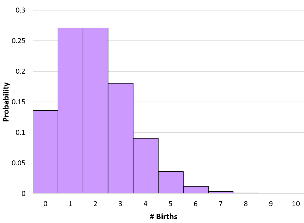
Например, предположим, что в конкретной больнице в среднем рождается 2 человека в час. Мы можем использовать приведенную выше формулу, чтобы определить вероятность рождения 0, 1, 2, 3 и т. д. в данный час:

P(X=0) = 2 0 * e – 2 / 0! = 0,1353

P(X=1) = 2 1 * e – 2 / 1! = 0,2707

P(X=2) = 2 2 * e – 2 / 2! = 0,2707

P(X=3) = 2 3 * e – 2 / 3! = 0,1805

Мы можем рассчитать вероятность для любого числа рождений вплоть до бесконечности. Мы создаем, а затем создаем простую гистограмму для визуализации этого распределения вероятностей:

Вычисление кумулятивных вероятностей Пуассона

Несложно рассчитать одну вероятность Пуассона (например, вероятность того, что в больнице произойдет 3 рождения в течение заданного часа), используя приведенную выше формулу, но для расчета кумулятивной вероятности Пуассона нам нужно добавить индивидуальные вероятности.

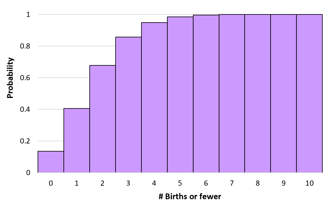
Например, предположим, что мы хотим узнать вероятность того, что в больнице будет 1 или меньше родов в данный час. Мы будем использовать следующую формулу для расчета этой вероятности:

P(X≤1) = P(X=0) + P(X=1) = 0,1353 + 0,2707 = 0,406

Это известно как кумулятивная вероятность , потому что она включает в себя добавление более одной вероятности. Мы можем рассчитать кумулятивную вероятность появления k или меньше рождений в данный час, используя аналогичную формулу:

Р(Х≤0) = Р(Х=0) = 0,1353

P(X≤1) = P(X=0) + P(X=1) = 0,1353 + 0,2707 = 0,406

P(X≤2) = P(X=0) + P(X=1) + P(X=2) = 0,1353 + 0,2707 + 0,2707 = 0,6767

Мы можем рассчитать эти кумулятивные вероятности для любого числа рождений вплоть до бесконечности. Затем мы можем создать гистограмму для визуализации этого кумулятивного распределения вероятностей:

Свойства распределения Пуассона

Распределение Пуассона обладает следующими свойствами:

Среднее значение распределения равно λ .

Дисперсия распределения также равна λ .

Стандартное отклонение распределения равно √ λ .

Например, предположим, что в больнице в среднем рождается 2 ребенка в час.

Среднее число рождений, которое мы ожидаем в данный час, составляет λ = 2 рождения.

Ожидаемая дисперсия числа рождений составляет λ = 2 рождения.

Проблемы практики распределения Пуассона

Используйте следующие практические задачи, чтобы проверить свои знания о распределении Пуассона.

Примечание. Мы будем использоватькалькулятор распределения Пуассона для расчета ответов на эти вопросы.

Проблема 1

Вопрос: Известно, что некий сайт делает 10 продаж в час. Какова вероятность того, что за данный час сайт совершит ровно 8 продаж?

Ответ: Используя калькулятор распределения Пуассона с λ = 10 и x = 8, мы находим, что P(X=8) = 0,1126 .

Проблема 2

Вопрос: Известно, что некий риелтор делает в среднем 5 продаж в месяц. Какова вероятность того, что в данном месяце она совершит более 7 продаж?

Ответ: Используя калькулятор распределения Пуассона с λ = 5 и x = 7, мы находим, что P(X>7) = 0,13337 .

Проблема 3

Вопрос: Известно, что в одной больнице рождается 4 человека в час. Какова вероятность того, что в данный час произойдет 4 или менее родов?

Ответ: Используя калькулятор распределения Пуассона с λ = 4 и x = 4, мы находим, что P(X≤4) = 0,62884 .

Дополнительные ресурсы

В следующих статьях объясняется, как работать с распределением Пуассона в различных статистических программах:

Как использовать распределение Пуассона в R
Как использовать распределение Пуассона в Excel
Как рассчитать вероятности Пуассона на калькуляторе TI-84
Реальные примеры распределения Пуассона
Калькулятор распределения Пуассона

Источник

Закон распределения Пуассона

Краткая теория
Примеры решения задач
Задачи контрольных и самостоятельных работ

Краткая теория

Дискретная случайная величина
имеет закон распределения Пуассона с
параметром

,
если она принимает значения 0,1,2,…,k,… (бесконечное, но счетное множество значений) с вероятностями

Ряд распределения закона Пуассона имеет вид:

Математическое ожидание и дисперсия случайной величины,
распределенной по закону Пуассона, совпадают и равны параметру этого закона,
т.е.

По закону Пуассона распределены, например, число рождений тройни,
число сбоев на автоматической линии, число отказов сложной системы в нормальном
режиме, число требований на обслуживания, поступивших в единицу времени в
системах массового обслуживания и тому подобное.

Если СВ представляет собой сумму двух независимых СВ,
распределенных каждая по закону Пуассона, то она также распределена по закону
Пуассона.

Распределение Пуассона также называют законом «редких» событий, так как оно всегда проявляется там, где производится большое
число испытаний, в каждом из которых с малой вероятностью происходит «редкое» событие.

Смежные темы решебника:

Биномиальный закон распределения дискретной случайной величины
Геометрический закон распределения дискретной случайной величины
Гипергеометрический закон распределения дискретной случайной величины
Простейший поток событий

Примеры решения задач

Пример 1

На
предприятии 1000 единиц оборудования определенного вида. Вероятность отказа
единицы оборудования в течение часа составляет 0,001. Составить закон
распределения числа отказов оборудования в течение часа. Найти числовые
характеристики.

Решение

На сайте можно заказать решение контрольной или самостоятельной работы, домашнего задания, отдельных задач. Для этого вам нужно только связаться со мной:

ВКонтакте
WhatsApp
Telegram

Мгновенная связь в любое время и на любом этапе заказа. Общение без посредников. Удобная и быстрая оплата переводом на карту СберБанка. Опыт работы более 25 лет.

Подробное решение в электронном виде (docx, pdf) получите точно в срок или раньше.

Случайная
величина

– число отказов оборудования, может принимать
значения

Воспользуемся
законом Пуассона:

где

Найдем
эти вероятности:

Найдем
вероятность того, что откажет более 5 единиц оборудования:

Искомый
закон распределения числа отказов оборудования в течение часа:

Проверка гипотезы о распределении выборки по закону Пуассона.

Математическое
ожидание и дисперсия случайной величины, распределенной по закону Пуассона
равна параметру

этого распределения:

Среднее
квадратическое отклонение:

Пример 2

Станок-автомат штампует детали. Вероятность того, что изготовленная
деталь окажется бракованной, равна 0,001 Найти вероятность того, что среди 350
деталей окажется ровно 3 бракованных.
Определить закон распределения СВ X и её числовые характеристики.

Решение

Вероятность
события, состоящее в том, что деталь окажется бракованной мало, а число

велико. Поэтому воспользуемся распределением
Пуассона:

Искомая
вероятность:

Закон
распределения СВ

Математическое
ожидание:

Дисперсия:

Среднее
квадратическое отклонение:

Пример 3

Найти среднее число бракованных изделий в партии изделий, если
вероятность того, что в этой партии содержится хотя бы одно бракованное
изделие, равна 0,92. Предполагается, что число бракованных изделий в
рассматриваемой партии распределено по закону Пуассона.

Решение

ВКонтакте
WhatsApp
Telegram

Подробное решение в электронном виде (docx, pdf) получите точно в срок или раньше.

Распределение
Пуассона:

Среднее
число бракованных изделий:

Пусть
событие

–в партии содержится хотя бы одно бракованное
изделие

Тогда
противоположное событие

– в партии нет ни одного бракованного изделия

Решая
уравнение, получаем:

Ответ:

Пример 4

Случайная величина ξ распределена по закону
Пуассона с параметром λ=0,2. Найти:

а)

;

б)

;

в)

Решение

Закон Пуассона:

Для закона Пуассона математическое ожидание:

Дисперсия:

а)

б)

в)

Ответ: а)

; б)

; в)

Пример 5

Случайные величины

распределены по закону Пуассона с одинаковым
математическим ожиданием, равным 6. Найдите математическое ожидание

Решение

ВКонтакте
WhatsApp
Telegram

Подробное решение в электронном виде (docx, pdf) получите точно в срок или раньше.

Поскольку случайные величины распределены по закону Пуассона и известны
их математические ожидания, соответствующие дисперсии равны:

Искомая величина:

Ответ: 504

Задачи контрольных и самостоятельных работ

Задача 1

Для пуассоновой случайной величины X
имеем

Найдите M(X)

Задача 2

Случайные величины X,Y распределены
по закону Пуассона. Найдите

, если M(X)=40 и M(Y)=70, а коэффициент корреляции X и
Y равен 0,8.

Задача 3

В
некоторой системе 810 приборов. Вероятность отказа каждого прибора в течение
заданного промежутка времени 0.001. Найти вероятность отказа не менее 3
приборов за данный промежуток времени. Найти характеристики данного
распределения случайной величины.

Задача 4

В партии
из 1000 изделий имеются 10 дефектных. Найти вероятность того, что среди 50
изделий, взятых наудачу из этой партии, ровно три окажутся дефектными.

Задача 5

Радиостанция
ведет передачу информации в течение 10 мкс. Работа ее происходит при наличии
хаотической импульсной помехи, среднее число импульсов которой в секунду
составляет

. Для срыва передачи
достаточно попадания одного импульса помехи в период работы станции. Считая,
что число импульсов помехи, попадающих в данный интервал времени, распределено
по закону Пуассона, найти вероятность срыва передачи информации.

Задача 6

Среди
семян пшеницы 0,6% семян сорняков. Какова вероятность при случайном отборе 1000
семян обнаружить не менее трех семян сорняков?

ВКонтакте
WhatsApp
Telegram

Подробное решение в электронном виде (docx, pdf) получите точно в срок или раньше.

Задача 7

На
телефонную станцию поступает в среднем 5 заявок на переговоры в минуту. Поток заявок
описывается распределением Пуассона. Рассчитать вероятность того, что за минуту
на станцию придут ровно две заявки.

Задача 8

Вероятность попадания в
цель при каждом выстреле равна 0,001. Найти вероятность попадания в цель ровно
100 раз, если было произведено 2000 выстрелов.

Задача 9

Вероятность
изготовления нестандартной детали p=0.003. Найти
вероятность того, что среди 1000 деталей окажется 4 нестандартных.

Задача 10

Вероятность
сбоя в работе банкомата при каждом запросе равна 0,0016. Банкомат обслуживает
2000 клиентов в неделю. Определить вероятность того, что при этом число сбоев
не превзойдет 3.

Задача 11

Прядильщица
обслуживает 800 веретен. Вероятность обрыва нити на одном веретене в течение
одной минуты 0,003. Найти вероятность того, что в течение одной минуты обрыв
произойдет на трех веретенах.

Задача 12

Телефонный кабель состоит из 400 жил. С какой вероятностью этим
кабелем можно подключить к телефонной сети не менее 395 абонентов, если для
подключения каждого из них нужна одна жила, а вероятность того, что она
повреждена – 0,0125.

Задача 13

Вероятность «сбоя» в работе телефонной станции при каждом вызове
равна 0.05. Поступило 100 вызовов. Определить вероятность того, что произойдет
не более 3 сбоев.

Задача 14

На базе получено 10000 электроламп. Вероятность того, что в пути
лампа разобьется, равна 0,0003. Найдите вероятность того, что среди полученных
ламп будет пять ламп разбито.

Задача 15

Завод отправил в торговую сеть 500 изделий. Вероятность повреждения
в пути равна 0.002. Найти вероятность того, что при транспортировке будет
повреждено ровно три изделия.

Краткая теория
Примеры решения задач
Задачи контрольных и самостоятельных работ

Источник

Poisson Distribution

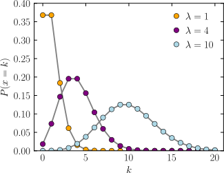
Probability mass function The horizontal axis is the index k, the number of occurrences. λ is the expected rate of occurrences. The vertical axis is the probability of k occurrences given λ. The function is defined only at integer values of k; the connecting lines are only guides for the eye.
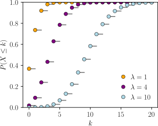
Cumulative distribution function The horizontal axis is the index k, the number of occurrences. The CDF is discontinuous at the integers of k and flat everywhere else because a variable that is Poisson distributed takes on only integer values.
Notation
Parameters	(rate)
Support	${displaystyle kin mathbb {N} _{0}}$ (Natural numbers starting from 0)
PMF	${displaystyle {frac {lambda ^{k}e^{-lambda }}{k!}}}$
CDF	${displaystyle {frac {Gamma (lfloor k+1rfloor ,lambda )}{lfloor krfloor !}},}$ or ${displaystyle e^{-lambda }sum _{j=0}^{lfloor krfloor }{frac {lambda ^{j}}{j!}},}$ or (for where is the upper incomplete gamma function, is the floor function, and is the regularized gamma function)
Mean
Median	${displaystyle approx leftlfloor lambda +{frac {1}{3}}-{frac {1}{50lambda }}rightrfloor }$
Mode
Variance
Skewness	${displaystyle {frac {1}{sqrt {lambda }}}}$
Ex. kurtosis	$frac{1}{lambda}$
Entropy	${displaystyle lambda {Bigl [}1-log(lambda ){Bigr ]}+e^{-lambda }sum _{k=0}^{infty }{frac {lambda ^{k}log(k!)}{k!}}}$ or for large ${displaystyle {begin{aligned}approx {frac {1}{2}}log left(2pi elambda right)-{frac {1}{12lambda }}-{frac {1}{24lambda ^{2}}}\-{frac {19}{360lambda ^{3}}}+{mathcal {O}}left({frac {1}{lambda ^{4}}}right)end{aligned}}}$
MGF	${displaystyle exp left[lambda left(e^{t}-1right)right]}$
CF	${displaystyle exp left[lambda left(e^{it}-1right)right]}$
PGF
Fisher information	$frac{1}{lambda}$

In probability theory and statistics, the Poisson distribution is a discrete probability distribution that expresses the probability of a given number of events occurring in a fixed interval of time or space if these events occur with a known constant mean rate and independently of the time since the last event.^[1] It is named after French mathematician Siméon Denis Poisson (; French pronunciation: [pwasɔ̃]). The Poisson distribution can also be used for the number of events in other specified interval types such as distance, area, or volume.

For instance, a call center receives an average of 180 calls per hour, 24 hours a day. The calls are independent; receiving one does not change the probability of when the next one will arrive. The number of calls received during any minute has a Poisson probability distribution with mean 3: the most likely numbers are 2 and 3 but 1 and 4 are also likely and there is a small probability of it being as low as zero and a very small probability it could be 10.

Another example is the number of decay events that occur from a radioactive source during a defined observation period.

History[edit]

The distribution was first introduced by Siméon Denis Poisson (1781–1840) and published together with his probability theory in his work Recherches sur la probabilité des jugements en matière criminelle et en matière civile (1837).^[2]^: 205-207 The work theorized about the number of wrongful convictions in a given country by focusing on certain random variables N that count, among other things, the number of discrete occurrences (sometimes called «events» or «arrivals») that take place during a time-interval of given length. The result had already been given in 1711 by Abraham de Moivre in De Mensura Sortis seu; de Probabilitate Eventuum in Ludis a Casu Fortuito Pendentibus .^[3]^: 219^[4]^: 14-15^[5]^: 193^[6]^: 157 This makes it an example of Stigler’s law and it has prompted some authors to argue that the Poisson distribution should bear the name of de Moivre.^[7]^[8]

In 1860, Simon Newcomb fitted the Poisson distribution to the number of stars found in a unit of space.^[9]
A further practical application of this distribution was made by Ladislaus Bortkiewicz in 1898 when he was given the task of investigating the number of soldiers in the Prussian army killed accidentally by horse kicks;^[10]^: 23-25 this experiment introduced the Poisson distribution to the field of reliability engineering.

Definitions[edit]

Probability mass function[edit]

A discrete random variable X is said to have a Poisson distribution, with parameter if it has a probability mass function given by:^[11]^: 60

${displaystyle f(k;lambda )=Pr(X{=}k)={frac {lambda ^{k}e^{-lambda }}{k!}},}$

where

The positive real number λ is equal to the expected value of X and also to its variance.^[12]

{displaystyle lambda =operatorname {E} (X)=operatorname {Var} (X).}

The Poisson distribution can be applied to systems with a large number of possible events, each of which is rare. The number of such events that occur during a fixed time interval is, under the right circumstances, a random number with a Poisson distribution.

The equation can be adapted if, instead of the average number of events we are given the average rate at which events occur. Then and:^[13]

${displaystyle P(k{text{ events in interval }}t)={frac {(rt)^{k}e^{-rt}}{k!}}.}$

Example[edit]

Chewing gum on a sidewalk. The number of chewing gums on a single tile is approximately Poisson distributed.

The Poisson distribution may be useful to model events such as:

the number of meteorites greater than 1-meter diameter that strike Earth in a year;
the number of laser photons hitting a detector in a particular time interval; and
the number of students achieving a low and high mark in an exam.

Assumptions and validity[edit]

The Poisson distribution is an appropriate model if the following assumptions are true:^[14]

k is the number of times an event occurs in an interval and k can take values 0, 1, 2, … .
The occurrence of one event does not affect the probability that a second event will occur. That is, events occur independently.
The average rate at which events occur is independent of any occurrences. For simplicity, this is usually assumed to be constant, but may in practice vary with time.
Two events cannot occur at exactly the same instant; instead, at each very small sub-interval, either exactly one event occurs, or no event occurs.

If these conditions are true, then k is a Poisson random variable, and the distribution of k is a Poisson distribution.

The Poisson distribution is also the limit of a binomial distribution, for which the probability of success for each trial equals λ divided by the number of trials, as the number of trials approaches infinity (see Related distributions).

Examples of probability for Poisson distributions[edit]

On a particular river, overflow floods occur once every 100 years on average. Calculate the probability of k = 0, 1, 2, 3, 4, 5, or 6 overflow floods in a 100 year interval, assuming the Poisson model is appropriate.

Because the average event rate is one overflow flood per 100 years, λ = 1

${displaystyle P(k{text{ overflow floods in 100 years}})={frac {lambda ^{k}e^{-lambda }}{k!}}={frac {1^{k}e^{-1}}{k!}}}$

${displaystyle P(k=0{text{ overflow floods in 100 years}})={frac {1^{0}e^{-1}}{0!}}={frac {e^{-1}}{1}}approx 0.368}$

${displaystyle P(k=1{text{ overflow flood in 100 years}})={frac {1^{1}e^{-1}}{1!}}={frac {e^{-1}}{1}}approx 0.368}$

${displaystyle P(k=2{text{ overflow floods in 100 years}})={frac {1^{2}e^{-1}}{2!}}={frac {e^{-1}}{2}}approx 0.184}$

k	P(k overflow floods in 100 years)
0	0.368
1	0.368
2	0.184
3	0.061
4	0.015
5	0.003
6	0.0005

The probability for 0 to 6 overflow floods in a 100 year period.

María Dolores Ugarte and colleagues report that the average number of goals in a World Cup soccer match is approximately 2.5 and the Poisson model is appropriate.^[15]
Because the average event rate is 2.5 goals per match, λ = 2.5 .

${displaystyle P(k{text{ goals in a match}})={frac {2.5^{k}e^{-2.5}}{k!}}}$

${displaystyle P(k=0{text{ goals in a match}})={frac {2.5^{0}e^{-2.5}}{0!}}={frac {e^{-2.5}}{1}}approx 0.082}$

${displaystyle P(k=1{text{ goal in a match}})={frac {2.5^{1}e^{-2.5}}{1!}}={frac {2.5e^{-2.5}}{1}}approx 0.205}$

${displaystyle P(k=2{text{ goals in a match}})={frac {2.5^{2}e^{-2.5}}{2!}}={frac {6.25e^{-2.5}}{2}}approx 0.257}$

k	P(k goals in a World Cup soccer match)
0	0.082
1	0.205
2	0.257
3	0.213
4	0.133
5	0.067
6	0.028
7	0.010

The probability for 0 to 7 goals in a match.

Once in an interval events: The special case of λ = 1 and k = 0[edit]

Suppose that astronomers estimate that large meteorites (above a certain size) hit the earth on average once every 100 years ( λ = 1 event per 100 years), and that the number of meteorite hits follows a Poisson distribution. What is the probability of k = 0 meteorite hits in the next 100 years?

${displaystyle P(k={text{0 meteorites hit in next 100 years}})={frac {1^{0}e^{-1}}{0!}}={frac {1}{e}}approx 0.37.}$

Under these assumptions, the probability that no large meteorites hit the earth in the next 100 years is roughly 0.37. The remaining 1 − 0.37 = 0.63 is the probability of 1, 2, 3, or more large meteorite hits in the next 100 years.
In an example above, an overflow flood occurred once every 100 years (λ = 1). The probability of no overflow floods in 100 years was roughly 0.37, by the same calculation.

In general, if an event occurs on average once per interval (λ = 1), and the events follow a Poisson distribution, then P(0 events in next interval) = 0.37. In addition, P(exactly one event in next interval) = 0.37, as shown in the table for overflow floods.

Examples that violate the Poisson assumptions[edit]

The number of students who arrive at the student union per minute will likely not follow a Poisson distribution, because the rate is not constant (low rate during class time, high rate between class times) and the arrivals of individual students are not independent (students tend to come in groups). The non-constant arrival rate may be modeled as a mixed Poisson distribution, and the arrival of groups rather than individual students as a compound Poisson process.

The number of magnitude 5 earthquakes per year in a country may not follow a Poisson distribution, if one large earthquake increases the probability of aftershocks of similar magnitude.

Examples in which at least one event is guaranteed are not Poisson distributed; but may be modeled using a zero-truncated Poisson distribution.

Count distributions in which the number of intervals with zero events is higher than predicted by a Poisson model may be modeled using a zero-inflated model.

Properties[edit]

Descriptive statistics[edit]

Median[edit]

Bounds for the median () of the distribution are known and are sharp:^[17]

${displaystyle lambda -ln 2leq nu <lambda +{frac {1}{3}}.}$

Higher moments[edit]

The higher non-centered moments, m_k of the Poisson distribution, are Touchard polynomials in λ:

${displaystyle m_{k}=sum _{i=0}^{k}lambda ^{i}{begin{Bmatrix}k\iend{Bmatrix}},}$

where the {braces} denote Stirling numbers of the second kind.^[18]^[1]^: 6 The coefficients of the polynomials have a combinatorial meaning. In fact, when the expected value of the Poisson distribution is 1, then Dobinski’s formula says that the n‑th moment equals the number of partitions of a set of size n.

A simple bound is^[19]

${displaystyle m_{k}=E[X^{k}]leq left({frac {k}{log(k/lambda +1)}}right)^{k}leq lambda ^{k}exp left({frac {k^{2}}{2lambda }}right).}$

Sums of Poisson-distributed random variables[edit]

If ${displaystyle X_{i}sim operatorname {Pois} (lambda _{i})}$ for are independent, then ${textstyle sum _{i=1}^{n}X_{i}sim operatorname {Pois} left(sum _{i=1}^{n}lambda _{i}right).}$ ^[20]^: 65 A converse is Raikov’s theorem, which says that if the sum of two independent random variables is Poisson-distributed, then so are each of those two independent random variables.^[21]^[22]

Other properties[edit]

Poisson races[edit]

Let and be independent random variables, with then we have that

${displaystyle {frac {e^{-({sqrt {mu }}-{sqrt {lambda }})^{2}}}{(lambda +mu )^{2}}}-{frac {e^{-(lambda +mu )}}{2{sqrt {lambda mu }}}}-{frac {e^{-(lambda +mu )}}{4lambda mu }}leq P(X-Ygeq 0)leq e^{-({sqrt {mu }}-{sqrt {lambda }})^{2}}}$

The upper bound is proved using a standard Chernoff bound.

The lower bound can be proved by noting that is the probability that ${textstyle Zgeq {frac {i}{2}},}$ where ${textstyle Zsim operatorname {Bin} left(i,{frac {lambda }{lambda +mu }}right),}$ which is bounded below by ${textstyle {frac {1}{(i+1)^{2}}}e^{-iDleft(0.5|{frac {lambda }{lambda +mu }}right)},}$ where is relative entropy (See the entry on bounds on tails of binomial distributions for details). Further noting that and computing a lower bound on the unconditional probability gives the result. More details can be found in the appendix of Kamath et al..^[27]

[edit]

As a Binomial distribution with infinitesimal time-steps[edit]

The Poisson distribution can be derived as a limiting case to the binomial distribution as the number of trials goes to infinity and the expected number of successes remains fixed — see law of rare events below. Therefore, it can be used as an approximation of the binomial distribution if n is sufficiently large and p is sufficiently small. The Poisson distribution is a good approximation of the binomial distribution if n is at least 20 and p is smaller than or equal to 0.05, and an excellent approximation if n ≥ 100 and n p ≤ 10.^[28]

${displaystyle F_{mathrm {Binomial} }(k;n,p)approx F_{mathrm {Poisson} }(k;lambda =np)}$

General[edit]

If $X_{1}sim mathrm {Pois} (lambda _{1}),$ and $X_{2}sim mathrm {Pois} (lambda _{2}),$ are independent, then the difference $Y=X_{1}-X_{2}$ follows a Skellam distribution.
If $X_{1}sim mathrm {Pois} (lambda _{1}),$ and $X_{2}sim mathrm {Pois} (lambda _{2}),$ are independent, then the distribution of $X_{1}$ conditional on $X_{1}+X_{2}$ is a binomial distribution. Specifically, if ${displaystyle X_{1}+X_{2}=k,}$ then ${displaystyle X_{1}|X_{1}+X_{2}=ksim mathrm {Binom} (k,lambda _{1}/(lambda _{1}+lambda _{2})).}$ More generally, if X₁, X₂, …, X_n are independent Poisson random variables with parameters λ₁, λ₂, …, λ_n then

given $sum _{j=1}^{n}X_{j}=k,$ it follows that ${displaystyle X_{i}{Big |}sum _{j=1}^{n}X_{j}=ksim mathrm {Binom} left(k,{frac {lambda _{i}}{sum _{j=1}^{n}lambda _{j}}}right).}$ In fact, ${displaystyle {X_{i}}sim mathrm {Multinom} left(k,left{{frac {lambda _{i}}{sum _{j=1}^{n}lambda _{j}}}right}right).}$
If and the distribution of conditional on X = k is a binomial distribution, then the distribution of Y follows a Poisson distribution In fact, if, conditional on ${Y_{i}}$ follows a multinomial distribution, ${displaystyle {Y_{i}}mid (X=k)sim mathrm {Multinom} left(k,p_{i}right),}$ then each $Y_{i}$ follows an independent Poisson distribution ${displaystyle Y_{i}sim mathrm {Pois} (lambda cdot p_{i}),rho (Y_{i},Y_{j})=0.}$
The Poisson distribution is a special case of the discrete compound Poisson distribution (or stuttering Poisson distribution) with only a parameter.^[29]^[30] The discrete compound Poisson distribution can be deduced from the limiting distribution of univariate multinomial distribution. It is also a special case of a compound Poisson distribution.
For sufficiently large values of λ, (say λ>1000), the normal distribution with mean λ and variance λ (standard deviation ) is an excellent approximation to the Poisson distribution. If λ is greater than about 10, then the normal distribution is a good approximation if an appropriate continuity correction is performed, i.e., if P(X ≤ x), where x is a non-negative integer, is replaced by P(X ≤ x + 0.5).

${displaystyle F_{mathrm {Poisson} }(x;lambda )approx F_{mathrm {normal} }(x;mu =lambda ,sigma ^{2}=lambda )}$
Variance-stabilizing transformation: If then^[6]^: 168

and^[31]^: 196

Under this transformation, the convergence to normality (as increases) is far faster than the untransformed variable.^{[citation needed]} Other, slightly more complicated, variance stabilizing transformations are available,^[6]^: 168 one of which is Anscombe transform.^[32] See Data transformation (statistics) for more general uses of transformations.
If for every t > 0 the number of arrivals in the time interval [0, t] follows the Poisson distribution with mean λt, then the sequence of inter-arrival times are independent and identically distributed exponential random variables having mean 1/λ.^[33]^{: 317–319}
The cumulative distribution functions of the Poisson and chi-squared distributions are related in the following ways:^[6]^: 167

${displaystyle F_{text{Poisson}}(k;lambda )=1-F_{chi ^{2}}(2lambda ;2(k+1))quad quad {text{ integer }}k,}$

and^[6]^: 158

${displaystyle P(X=k)=F_{chi ^{2}}(2lambda ;2(k+1))-F_{chi ^{2}}(2lambda ;2k).}$

Poisson approximation[edit]

Assume ${displaystyle X_{1}sim operatorname {Pois} (lambda _{1}),X_{2}sim operatorname {Pois} (lambda _{2}),dots ,X_{n}sim operatorname {Pois} (lambda _{n})}$ where ${displaystyle lambda _{1}+lambda _{2}+dots +lambda _{n}=1,}$ then^[34] ${displaystyle (X_{1},X_{2},dots ,X_{n})}$ is multinomially distributed
${displaystyle (X_{1},X_{2},dots ,X_{n})sim operatorname {Mult} (N,lambda _{1},lambda _{2},dots ,lambda _{n})}$ conditioned on ${displaystyle N=X_{1}+X_{2}+dots X_{n}.}$

This means^[25]^: 101-102, among other things, that for any nonnegative function
if ${displaystyle (Y_{1},Y_{2},dots ,Y_{n})sim operatorname {Mult} (m,mathbf {p} )}$ is multinomially distributed, then

${displaystyle operatorname {E} [f(Y_{1},Y_{2},dots ,Y_{n})]leq e{sqrt {m}}operatorname {E} [f(X_{1},X_{2},dots ,X_{n})]}$

where ${displaystyle (X_{1},X_{2},dots ,X_{n})sim operatorname {Pois} (mathbf {p} ).}$

The factor of can be replaced by 2 if is further assumed to be monotonically increasing or decreasing.

Bivariate Poisson distribution[edit]

This distribution has been extended to the bivariate case.^[35] The generating function for this distribution is

${displaystyle g(u,v)=exp[(theta _{1}-theta _{12})(u-1)+(theta _{2}-theta _{12})(v-1)+theta _{12}(uv-1)]}$

with

${displaystyle theta _{1},theta _{2}>theta _{12}>0}$

The marginal distributions are Poisson(θ₁) and Poisson(θ₂) and the correlation coefficient is limited to the range

${displaystyle 0leq rho leq min left{{sqrt {frac {theta _{1}}{theta _{2}}}},{sqrt {frac {theta _{2}}{theta _{1}}}}right}}$

A simple way to generate a bivariate Poisson distribution $X_{1},X_{2}$ is to take three independent Poisson distributions $Y_{1},Y_{2},Y_{3}$ with means $lambda _{1},lambda _{2},lambda _{3}$ and then set ${displaystyle X_{1}=Y_{1}+Y_{3},X_{2}=Y_{2}+Y_{3}.}$ The probability function of the bivariate Poisson distribution is

${displaystyle Pr(X_{1}=k_{1},X_{2}=k_{2})=exp left(-lambda _{1}-lambda _{2}-lambda _{3}right){frac {lambda _{1}^{k_{1}}}{k_{1}!}}{frac {lambda _{2}^{k_{2}}}{k_{2}!}}sum _{k=0}^{min(k_{1},k_{2})}{binom {k_{1}}{k}}{binom {k_{2}}{k}}k!left({frac {lambda _{3}}{lambda _{1}lambda _{2}}}right)^{k}}$

Free Poisson distribution[edit]

The free Poisson distribution^[36] with jump size alpha and rate lambda arises in free probability theory as the limit of repeated free convolution

${displaystyle left(left(1-{frac {lambda }{N}}right)delta _{0}+{frac {lambda }{N}}delta _{alpha }right)^{boxplus N}}$

as N → ∞.

In other words, let $X_{N}$ be random variables so that $X_{N}$ has value alpha with probability ${textstyle {frac {lambda }{N}}}$ and value 0 with the remaining probability. Assume also that the family $X_{1},X_{2},ldots$ are freely independent. Then the limit as of the law of ${displaystyle X_{1}+cdots +X_{N}}$ is given by the Free Poisson law with parameters

This definition is analogous to one of the ways in which the classical Poisson distribution is obtained from a (classical) Poisson process.

The measure associated to the free Poisson law is given by^[37]

${displaystyle mu ={begin{cases}(1-lambda )delta _{0}+lambda nu ,&{text{if }}0leq lambda leq 1\nu ,&{text{if }}lambda >1,end{cases}}}$

where

${displaystyle nu ={frac {1}{2pi alpha t}}{sqrt {4lambda alpha ^{2}-(t-alpha (1+lambda ))^{2}}},dt}$

and has support ${displaystyle [alpha (1-{sqrt {lambda }})^{2},alpha (1+{sqrt {lambda }})^{2}].}$

This law also arises in random matrix theory as the Marchenko–Pastur law. Its free cumulants are equal to ${displaystyle kappa _{n}=lambda alpha ^{n}.}$

Some transforms of this law[edit]

We give values of some important transforms of the free Poisson law; the computation can be found in e.g. in the book Lectures on the Combinatorics of Free Probability by A. Nica and R. Speicher^[38]

The R-transform of the free Poisson law is given by

${displaystyle R(z)={frac {lambda alpha }{1-alpha z}}.}$

The Cauchy transform (which is the negative of the Stieltjes transformation) is given by

${displaystyle G(z)={frac {z+alpha -lambda alpha -{sqrt {(z-alpha (1+lambda ))^{2}-4lambda alpha ^{2}}}}{2alpha z}}}$

The S-transform is given by

${displaystyle S(z)={frac {1}{z+lambda }}}$

in the case that

Weibull and Stable count[edit]

Poisson’s probability mass function can be expressed in a form similar to the product distribution of a Weibull distribution and a variant form of the stable count distribution.
The variable can be regarded as inverse of Lévy’s stability parameter in the stable count distribution:

${displaystyle f(k;lambda )=displaystyle int _{0}^{infty }{frac {1}{u}},W_{k+1}({frac {lambda }{u}})left[left(k+1right)u^{k},{mathfrak {N}}_{frac {1}{k+1}}left(u^{k+1}right)right],du,}$

where ${displaystyle {mathfrak {N}}_{alpha }(nu )}$ is a standard stable count distribution of shape and ${displaystyle W_{k+1}(x)}$ is a standard Weibull distribution of shape

Statistical inference[edit]

Parameter estimation[edit]

Given a sample of n measured values ${displaystyle k_{i}in {0,1,dots },}$ for i = 1, …, n, we wish to estimate the value of the parameter λ of the Poisson population from which the sample was drawn. The maximum likelihood estimate is ^[39]

${displaystyle {widehat {lambda }}_{mathrm {MLE} }={frac {1}{n}}sum _{i=1}^{n}k_{i} .}$

Since each observation has expectation λ so does the sample mean. Therefore, the maximum likelihood estimate is an unbiased estimator of λ. It is also an efficient estimator since its variance achieves the Cramér–Rao lower bound (CRLB).^[40] Hence it is minimum-variance unbiased. Also it can be proven that the sum (and hence the sample mean as it is a one-to-one function of the sum) is a complete and sufficient statistic for λ.

To prove sufficiency we may use the factorization theorem. Consider partitioning the probability mass function of the joint Poisson distribution for the sample into two parts: one that depends solely on the sample (called ) and one that depends on the parameter lambda and the sample only through the function Then is a sufficient statistic for

${displaystyle P(mathbf {x} )=prod _{i=1}^{n}{frac {lambda ^{x_{i}}e^{-lambda }}{x_{i}!}}={frac {1}{prod _{i=1}^{n}x_{i}!}}times lambda ^{sum _{i=1}^{n}x_{i}}e^{-nlambda }}$

The first term, depends only on The second term, depends on the sample only through ${textstyle T(mathbf {x} )=sum _{i=1}^{n}x_{i}.}$ Thus, is sufficient.

To find the parameter λ that maximizes the probability function for the Poisson population, we can use the logarithm of the likelihood function:

${displaystyle {begin{aligned}ell (lambda )&=ln prod _{i=1}^{n}f(k_{i}mid lambda )\&=sum _{i=1}^{n}ln !left({frac {e^{-lambda }lambda ^{k_{i}}}{k_{i}!}}right)\&=-nlambda +left(sum _{i=1}^{n}k_{i}right)ln(lambda )-sum _{i=1}^{n}ln(k_{i}!).end{aligned}}}$

We take the derivative of ell with respect to λ and compare it to zero:

${displaystyle {frac {mathrm {d} }{mathrm {d} lambda }}ell (lambda )=0iff -n+left(sum _{i=1}^{n}k_{i}right){frac {1}{lambda }}=0.!}$

Solving for λ gives a stationary point.

$lambda ={frac {sum _{i=1}^{n}k_{i}}{n}}$

So λ is the average of the k_i values. Obtaining the sign of the second derivative of L at the stationary point will determine what kind of extreme value λ is.

${displaystyle {frac {partial ^{2}ell }{partial lambda ^{2}}}=-lambda ^{-2}sum _{i=1}^{n}k_{i}}$

Evaluating the second derivative at the stationary point gives:

${displaystyle {frac {partial ^{2}ell }{partial lambda ^{2}}}=-{frac {n^{2}}{sum _{i=1}^{n}k_{i}}}}$

which is the negative of n times the reciprocal of the average of the k_i. This expression is negative when the average is positive. If this is satisfied, then the stationary point maximizes the probability function.

For completeness, a family of distributions is said to be complete if and only if implies that $P_{lambda }(g(T)=0)=1$ for all If the individual $X_{i}$ are iid then ${textstyle T(mathbf {x} )=sum _{i=1}^{n}X_{i}sim mathrm {Po} (nlambda ).}$ Knowing the distribution we want to investigate, it is easy to see that the statistic is complete.

${displaystyle E(g(T))=sum _{t=0}^{infty }g(t){frac {(nlambda )^{t}e^{-nlambda }}{t!}}=0}$

For this equality to hold, g(t) must be 0. This follows from the fact that none of the other terms will be 0 for all in the sum and for all possible values of Hence, for all lambda implies that ${displaystyle P_{lambda }(g(T)=0)=1,}$ and the statistic has been shown to be complete.

Confidence interval[edit]

The confidence interval for the mean of a Poisson distribution can be expressed using the relationship between the cumulative distribution functions of the Poisson and chi-squared distributions. The chi-squared distribution is itself closely related to the gamma distribution, and this leads to an alternative expression. Given an observation k from a Poisson distribution with mean μ, a confidence interval for μ with confidence level 1 – α is

${displaystyle {tfrac {1}{2}}chi ^{2}(alpha /2;2k)leq mu leq {tfrac {1}{2}}chi ^{2}(1-alpha /2;2k+2),}$

or equivalently,

$F^{-1}(alpha /2;k,1)leq mu leq F^{-1}(1-alpha /2;k+1,1),$

where $chi ^{2}(p;n)$ is the quantile function (corresponding to a lower tail area p) of the chi-squared distribution with n degrees of freedom and $F^{-1}(p;n,1)$ is the quantile function of a gamma distribution with shape parameter n and scale parameter 1.^[6]^: 176-178^[41] This interval is ‘exact’ in the sense that its coverage probability is never less than the nominal 1 – α.

When quantiles of the gamma distribution are not available, an accurate approximation to this exact interval has been proposed (based on the Wilson–Hilferty transformation):^[42]

$kleft(1-{frac {1}{9k}}-{frac {z_{alpha /2}}{3{sqrt {k}}}}right)^{3}leq mu leq (k+1)left(1-{frac {1}{9(k+1)}}+{frac {z_{alpha /2}}{3{sqrt {k+1}}}}right)^{3},$

where $z_{alpha /2}$ denotes the standard normal deviate with upper tail area α / 2.

For application of these formulae in the same context as above (given a sample of n measured values k_i each drawn from a Poisson distribution with mean λ), one would set

${displaystyle k=sum _{i=1}^{n}k_{i},}$

calculate an interval for μ = n λ , and then derive the interval for λ.

Bayesian inference[edit]

In Bayesian inference, the conjugate prior for the rate parameter λ of the Poisson distribution is the gamma distribution.^[43] Let

{displaystyle lambda sim mathrm {Gamma} (alpha ,beta )}

denote that λ is distributed according to the gamma density g parameterized in terms of a shape parameter α and an inverse scale parameter β:

$g(lambda mid alpha ,beta )={frac {beta ^{alpha }}{Gamma (alpha )}};lambda ^{alpha -1};e^{-beta ,lambda }qquad {text{ for }}lambda >0,!.$

Then, given the same sample of n measured values k_i as before, and a prior of Gamma(α, β), the posterior distribution is

${displaystyle lambda sim mathrm {Gamma} left(alpha +sum _{i=1}^{n}k_{i},beta +nright).}$

Note that the posterior mean is linear and is given by

${displaystyle E[lambda |k_{1},ldots ,k_{n}]={frac {alpha +sum _{i=1}^{n}k_{i}}{beta +n}}.}$

It can be shown that gamma distribution is the only prior that induces linearity of the conditional mean. Moreover, a converse result exists which states that if the conditional mean is close to a linear function in the $L_{2}$ distance than the prior distribution of λ must be close to gamma distribution in Levy distance.^[44]

The posterior mean E[λ] approaches the maximum likelihood estimate ${widehat {lambda }}_{mathrm {MLE} }$ in the limit as which follows immediately from the general expression of the mean of the gamma distribution.

The posterior predictive distribution for a single additional observation is a negative binomial distribution,^[45]^: 53 sometimes called a gamma–Poisson distribution.

Simultaneous estimation of multiple Poisson means[edit]

Suppose $X_{1},X_{2},dots ,X_{p}$ is a set of independent random variables from a set of Poisson distributions, each with a parameter and we would like to estimate these parameters. Then, Clevenson and Zidek show that under the normalized squared error loss ${textstyle L(lambda ,{hat {lambda }})=sum _{i=1}^{p}lambda _{i}^{-1}({hat {lambda }}_{i}-lambda _{i})^{2},}$ when then, similar as in Stein’s example for the Normal means, the MLE estimator ${hat {lambda }}_{i}=X_{i}$ is inadmissible. ^[46]

In this case, a family of minimax estimators is given for any and $bgeq (p-2+p^{-1})$ as^[47]

${hat {lambda }}_{i}=left(1-{frac {c}{b+sum _{i=1}^{p}X_{i}}}right)X_{i},qquad i=1,dots ,p.$

Occurrence and applications[edit]

Applications of the Poisson distribution can be found in many fields including:^[48]

Count data in general
Telecommunication example: telephone calls arriving in a system.
Astronomy example: photons arriving at a telescope.
Chemistry example: the molar mass distribution of a living polymerization.^[49]
Biology example: the number of mutations on a strand of DNA per unit length.
Management example: customers arriving at a counter or call centre.
Finance and insurance example: number of losses or claims occurring in a given period of time.
Earthquake seismology example: an asymptotic Poisson model of seismic risk for large earthquakes.^[50]
Radioactivity example: number of decays in a given time interval in a radioactive sample.
Optics example: the number of photons emitted in a single laser pulse. This is a major vulnerability to most Quantum key distribution protocols known as Photon Number Splitting (PNS).

The Poisson distribution arises in connection with Poisson processes. It applies to various phenomena of discrete properties (that is, those that may happen 0, 1, 2, 3, … times during a given period of time or in a given area) whenever the probability of the phenomenon happening is constant in time or space. Examples of events that may be modelled as a Poisson distribution include:

The number of soldiers killed by horse-kicks each year in each corps in the Prussian cavalry. This example was used in a book by Ladislaus Bortkiewicz (1868–1931).^[10]^: 23-25
The number of yeast cells used when brewing Guinness beer. This example was used by William Sealy Gosset (1876–1937).^[51]^[52]
The number of phone calls arriving at a call centre within a minute. This example was described by A.K. Erlang (1878–1929).^[53]
Internet traffic.
The number of goals in sports involving two competing teams.^[54]
The number of deaths per year in a given age group.
The number of jumps in a stock price in a given time interval.
Under an assumption of homogeneity, the number of times a web server is accessed per minute.
The number of mutations in a given stretch of DNA after a certain amount of radiation.
The proportion of cells that will be infected at a given multiplicity of infection.
The number of bacteria in a certain amount of liquid.^[55]
The arrival of photons on a pixel circuit at a given illumination and over a given time period.
The targeting of V-1 flying bombs on London during World War II investigated by R. D. Clarke in 1946.^[56]

Gallagher showed in 1976 that the counts of prime numbers in short intervals obey a Poisson distribution^[57] provided a certain version of the unproved prime r-tuple conjecture of Hardy-Littlewood^[58] is true.

Law of rare events[edit]

Comparison of the Poisson distribution (black lines) and the binomial distribution with n = 10 (red circles), n = 20 (blue circles), n = 1000 (green circles). All distributions have a mean of 5. The horizontal axis shows the number of events k. As n gets larger, the Poisson distribution becomes an increasingly better approximation for the binomial distribution with the same mean.

The rate of an event is related to the probability of an event occurring in some small subinterval (of time, space or otherwise). In the case of the Poisson distribution, one assumes that there exists a small enough subinterval for which the probability of an event occurring twice is «negligible». With this assumption one can derive the Poisson distribution from the Binomial one, given only the information of expected number of total events in the whole interval.

Let the total number of events in the whole interval be denoted by Divide the whole interval into subintervals $I_{1},dots ,I_{n}$ of equal size, such that (since we are interested in only very small portions of the interval this assumption is meaningful). This means that the expected number of events in each of the n subintervals is equal to

Now we assume that the occurrence of an event in the whole interval can be seen as a sequence of n Bernoulli trials, where the -th Bernoulli trial corresponds to looking whether an event happens at the subinterval $I_{i}$ with probability The expected number of total events in such trials would be the expected number of total events in the whole interval. Hence for each subdivision of the interval we have approximated the occurrence of the event as a Bernoulli process of the form As we have noted before we want to consider only very small subintervals. Therefore, we take the limit as goes to infinity.

In this case the binomial distribution converges to what is known as the Poisson distribution by the Poisson limit theorem.

In several of the above examples — such as, the number of mutations in a given sequence of DNA—the events being counted are actually the outcomes of discrete trials, and would more precisely be modelled using the binomial distribution, that is

In such cases n is very large and p is very small (and so the expectation n p is of intermediate magnitude). Then the distribution may be approximated by the less cumbersome Poisson distribution

This approximation is sometimes known as the law of rare events,^[59]^: 5 since each of the n individual Bernoulli events rarely occurs.

The name «law of rare events» may be misleading because the total count of success events in a Poisson process need not be rare if the parameter n p is not small. For example, the number of telephone calls to a busy switchboard in one hour follows a Poisson distribution with the events appearing frequent to the operator, but they are rare from the point of view of the average member of the population who is very unlikely to make a call to that switchboard in that hour.

The variance of the binomial distribution is 1 − p times that of the Poisson distribution, so almost equal when p is very small.

The word law is sometimes used as a synonym of probability distribution, and convergence in law means convergence in distribution. Accordingly, the Poisson distribution is sometimes called the «law of small numbers» because it is the probability distribution of the number of occurrences of an event that happens rarely but has very many opportunities to happen. The Law of Small Numbers is a book by Ladislaus Bortkiewicz about the Poisson distribution, published in 1898.^[10]^[60]

Poisson point process[edit]

The Poisson distribution arises as the number of points of a Poisson point process located in some finite region. More specifically, if D is some region space, for example Euclidean space R^d, for which |D|, the area, volume or, more generally, the Lebesgue measure of the region is finite, and if N(D) denotes the number of points in D, then

$P(N(D)=k)={frac {(lambda |D|)^{k}e^{-lambda |D|}}{k!}}.$

Poisson regression and negative binomial regression[edit]

Poisson regression and negative binomial regression are useful for analyses where the dependent (response) variable is the count (0, 1, 2, … ) of the number of events or occurrences in an interval.

Other applications in science[edit]

In a Poisson process, the number of observed occurrences fluctuates about its mean λ with a standard deviation ${displaystyle sigma _{k}={sqrt {lambda }}.}$ These fluctuations are denoted as Poisson noise or (particularly in electronics) as shot noise.

The correlation of the mean and standard deviation in counting independent discrete occurrences is useful scientifically. By monitoring how the fluctuations vary with the mean signal, one can estimate the contribution of a single occurrence, even if that contribution is too small to be detected directly. For example, the charge e on an electron can be estimated by correlating the magnitude of an electric current with its shot noise. If N electrons pass a point in a given time t on the average, the mean current is I=eN/t ; since the current fluctuations should be of the order ${displaystyle sigma _{I}=e{sqrt {N}}/t}$ (i.e., the standard deviation of the Poisson process), the charge can be estimated from the ratio ${displaystyle tsigma _{I}^{2}/I.}$ ^{[citation needed]}

An everyday example is the graininess that appears as photographs are enlarged; the graininess is due to Poisson fluctuations in the number of reduced silver grains, not to the individual grains themselves. By correlating the graininess with the degree of enlargement, one can estimate the contribution of an individual grain (which is otherwise too small to be seen unaided).^{[citation needed]} Many other molecular applications of Poisson noise have been developed, e.g., estimating the number density of receptor molecules in a cell membrane.

${displaystyle Pr(N_{t}=k)=f(k;lambda t)={frac {(lambda t)^{k}e^{-lambda t}}{k!}}.}$

In causal set theory the discrete elements of spacetime follow a Poisson distribution in the volume.

Computational methods[edit]

The Poisson distribution poses two different tasks for dedicated software libraries: evaluating the distribution , and drawing random numbers according to that distribution.

Evaluating the Poisson distribution[edit]

Computing for given and lambda is a trivial task that can be accomplished by using the standard definition of in terms of exponential, power, and factorial functions. However, the conventional definition of the Poisson distribution contains two terms that can easily overflow on computers: λ^k and k!. The fraction of λ^k to k! can also produce a rounding error that is very large compared to e^−λ, and therefore give an erroneous result. For numerical stability the Poisson probability mass function should therefore be evaluated as

{displaystyle !f(k;lambda )=exp left[kln lambda -lambda -ln Gamma (k+1)right],}

which is mathematically equivalent but numerically stable. The natural logarithm of the Gamma function can be obtained using the lgamma function in the C standard library (C99 version) or R, the gammaln function in MATLAB or SciPy, or the log_gamma function in Fortran 2008 and later.

Some computing languages provide built-in functions to evaluate the Poisson distribution, namely

Random variate generation[edit]

The less trivial task is to draw integer random variate from the Poisson distribution with given

Solutions are provided by:

R: function rpois(n, lambda);
GNU Scientific Library (GSL): function gsl_ran_poisson

A simple algorithm to generate random Poisson-distributed numbers (pseudo-random number sampling) has been given by Knuth:^[63]^: 137-138

algorithm poisson random number (Knuth):
    init:
        Let L ← e^−λ, k ← 0 and p ← 1.
    do:
        k ← k + 1.
        Generate uniform random number u in [0,1] and let p ← p × u.
    while p > L.
    return k − 1.

The complexity is linear in the returned value k, which is λ on average. There are many other algorithms to improve this. Some are given in Ahrens & Dieter, see § References below.

For large values of λ, the value of L = e^−λ may be so small that it is hard to represent. This can be solved by a change to the algorithm which uses an additional parameter STEP such that e^−STEP does not underflow:^{[citation needed]}

algorithm poisson random number (Junhao, based on Knuth):
    init:
        Let λLeft ← λ, k ← 0 and p ← 1.
    do:
        k ← k + 1.
        Generate uniform random number u in (0,1) and let p ← p × u.
        while p < 1 and λLeft > 0:
            if λLeft > STEP:
                p ← p × e^STEP
                λLeft ← λLeft − STEP
            else:
                p ← p × e^λLeft
                λLeft ← 0
    while p > 1.
    return k − 1.

The choice of STEP depends on the threshold of overflow. For double precision floating point format the threshold is near e⁷⁰⁰, so 500 should be a safe STEP.

Other solutions for large values of λ include rejection sampling and using Gaussian approximation.

Inverse transform sampling is simple and efficient for small values of λ, and requires only one uniform random number u per sample. Cumulative probabilities are examined in turn until one exceeds u.

algorithm Poisson generator based upon the inversion by sequential search:^[64]^: 505
    init:
        Let x ← 0, p ← e^−λ, s ← p.
        Generate uniform random number u in [0,1].
    while u > s do:
        x ← x + 1.
        p ← p × λ / x.
        s ← s + p.
    return x.

References[edit]

Citations[edit]

^ ^a ^b
Haight, Frank A. (1967). Handbook of the Poisson Distribution. New York, NY, US: John Wiley & Sons. ISBN 978-0-471-33932-8.
^
Poisson, Siméon D. (1837). Probabilité des jugements en matière criminelle et en matière civile, précédées des règles générales du calcul des probabilités [Research on the Probability of Judgments in Criminal and Civil Matters] (in French). Paris, France: Bachelier.
^
de Moivre, Abraham (1711). «De mensura sortis, seu, de probabilitate eventuum in ludis a casu fortuito pendentibus» [On the Measurement of Chance, or, on the Probability of Events in Games Depending Upon Fortuitous Chance]. Philosophical Transactions of the Royal Society (in Latin). 27 (329): 213–264. doi:10.1098/rstl.1710.0018.
^
de Moivre, Abraham (1718). The Doctrine of Chances: Or, A Method of Calculating the Probability of Events in Play. London, Great Britain: W. Pearson. ISBN 9780598843753.
^
de Moivre, Abraham (1721). «Of the Laws of Chance». In Motte, Benjamin (ed.). The Philosophical Transactions from the Year MDCC (where Mr. Lowthorp Ends) to the Year MDCCXX. Abridg’d, and Dispos’d Under General Heads (in Latin). Vol. I. London, Great Britain: R. Wilkin, R. Robinson, S. Ballard, W. and J. Innys, and J. Osborn. pp. 190–219.
^ ^a ^b ^c ^d ^e ^f ^g ^h ⁱ
Johnson, Norman L.; Kemp, Adrienne W.; Kotz, Samuel (2005). «Poisson Distribution». Univariate Discrete Distributions (3rd ed.). New York, NY, US: John Wiley & Sons, Inc. pp. 156–207. doi:10.1002/0471715816. ISBN 978-0-471-27246-5.
^
Stigler, Stephen M. (1982). «Poisson on the Poisson Distribution». Statistics & Probability Letters. 1 (1): 33–35. doi:10.1016/0167-7152(82)90010-4.
^
Hald, Anders; de Moivre, Abraham; McClintock, Bruce (1984). «A. de Moivre: ‘De Mensura Sortis’ or ‘On the Measurement of Chance’«. International Statistical Review / Revue Internationale de Statistique. 52 (3): 229–262. doi:10.2307/1403045. JSTOR 1403045.
^
Newcomb, Simon (1860). «Notes on the theory of probabilities». The Mathematical Monthly. 2 (4): 134–140.
^ ^a ^b ^c
von Bortkiewitsch, Ladislaus (1898). Das Gesetz der kleinen Zahlen [The law of small numbers] (in German). Leipzig, Germany: B.G. Teubner. pp. 1, 23–25.

On page 1, Bortkiewicz presents the Poisson distribution.

On pages 23–25, Bortkiewitsch presents his analysis of «4. Beispiel: Die durch Schlag eines Pferdes im preußischen Heere Getöteten.» [4. Example: Those killed in the Prussian army by a horse’s kick.]
^
Yates, Roy D.; Goodman, David J. (2014). Probability and Stochastic Processes: A Friendly Introduction for Electrical and Computer Engineers (2nd ed.). Hoboken, NJ: Wiley. ISBN 978-0-471-45259-1.
^ For the proof, see:
Proof wiki: expectation and Proof wiki: variance
^ Kardar, Mehran (2007). Statistical Physics of Particles. Cambridge University Press. p. 42. ISBN 978-0-521-87342-0. OCLC 860391091.
^
Koehrsen, William (2019-01-20). The Poisson Distribution and Poisson Process Explained. Towards Data Science. Retrieved 2019-09-19.
^
Ugarte, M.D.; Militino, A.F.; Arnholt, A.T. (2016). Probability and Statistics with R (2nd ed.). Boca Raton, FL, US: CRC Press. ISBN 978-1-4665-0439-4.
^
Helske, Jouni (2017). «KFAS: Exponential Family State Space Models in R». Journal of Statistical Software. 78 (10). arXiv:1612.01907. doi:10.18637/jss.v078.i10. S2CID 14379617.
^
Choi, Kwok P. (1994). «On the medians of gamma distributions and an equation of Ramanujan». Proceedings of the American Mathematical Society. 121 (1): 245–251. doi:10.2307/2160389. JSTOR 2160389.
^
Riordan, John (1937). «Moment Recurrence Relations for Binomial, Poisson and Hypergeometric Frequency Distributions» (PDF). Annals of Mathematical Statistics. 8 (2): 103–111. doi:10.1214/aoms/1177732430. JSTOR 2957598.
^ D. Ahle, Thomas (2022). «Sharp and simple bounds for the raw moments of the Binomial and Poisson distributions». Statistics & Probability Letters. 182: 109306. arXiv:2103.17027. doi:10.1016/j.spl.2021.109306.
^
Lehmann, Erich Leo (1986). Testing Statistical Hypotheses (2nd ed.). New York, NJ, US: Springer Verlag. ISBN 978-0-387-94919-2.
^
Raikov, Dmitry (1937). «On the decomposition of Poisson laws». Comptes Rendus de l’Académie des Sciences de l’URSS. 14: 9–11.
^
von Mises, Richard (1964). Mathematical Theory of Probability and Statistics. New York, NJ, US: Academic Press. doi:10.1016/C2013-0-12460-9. ISBN 978-1-4832-3213-3.
^
Laha, Radha G.; Rohatgi, Vijay K. (1979). Probability Theory. New York, NJ, US: John Wiley & Sons. ISBN 978-0-471-03262-5.
^ Mitzenmacher, Michael (2017). Probability and computing: Randomization and probabilistic techniques in algorithms and data analysis. Eli Upfal (2nd ed.). Cambridge, UK. Exercise 5.14. ISBN 978-1-107-15488-9. OCLC 960841613.
^ ^a ^b
Mitzenmacher, Michael; Upfal, Eli (2005). Probability and Computing: Randomized Algorithms and Probabilistic Analysis. Cambridge, UK: Cambridge University Press. ISBN 978-0-521-83540-4.
^ ^a ^b
Short, Michael (2013). «Improved Inequalities for the Poisson and Binomial Distribution and Upper Tail Quantile Functions». ISRN Probability and Statistics. 2013: 412958. doi:10.1155/2013/412958.
^
Kamath, Govinda M.; Şaşoğlu, Eren; Tse, David (14–19 June 2015). Optimal haplotype assembly from high-throughput mate-pair reads. 2015 IEEE International Symposium on Information Theory (ISIT). Hong Kong, China. pp. 914–918. arXiv:1502.01975. doi:10.1109/ISIT.2015.7282588. S2CID 128634.
^
Prins, Jack (2012). «6.3.3.1. Counts Control Charts». e-Handbook of Statistical Methods. NIST/SEMATECH. Retrieved 2019-09-20.
^
Zhang, Huiming; Liu, Yunxiao; Li, Bo (2014). «Notes on discrete compound Poisson model with applications to risk theory». Insurance: Mathematics and Economics. 59: 325–336. doi:10.1016/j.insmatheco.2014.09.012.
^
Zhang, Huiming; Li, Bo (2016). «Characterizations of discrete compound Poisson distributions». Communications in Statistics — Theory and Methods. 45 (22): 6789–6802. doi:10.1080/03610926.2014.901375. S2CID 125475756.
^
McCullagh, Peter; Nelder, John (1989). Generalized Linear Models. Monographs on Statistics and Applied Probability. Vol. 37. London, UK: Chapman and Hall. ISBN 978-0-412-31760-6.
^
Anscombe, Francis J. (1948). «The transformation of Poisson, binomial and negative binomial data». Biometrika. 35 (3–4): 246–254. doi:10.1093/biomet/35.3-4.246. JSTOR 2332343.
^
Ross, Sheldon M. (2010). Introduction to Probability Models (10th ed.). Boston, MA: Academic Press. ISBN 978-0-12-375686-2.
^ «1.7.7 – Relationship between the Multinomial and Poisson | STAT 504».
^
Loukas, Sotirios; Kemp, C. David (1986). «The Index of Dispersion Test for the Bivariate Poisson Distribution». Biometrics. 42 (4): 941–948. doi:10.2307/2530708. JSTOR 2530708.
^ Free Random Variables by D. Voiculescu, K. Dykema, A. Nica, CRM Monograph Series, American Mathematical Society, Providence RI, 1992
^ James A. Mingo, Roland Speicher: Free Probability and Random Matrices. Fields Institute Monographs, Vol. 35, Springer, New York, 2017.
^ Lectures on the Combinatorics of Free Probability by A. Nica and R. Speicher, pp. 203–204, Cambridge Univ. Press 2006
^ Paszek, Ewa. «Maximum likelihood estimation – examples». cnx.org.
^ Van Trees, Harry L. (2013). Detection estimation and modulation theory. Kristine L. Bell, Zhi Tian (Second ed.). Hoboken, N.J. ISBN 978-1-299-66515-6. OCLC 851161356.
^
Garwood, Frank (1936). «Fiducial Limits for the Poisson Distribution». Biometrika. 28 (3/4): 437–442. doi:10.1093/biomet/28.3-4.437. JSTOR 2333958.
^
Breslow, Norman E.; Day, Nick E. (1987). Statistical Methods in Cancer Research. Vol. 2 — The Design and Analysis of Cohort Studies. Lyon, France: International Agency for Research on Cancer. ISBN 978-92-832-0182-3. Archived from the original on 2018-08-08. Retrieved 2012-03-11.
^
Fink, Daniel (1997). A Compendium of Conjugate Priors.
^ Dytso, Alex; Poor, H. Vincent (2020). «Estimation in Poisson noise: Properties of the conditional mean estimator». IEEE Transactions on Information Theory. 66 (7): 4304–4323. doi:10.1109/TIT.2020.2979978. S2CID 207853178.
^
Gelman; Carlin, John B.; Stern, Hal S.; Rubin, Donald B. (2003). Bayesian Data Analysis (2nd ed.). Boca Raton, FL, US: Chapman & Hall/CRC. ISBN 1-58488-388-X.
^
Clevenson, M. Lawrence; Zidek, James V. (1975). «Simultaneous estimation of the means of independent Poisson laws». Journal of the American Statistical Association. 70 (351): 698–705. doi:10.1080/01621459.1975.10482497. JSTOR 2285958.
^
Berger, James O. (1985). Statistical Decision Theory and Bayesian Analysis. Springer Series in Statistics (2nd ed.). New York, NY: Springer-Verlag. Bibcode:1985sdtb.book…..B. doi:10.1007/978-1-4757-4286-2. ISBN 978-0-387-96098-2.
^
Rasch, Georg (1963). The Poisson Process as a Model for a Diversity of Behavioural Phenomena (PDF). 17th International Congress of Psychology. Vol. 2. Washington, DC: American Psychological Association. doi:10.1037/e685262012-108.
^
Flory, Paul J. (1940). «Molecular Size Distribution in Ethylene Oxide Polymers». Journal of the American Chemical Society. 62 (6): 1561–1565. doi:10.1021/ja01863a066.
^
Lomnitz, Cinna (1994). Fundamentals of Earthquake Prediction. New York, NY: John Wiley & Sons. ISBN 0-471-57419-8. OCLC 647404423.
^
a student (1907). «On the error of counting with a haemacytometer». Biometrika. 5 (3): 351–360. doi:10.2307/2331633. JSTOR 2331633.
^
Boland, Philip J. (1984). «A biographical glimpse of William Sealy Gosset». The American Statistician. 38 (3): 179–183. doi:10.1080/00031305.1984.10483195. JSTOR 2683648.
^
Erlang, Agner K. (1909). «Sandsynlighedsregning og Telefonsamtaler» [Probability Calculation and Telephone Conversations]. Nyt Tidsskrift for Matematik (in Danish). 20 (B): 33–39. JSTOR 24528622.
^
Hornby, Dave (2014). «Football Prediction Model: Poisson Distribution». Sports Betting Online. Retrieved 2014-09-19.
^
Koyama, Kento; Hokunan, Hidekazu; Hasegawa, Mayumi; Kawamura, Shuso; Koseki, Shigenobu (2016). «Do bacterial cell numbers follow a theoretical Poisson distribution? Comparison of experimentally obtained numbers of single cells with random number generation via computer simulation». Food Microbiology. 60: 49–53. doi:10.1016/j.fm.2016.05.019. PMID 27554145.
^
Clarke, R. D. (1946). «An application of the Poisson distribution» (PDF). Journal of the Institute of Actuaries. 72 (3): 481. doi:10.1017/S0020268100035435.
^
Gallagher, Patrick X. (1976). «On the distribution of primes in short intervals». Mathematika. 23 (1): 4–9. doi:10.1112/s0025579300016442.
^
Hardy, Godfrey H.; Littlewood, John E. (1923). «On some problems of «partitio numerorum» III: On the expression of a number as a sum of primes». Acta Mathematica. 44: 1–70. doi:10.1007/BF02403921.
^
Cameron, A. Colin; Trivedi, Pravin K. (1998). Regression Analysis of Count Data. Cambridge, UK: Cambridge University Press. ISBN 978-0-521-63567-7.
^
Edgeworth, F.Y. (1913). «On the use of the theory of probabilities in statistics relating to society». Journal of the Royal Statistical Society. 76 (2): 165–193. doi:10.2307/2340091. JSTOR 2340091.
^ «Wolfram Language: PoissonDistribution reference page». wolfram.com. Retrieved 2016-04-08.
^ «Wolfram Language: MultivariatePoissonDistribution reference page». wolfram.com. Retrieved 2016-04-08.
^
Knuth, Donald Ervin (1997). Seminumerical Algorithms. The Art of Computer Programming. Vol. 2 (3rd ed.). Addison Wesley. ISBN 978-0-201-89684-8.
^
Devroye, Luc (1986). «Discrete univariate distributions» (PDF). Non-Uniform Random Variate Generation. New York, NY: Springer-Verlag. pp. 485–553. doi:10.1007/978-1-4613-8643-8_10. ISBN 978-1-4613-8645-2.

Sources[edit]

Ahrens, Joachim H.; Dieter, Ulrich (1974). «Computer Methods for Sampling from Gamma, Beta, Poisson and Binomial Distributions». Computing. 12 (3): 223–246. doi:10.1007/BF02293108. S2CID 37484126.
Ahrens, Joachim H.; Dieter, Ulrich (1982). «Computer Generation of Poisson Deviates». ACM Transactions on Mathematical Software. 8 (2): 163–179. doi:10.1145/355993.355997. S2CID 12410131.
Evans, Ronald J.; Boersma, J.; Blachman, N. M.; Jagers, A. A. (1988). «The Entropy of a Poisson Distribution: Problem 87-6». SIAM Review. 30 (2): 314–317. doi:10.1137/1030059.

Источник

Определение распределения Пуассона

Как работает распределение Пуассона?

Формула распределения Пуассона

Расчет с графиком

Примеры распределения Пуассона в Excel

Приложения распределения Пуассона

Часто задаваемые вопросы (FAQ)

Рекомендуемые статьи

Закон распределения Пуассона

Краткая теория

Примеры решенных задач

Решебник по терверу

Пуассоновые эксперименты

Распределение Пуассона

Свойства распределения Пуассона

Проблемы практики распределения Пуассона

Дополнительные ресурсы

Закон распределения Пуассона

Краткая теория

Примеры решения задач

Пример 1

Пример 2

Пример 3

Пример 4

Пример 5

Задачи контрольных и самостоятельных работ

History[edit]

Definitions[edit]

Probability mass function[edit]

Example[edit]

Assumptions and validity[edit]

Examples of probability for Poisson distributions[edit]

Once in an interval events: The special case of λ = 1 and k = 0[edit]

Examples that violate the Poisson assumptions[edit]

Properties[edit]

Descriptive statistics[edit]

Median[edit]

Higher moments[edit]

Sums of Poisson-distributed random variables[edit]

Other properties[edit]

Poisson races[edit]

[edit]

As a Binomial distribution with infinitesimal time-steps[edit]

General[edit]

Poisson approximation[edit]

Bivariate Poisson distribution[edit]

Free Poisson distribution[edit]

Some transforms of this law[edit]

Weibull and Stable count[edit]

Statistical inference[edit]

Parameter estimation[edit]

Confidence interval[edit]

Bayesian inference[edit]

Simultaneous estimation of multiple Poisson means[edit]

Occurrence and applications[edit]

Law of rare events[edit]

Poisson point process[edit]

Poisson regression and negative binomial regression[edit]

Other applications in science[edit]

Computational methods[edit]

Evaluating the Poisson distribution[edit]

Random variate generation[edit]

See also[edit]

References[edit]

Citations[edit]

Sources[edit]